Regularized Phase-Based Conductivity Mapping Using MRI

Regularized Phase-Based

Conductivity Mapping Using MRI

THESIS

submitted in partial fulfillment of the requirements for the degree of

MASTER OF SCIENCE

in PHYSICS

Author : Konstantin Iakovlev

Student ID : s2109190

Supervisor : Dr. ir. W. Brink, Dr. L. Bossoni 2ndcorrector : Prof.dr.ir. T.H. Oosterkamp

Regularized Phase-Based

Conductivity Mapping Using MRI

Konstantin Iakovlev

Huygens-Kamerlingh Onnes Laboratory, Leiden University P.O. Box 9500, 2300 RA Leiden, The Netherlands

November 1, 2019

Abstract

Phase-based conductivity mapping using MRI data contains an assumption of locally constant complex permittivity and use of a differential operator which result in significant inaccuracies at tissue boundaries and amplification of noise in data. This work focuses on the

implementation of an iterative model-based nonlinear optimization algorithm that aims to surpass these rising inaccuracies. The algorithm is

designed to optimize conductivity maps using phase data acquired from MRI. In addition to optimization, the algorithm focuses on regularization which further improves the optimized outcome of the conductivity maps.

Successful results are demonstrated using both simulated as well as phantom data. The comparison between results of a conventional phase-based conductivity mapping and the iterative algorithm shows improved accuracy for the latter. In addition, the model-based algorithm

possesses potential for reduced acquisition time as it is capable of reconstructing accurate conductivity maps with relatively low SNR. In the future, experiments on in-vivo data can be performed. Additionally,

to improve the accuracy of the conductivity maps even further, implementation of optimal methods to determine regularization

4

Acknowledgement

I would like to take an opportunity to acknowledge and thank several people and colleagues that made this research and thesis possible.

First of all, I would like to thank Dr. Wyger M. Brink and Dr. Itamar Ronen for welcoming and presenting me with variety of realizable projects and the opportunity to work on this project in particular at Leiden University Medical Center. You have been patient and guiding

throughout the learning process of this project.

Secondly, I would like to express my deepest gratitude to ir. Reijer L. Leijsen and Dr. Wyger M. Brink for their cooperation, expertise on the subject, patience and support. Mastering programming and a number of

implementations on Python would have been hard-pressed within a limited amount of time without your help. A special ’thank you’ for

trusting me throughout this research.

Additionally, I would like to commend Dr. Lucia Bossoni, Dr. Wyger M. Brink, ir. Reijer L. Leijsen, and Loes Huijnen for being a part of weekly

EPT meetings. Thank you for your expertise and willingness to participate in scientific discussions.

4

Contents

1 Introduction 7

2 Mathematical&Physical concepts 9

2.1 Mathematical concepts 9

2.1.1 Convolution 9

2.1.2 Fourier transform 11

2.1.3 Convolution theorem 12

2.1.4 Finite difference 13

2.2 Physical concepts 14

2.2.1 Principles of MRI and SE scan 14

3 Theory&Methods 19

3.1 Phase-based conductivity mapping 19

3.2 Inverse Laplacian approach 22

3.2.1 Approach without regularization 26

3.2.2 Approach with regularization 29

4 Results&Discussion 33

4.1 Approach without regularization 33

4.2 Approach with regularization 39

4.2.1 Simulated data 39

4.2.2 Phantom data 44

Chapter

1

Introduction

Magnetic Resonance Imaging or MRI is an imaging technique which probes the spin dynamics of atoms within the bodies using strong magnetic fields. These dynamics can then be detected and the information can be exploited to produce images of the soft tissue throughout the entire body. The main advantage of the technique is that it is practically harmless for the patients as the radiation used is non-ionizing. Initially named Nuclear Magnetic Resonance (NMR), the MRI was later introduced to its current name as it revoked unease in the patients [1].

MRI was developed by Paul Lauterbur together with Peter Mansfield in 1970s nearly 40 years after the nuclear resonance was first observed by Isidor Rabi [2]. Along with the imaging of the different types of tissue in the human body, it was quickly discovered that characterization of the di-electric tissue properties with the data from the MRI system was possible [3]. These dielectric properties, mainly, are the electrical characteristics of tissue called permittivity and conductivity which depend on water con-tent, cell size and the mobility of ions in the tissue [4].

In 1991, first publications were made with relevant results on measur-ing the electrical properties exploitmeasur-ing radiofrequency magnetic fields in MRI [5]. However, it was not until 2009 that the concepts of reconstruct-ing electrical properties from radiofrequency field data were advanced [6]. Such concepts to reconstruct conductivity maps are a part of electrical properties tomography (EPT) branch of studies which aims to establish effective and accurate ways to create conductivity maps of different types of tissue.

8 Introduction

stimulation and transcanial current stimulation, specific absorption rate calculations, and diagnostics [9,10,11,12]. The absorption rate calculation is particularly important as it is one of the key factors in high field MRI ap-plications. In the diagnostic context, it has been shown that conductivity increases in tumor cells which adds the contrast for tumor detection [4,13]. The EPT, thus far, involves assumptions which violate inhomogeneities of the electrical properties within the tissue and the use of the differen-tial operators in calculations which amplifies the impurities in the data. Therefore, the main disadvantages in the EPT have been rising bound-ary errors as well as noise amplification effects resulting in relatively low signal-to-noise ratio (SNR) [8]. There have been several proposed methods to solve these issues [8,14,15]. A few attempts concerning integral opera-tors have been made to avoid the homogeneous assumptions. However, these methods suffer from an increased computational complexity while solving either permittivity or conductivity from combined Maxwell equa-tions involving vortices of the complex data [16,17].

In this work, we focus on the regularized inverse approach as opposed to forward conductivity mapping approach. The novel method was first introduced by Kathleen Ropella, et al., in 2016 [9]. The aim of this method is to reduce the noise amplification factors and minimize the boundary errors. We use the method to program an algorithm designed to recon-struct three dimensional conductivity maps from numerical simulations and MRI scan data on phantoms.

In the future, additional experiments of the algorithm of the inverse approach can be made with in-vivo data.

8

Chapter

2

Mathematical & Physical concepts

In this chapter, we introduce several mathematical as well as physical con-cepts which we will discuss briefly yet thoroughly. We will limit the num-ber of the concepts to only the ones that are relevant and helpful for our work. For the purpose of simplicity, we leave the proofs of the follow-ing concepts and their identities for the reader to find in the references for further reading.

2.1

Mathematical concepts

2.1.1

Convolution

In computer science and image processing within the medical world con-cerning mapping different properties in various subjects and patients, deep knowledge of mathematical analysis is required in which, more precisely, the functional analysis is focused on [18]. Medical images as well as di-verse range of filters required to enhance or clear out these images can be represented as matrices or, more accurately, as functions. These filters and images must be combined together in order to produce a new image. In other words, two functions must be combined in a way so that they pro-duce a third function. This is done by a mathematical operation known as convolutionwhich is a vital element in the field of signal processing [19].

Convolution can be viewed as the following equation:

h(x) = f(x)∗g(x) (2.1)

10 Mathematical&Physical concepts

function. Here, the asterisk, ∗, symbolises the convolution operation. In this operation, the input is decomposed into an infinite number of individ-ual delta functions each of which produces a shifted and scaled version of the response to the kernel. The final output is then a summed combination of all the individual responses.

Due to the dual nature of signals in the field of signal processing, op-erations can be either continuous or discrete. In both of these cases, each individual value in the output image is affected by a section of the input image which is weighted by the kernel response flipped from one side to another. In the continuous case, the input and the responding filter are multiplied and integrated over infinite distance while in the the discrete case, the two are multiplied and summed instead. This can be visualised by the following equations corresponding to the continuous and the dis-crete cases, respectively:

h(x) = f(x)∗g(x) =

Z ∞

−∞ f(x−y)g(y)dy, (2.2)

h[n] = f[n]∗g[n] = ∞

∑

m=−∞

f[n−m]g[m]. (2.3)

In addition to the information above, we demonstrate algebraic prop-erties of the convolution. We limit our selection to only the propprop-erties that are relevant for this work.

Commutativity:

f ∗g =g∗ f, (2.4)

Associativity with and without a scalar multiplication, respectively:

a(f ∗g) = (a f)∗g= f ∗(ag), (2.5) (f ∗g)∗h = f ∗(g∗h), (2.6)

Distributivity:

f ∗(g+h) = (f ∗g) + (f ∗h), (2.7)

Relation with differentiation:

(f ∗g)0 = f0∗g = f ∗g0, (2.8)

Complex conjugation:

f ∗g = f ∗g. (2.9)

10

2.1 Mathematical concepts 11

2.1.2

Fourier transform

In image processing, the Fourier Transform is an important tool. It is used to decompose an image, which can be described as a function of spatial coordinates, into a number of sine and cosine components. This, in the field of image processing, corresponds to moving the input image from its spatial domain into the spatial frequency domain which can also be called the Fourier domain. The Fourier domain consists of a set of points each of which represents a particular spatial frequency contained in the image.

The continuous Fourier Transform (CFT) of a function f(t)which may be composed of both real and complex components, is defined as follows [20]:

F(x) = F {f(t)} =

Z ∞

−∞ f(t)e

−2πitx_{dt. (2.10)}

To observe the reversibility of the transform, another transform withe2πitx is applied to already existing Fourier Transform which yields the original function. This is known as the inverse Fourier Transform [21]:

f(t) = F−1{F(x)} =

Z ∞

−∞F(x)e

2πitx_{dx. (2.11)}

The exact definitions of the CFT may vary in literature, mainly by drop-ping 2πfrom the exponent and adding a coefficient in front of the integral

to honour energy conservation principles. However, for simplicity of no-tation, we stick to the definitions above.

In the realm of digital images, the discrete Fourier Transform (DFT) is used as the images consist of a number of discrete pixels and not continu-ous signals. The DFT and the inverse DFT of anN-element-long sequence

{xn} :=x0,x2, ...,xN−1are defined, respectively, as:

Xk = N−1

∑

n=0

xne−2πikn/N_{, (2.12)}

xn = 1 N

N−1

∑

k=0

Xke2πikn/N_{. (2.13)}

Furthermore, as the images are hardly ever one dimensional, we define the DFT and inverse DFT for an N-dimensional case, respectively:

Xa,...,b = N−1

∑

n=0 ...

M−1

∑

m=0

12 Mathematical&Physical concepts

xn,...,m = 1 N...

1 M

N−1

∑

a=0 ...

M−1

∑

b=0

Xa,...,be2πi(an/N+...+bm/M). (2.15) The DFT converts a sequence of equally spaced samples of a function into a new sequence of samples which are equally spaced resulting in a se-quence of the same length. This means that the DFT includes all the fre-quencies forming the image and therefore it is a direct reason why the DFT produces a new image in the frequency domain without changing its size [22].

In the image reconstruction and analysis, the explicit calculation of the DFT can be computationally rather heavy even when the exponential fac-tors are precomputed. Henceforth, in this work, we will use the computa-tionally more efficient fast Fourier Transform (FFT) which is an algorithm that can compute DFT and inverse DFT. We will not specify any of the FFT algorithms in this work as the functions for the FFT are easily accessible in nearly every mainstream programming language and the sole purpose of understanding of the FFT, in this work, is its ability of moving a func-tion into the Fourier domain faster than the calculafunc-tion of the regular DFT. Nonetheless, a list of various FFT algorithms and their descriptions can be found in Ref. [23].

2.1.3

Convolution theorem

Now that both the Fourier Transform and the Convolution have been ex-plained, we can move on to the convolution theoremwhich states that un-der appropriate circumstances, the Fourier Transform of the convolution of two signals or images equals an operation of pointwise product of both images in the Fourier domain. This can be elucidated with the following equation:

F {f ∗g} =F {f} · F {g}, (2.16) which showcases that a convolution in one domain is just a pointwise product in the Fourier domain. This can obviously be reversed in which case we get that a pointwise product is a convolution in another domain:

F {f ·g} =F {f} ∗ F {g}. (2.17) These two properties do not change under the operation of the inverse Fourier Transform as they only depend on the fact that the domain must change. The direction of the domain change is irrelevant and hence we can write out nearly identical properties with the inverse Fourier Transform:

F−1{f ∗g} =F−1{f} · F−1{g}, (2.18)

12

2.1 Mathematical concepts 13

F−1{f ·g} =F−1{f} ∗ F−1{g}. (2.19) The convolution theorem is useful for this work mostly from the com-putational point of view as the pointwise multiplication is obviously much faster to perform than a lengthy decomposition and assembly of individ-ual delta functions that produce various versions of responses required for the complete convolution.

2.1.4

Finite difference

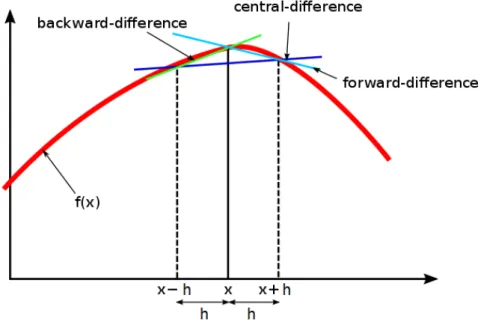
Boundary value problems are frequent in image processing which is why different finite difference methods are commonly used to approximate derivatives in order to obtain numerical solution of the differential equa-tions. One such finite difference takes the mathematical expression of f(x+b)− f(x+a). Since the method presents an approximation of a derivative, the term finite difference approximation is also often used. The relation of the methods with derivatives can be found in Ref. [24].

Depending on the applications used, three forms of finite differences are commonplace. Forward ∆h[f](x), Backward ∇h[f](x), and Central

δh[f](x) differences on an arbitrary function are displayed in the equa-tions(2.20)−(2.22), respectively [25].

Forward difference shows the difference value in the form of subtraction between a function value at a selected point and another function value at a new point with added spacingh:

∆h[f](x)

h =

f(x+h)− f(x)

h . (2.20)

Backward difference shows a value of the difference between function val-ues at a selected point and at a pointx−hinstead ofx+h:

∇_h[f](x)

h =

f(x)−f(x−h)

h . (2.21)

Finally, in Central difference, a point of interest is taken and two points are taken around it with equal spacing and then the function values at both of these points are subtracted:

δh[f](x)

h =

f(x+h)− f(x−h)

h . (2.22)

14 Mathematical&Physical concepts

Figure 2.1: Backward, Central and Forward finite differences on a function at a selected point x and a random spacing value h. Out of the three approximations, the Central difference is the most accurate [26]. Plot obtained and modified from

https://www.wikiwand.com/en/Finite difference, 16/09/2019.

2.2

Physical concepts

2.2.1

Principles of MRI and SE scan

In order to explain the type of data we acquire, we need to have a general description of the techniques and physics behind the source of images. In this project, the data is obtained from a clinical imaging modality called magnetic resonance imaging (MRI).

MRI is non-invasive imaging technology which creates a spatial map of nuclei of hydrogen atoms (mostly in water and lipids). The images can be acquired in both two-dimensional as well as three-dimensional geome-tries. The intensity of the image depends on the density of protons in a bounded spatial area [27]. Using a strong magnetic field and radiofre-quency current pulses directed to go through the object, the MRI alters the spin directions of the protons within the tissue of the object. The relaxation times, i.e. the time it takes the spins to point in their initial directions, can be obtained which will provide information about the physical properties of the tissue.

14

2.2 Physical concepts 15

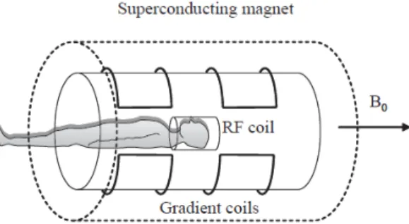
Figure 2.2: Three major parts of the MRI system. Superconducting magnet, RF transmitter and receiver, and, for simplicity, only one gradient coil.

The MRI system consists of three major parts: a superconducting mag-net, radiofrequency transmitter and receiver, and three different magnetic field gradient coils. The simplified schematic image of the system can be found in Figure 2.2. Clinical field strengths of, B0, are 1.5 and 3 T which are 60 000 and 140 000 times stronger than the earth’s magnetic field, re-spectively. Research systems at higher field strengths are coming up.

The protons, being charged particles in different types of tissue, can be thought of as small magnets as they carry spins which are an intrinsic form of describing an angular momentum, P, characterized by quantum numbers. Due to this spin, each particle also has a magnetic moment µ

which gives them magnetic properties. The magnetic momentµis directly

proportional to the magnitude of the angular momentum of the proton:

|~µ|=γ|~P|, (2.23)

whereγis gyromagnetic ratio. While being outside the magnetic field, the

magnitude of each magnetic moment is fixed. However, their orientation is completely random resulting in the net magnetization M being zero. When the protons are in the magnetic field, due to the nature of quantum mechanics, the magnetic moment can have only two quantized values. These values are the alignments at angles θ = ±54.7◦ with respect to the

direction of the B0field [27]. The positive value is termed as parallel and negative as anti-parallel which refer to the z-component of the magnetic momentµ and to the fact thatµis aligned with respect to the direction of

B0.

When the magnetic moment of the protons is aligned with respect to B0at an angle of 54.7◦, the B0field tries to align the magnetic moment with itself creating a torque, C, which is a cross product of both magnetic fields

16 Mathematical&Physical concepts

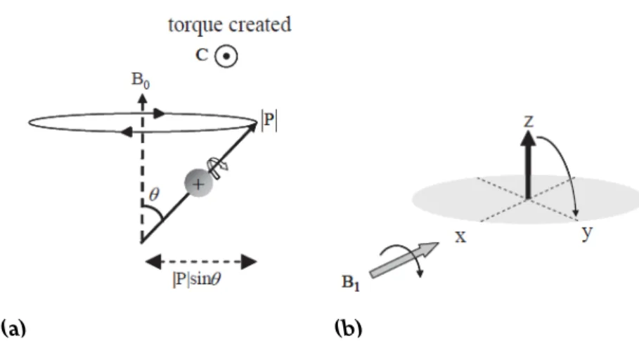
(a) (b)

Figure 2.3: (a) Precessing movement of the spins around theB0field at an angle

θ. (b) The flip of the spin direction to the xy-plane as RF pulse is applied to the

system along x-axis.

~_C=~µ×B~_{0=|µ||B0|sinθk}ˆ_{, (2.24)}

where ˆk is unit vector perpendicular to both~µ and B~0. The torque then forces the protons into the precessing movement around B0. This is due to the tangential direction of the torque with respect to magnetic moment shown in Figure 2.3a. The frequency of the precess is directly proportional to the B0field:

ω =γ|B0|. (2.25)

This frequency is called Larmor frequency,ω0. Its derivation is irrelevant for our work but can be found in Ref. [27].

While in the magnetic field, B0, all the protons are precessing in the parallel or anti-parallel directions creating a net magnetization along the z-axis parallel to the B0 field. This net magnetization is calculated by the vector sum of individual components. The magnetization only has the z-component as the components along the x- and y-axes cancel each other. The net magnetization can be rotated by applying short radiofrequency (RF) pulses perpendicular to the static field B0. The magnetic component of these pulses called B1field creates a torque that forces the net magneti-zation to rotate towards the xy-plane without affecting Larmor frequency. This process is demonstrated in Figure 2.3b. After these energy pulses are being turned on and off, an electrical signal can be detected due to Fara-day’s law of induction which states that the varying magnetic flux over

16

2.2 Physical concepts 17

time induces an electrical voltage. However, these signals do not yet con-tain any spatial information. In order to gain spatial information, the three gradient coils are, in turns, switched on to generate magnetic field gradi-ents along the three axes independently. The Larmour frequency describ-ing the precess motion of the protons depends on the magnitude of B0field and consequently on its gradients in independent directions encoding the spins spatially [27].

Before the RF pulses are applied, the system is in the equilibrium mag-netization state with a sole Mz-component. When the pulses are switched on, they create a non-equilibrium system where both Mx- and My -compo-nents are non-zero. After the pulses are switched off, the system decays back into the equilibrium which is characterized by two relaxation times: spin-lattice, T1, and spin-spin, T2, relaxations. T1 governs only the z-component of magnetization and T2 governs the x- and y-components. Relaxation times alter greatly depending on the consistency of the object which is why they can be used to classify the type of the tissue [27,28,29].

The sequence used to acquire data in this work is called Spin Echo (SE). In order to explain it, first consider only Mz-component of the net magne-tization without B1 field in the system. As the first step, an RF pulse is applied so that it flips the net magnetization to xy-plane without losing the value in comparison to the initial Mz. This pulse is termed 90 degree pulse. Due to inhomogeneities in strength of local magnetic field in the system, some spins speed up and some slow down, as the net moment precesses. This is what makes the signal decay. Another pulse, a 180 de-gree pulse, is applied to flip the spins around so that the slower ones are ahead of the main moment and faster ones are behind. At last, the fast mo-ments catch up with the main moment, while the main moment catches up with the slow ones.

Chapter

3

Theory & Methods

In this chapter, we will present, in detail, a theory of phase-based conduc-tivity mapping using data from magnetic resonance imaging (MRI) appa-ratus with Helmholtz equation and a model-based approach with regular-ization proposed by Kathleen Ropella, et al. [9]. This method will be in the centre of our work, as its main purpose and goal is to create the conductiv-ity maps using a method involving the inverse Laplacian approach which should create maps with more accuracy than with the approach that uses Helmholtz equation.

3.1

Phase-based conductivity mapping

In the highlight of the phase-based conductivity mapping is the complex permittivity which defines the electrical properties of tissue:

κ:=e−i

σ

ω

, (3.1)

where e is permittivity, σ is conductivity, and ω is the resonant angular

frequency introduced in section 2.2 as Larmor frequency. Here, the ma-terial’s ability to conduct electric current is described by the conductivity while material’s ability to resist the creation of an electric field within itself is described by permittivity.

First, by combining Faraday’s and Ampere’s laws from Maxwell equa-tions, we are able to derive the following relation between the magnetic flux density,B, and complex permittivity shown in the equation (3.1):

− ∇2B= ∇κ

κ ×[∇ ×B] +ω

2

20 Theory&Methods

where∇2_{is so-called Laplacian operator and}

µ is permeability which

de-scribes a material’s ability to support the formation of the magnetic field within itself [9].

Here, we bring out our first assumption that will contribute to inac-curacies in our conductivity map reconstructions − we assume that the complex permittivity κ is locally constant (assumption of homogeneity).

This directly results in the gradient of the complex permittivity becoming zero, and thus:

∇κ

κ ×[∇ ×B] =0, (3.3)

which, on its part, drops out the first term on the right hands side in the equation (3.2). Therefore, our now simplified equation takes the following form:

− ∇2B=ω2µκB. (3.4)

Now, we can relate the magnetic flux density to square of the complex wave number which is defined as follows [30]:

k2=µeω2−iµσω, (3.5)

which gives us the final Helmholtz equation:

∇2B+k2B=0, (3.6)

which is generally used to reduce the complexity of the analysis after the separation of variables in physical problems.

The Helmholtz equation can be rewritten with a harmonic magnetic field and it is valid for each Cartesian component so the magnetic field can be expressed as the effective magnetic field

B₁+ = (Bx+iBy) = |B₁+|eiφ

+

, (3.7)

since this transmit radiofrequency (RF) field is used in the MRI [9,30]. Here,φ+is the phase of the B+₁ field which is affected by the conductivity

of the measured object [13].

Now, we can rewrite the Helmholtz equation in (3.6) in the following form:

∇2B+₁ +k2B+₁ =0, (3.8) The core idea of using the Helmholtz equation for the phase-based con-ductivity map reconstruction is that both magnitude of the magnetic field

20

3.1 Phase-based conductivity mapping 21

and its phase are known in order to calculate the conductivity as well as permittivity of an object.

With the use of the definition of the RF field presented in the equation (3.7), we can expand the Helmholtz equation into the following form using product rule:

∇2_B+

1

|B+₁| +

2∇|B₁+|eiφ+

|B+₁|eiφ+ +

∇2_eiφ+

eiφ+ =−k

2_{. (3.9)}

From the definition of the squared complex wave number in the equa-tion (3.5), it is almost trivial to specify that conductivity is in the imagi-nary part of it and therefore solving the conductivity is done by taking the imaginary part of the expanded Helmholtz equation in (3.9) resulting in

Im

2∇|B+₁|∇eiφ+

|B+₁|eiφ+ +

∇2_eiφ+ eiφ+

=σµω, (3.10)

where the first term on the left hand side ∇2B

+

1

|B+₁| ∈ R and consequently

was dropped out. In addition to the conductivity, it might be already clear that the EPT using Helmholtz equation can also compute the permittivity

e using a similar procedure. In order to solve the expanded Helmholtz

equation (3.9) fore, the real part of the equation must be taken in the

simi-lar fashion as the imaginary part, since the permittivy can be found in the real part ofk2. However, the permittivity is not of great importance to our work and hence we will not proceed with solving the equation fore.

In the continuation with the imaginary part in the equation (3.10), the first term of the left hand side is small enough in comparison to the second term for us to approximate the equation into the following form [30]:

Im

∇2_eiφ+ eiφ+

≈σµω. (3.11)

This approximation contributes to a relatively small error in our conduc-tivity calculation, and we, therefore, choose to neglect it.

What is now left is the expansion of the numerator in order to write out the solution for the conductivity in as simple form as possible

∇2eiφ+ _=i∇(eiφ+_∇

φ+) = i(eiφ

+

∇2φ++∇eiφ

+

∇φ+)

=ieiφ+_∇2

φ+−eiφ

+

22 Theory&Methods

where we have clear distinction between real and imaginary parts which finally allows us to write the final approximation for the conductivity:

σ ≈ ∇

2

φ+

µ0ω . (3.13)

Here, the permeability was chosen to be a vacuum permeability as it is an acceptable approximation for the human body [30].

The result is the equation used for the phase-based conductivity map-ping which is extremely time efficient since the magnitude of the field is not required at all for the computation. The transmit phase data is ac-quired from the spin echo (SE) sequence. This method is valid as long as the curvature of the B₁+field is small which increases with the strength of the static magnetic field B0[13].

The main issues in the Helmholtz-based EPT as well as in the EPT in general are boundary errors and low signal-to-noise ratio (SNR). The boundary errors, as the name suggests, arise at the boundaries of scanned materials due to the assumption that the permittivity is locally constant in a material while the low SNR arises from the heavy reliance on the Lapla-cian operator highlighted in the equation (3.2). The electrical properties of the material are proportional to the Laplacian of the magnetic fields re-sulting in the amplification of all types of noise produced by the MRI scan. Multiple methods have been proposed to tackle these issues including the inverse approaches into which we will dive in the following section as we present a proposed method of inverse Laplacian to create conductivity maps more accurate than those created using the Helmholtz-based EPT method [9].

3.2

Inverse Laplacian approach

In this work, we present a model-based reconstruction approach (pre-sented by Ropella, et al. in Ref. [9]) that uses regularization in order to decrease the number of factors contributing to edge artifacts and noise amplification. In this method, inverse Laplacian,∇−2_{, is used for the} min-imization of the difference to acquired phase data from the SE scans. Apart from the transmit phase data, the method also uses information about ge-ometry of the object to confine the calculations within a certain area by introducing boundaries using support and edge masks. The method deals with 3D maps created from the collected MRI data, so all of the data will be presented as three-dimensional tensors or as in this case, we can call them three-dimensional matrices or arrays.

22

3.2 Inverse Laplacian approach 23

The proposed method to reconstruct the conductivity map using regu-larized least-squares method is as follows

σ0 =argmin

σ 1 2||

φ+

µ0ω −Lσ||

2

W1 +λW2R(σ), (3.14)

where we denote the optimal conductivity with σ0, L is the matrix

repre-sentation of the differential inverse Laplacian operator, ∇−2_{, W}

1and W2 are binary matrices used to mask out relevant areas in the reconstructed map,λis regularization parameter, and R(σ)is regularization function.

The first term is a quadratic function which is minimized resulting in enforced relationship between the acquired phase data and reconstructed conductivity map leading the reconstruction in the correct direction. This is done within the domain of the binary mask W1 which will be show-cased in the more detailed optimization analysis. The second term, is the regularizing term used to minimize the rising edge artifact and to smooth the image in the area restricted and defined by the mask W2 in the same manner as W1.

Before defining L, we need Laplacian operator,∇2, which is defined

∇2= ∂ 2

∂x2 + ∂2 ∂y2 +

∂2

∂z2, (3.15)

with, if we denote a 3D matrix as a function f(x,y,z)

∂2

∂x2f(x,y,z) =

f(x−hx,y,z)−2f(x,y,z) + f(x+hx,y,z) h2

x

, (3.16)

∂2

∂y2f(x,y,z) =

f(x,y−hy,z)−2f(x,y,z) + f(x,y+hy,z) h2

y

, (3.17)

∂2

∂z2f(x,y,z) =

f(x,y,z−hz)−2f(x,y,z) + f(x,y,z+hz) h2

z

, (3.18)

where hx,y,z are the voxel dimensions. These equations are essentially second-order central finite differences which are an approximation of the second order derivative which Laplacian operator represents in three di-mensions [25]. If in the image all the voxels are identical (isotropic unit voxels) and the origin of the matrix is at its center, the resulting matrix representation of∇2_isR3×3×3_{array with the following values}

∇2(0, 0, 0) =−6,

24 Theory&Methods

else zero. (3.19)

This is a representation when the voxel dimensions hx,y,z = 1. In other cases, these resolution parameters must be added to the values of the array elements according to equations (3.16)-(3.18).

The matrix form of the inverse Laplacian, L, is first calculated by zero-padding the kernel∇2(x,y,z) to match the dimensions of the magnitude and phase data. Next, we take its 3D fast Fourier Transform (FFT) and invert each individual component value in the resulting matrix. However, before inverting the components, a small offsetδmust be added to the zero

valued DC term in the origin of the matrix in order to avoid zero division upon the inversion of the matrix components. After the offset is added and the components are inverted, we take the inverse FFT of the resulting kernel and we obtain the final form of the matrix L.

The reason this procedure is done is the fact that the inverse transform is given by the inverse of the matrix in question as shown in equation (2.13). If we invert every element of this matrix in Fourier domain, the outcome of the inverse Fourier Transform is, then, inverse of the matrix that the Fourier Transform was initially applied to.

The matrix L can be thought of as a filter and just as explained in the section 2.1.1, the filter is applied to an image or in our case, to the map using convolution. So, essentially, the Lσ representation in the equation

(3.14) is the convolution operation between the two 3D arrays:

Lσ :=L∗σ =F−1F {L} · F {σ} . (3.20)

where ”·” denotes pointwise multiplication and therefore it is important that both L andσare of the same dimensions. Since, in the entirety of this

work, we will be dealing with 3D arrays, for the sake of simplicity, we will continue using this notation in the further calculations.

The support mask W1 is created by defining a certain threshold in the data of the magnitude of data. The values equal and above this threshold value will equal 1 while the rest will be turned to zero. This creates a binary map which will dictate the location where the reconstruction of the conductivity map will be done. The rest of the area will be neglected in the calculations due to the zero values in the mask.

The edge mask W2can be created using different edge detection meth-ods and in this work we specifically used Canny edge detection operator that uses multiple stages in its algorithm [31]. This operator is applied to the magnitude map which produces a clear image of the edges of an ob-ject. These edges are then converted to zero values and the rest to equal value 1. Lastly, it is combined with W1 mask in order to mask only the

24

3.2 Inverse Laplacian approach 25

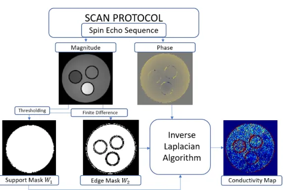
Figure 3.1:Reconstruction process from the data acquisition to conductivity map reconstruction. Phase and magnitude data are acquired from SE sequence. Masks

W1 andW2 are obtained from geometry data and subsequently combined with

phase data in IL algorithm to construct a conductivity map of the object.

object area excluding the edges within the object. The resulting mask dic-tates where the regularization will be applied. Examples of both W1and W2masks are shown in Figure 3.1.

The regularization function,R(σ), consists of a squared Euclidian norm

of potential functionΨ(Cσ)where C is the first order finite difference

oper-ator in the matrix form which gives out smoother conductivity map. When the regularization function is multiplied with W2, it calculates a weighted sum of the differences between a voxel and its adjacent neighbour in every direction.

The optimal conductivity, σ0 in equation (3.14) is solved with the use

of nonlinear conjugate gradient method (NCGM) [32,33,34]. This method generalizes the conjugate gradient method which solves unconstrained optimization problems such as ours with an iterative algorithm [33,34].

26 Theory&Methods

3.2.1

Approach without regularization

If the regularization is not included in the reconstruction of the conductiv-ity map, the problem reduces to

f(σ) = 1

2||

φ+

µ0ω −Lσ||

2

W1. (3.21)

Since NCGM is a gradient-based method, the main idea of it is to find a local minimum of a nonlinear function using its gradient,∇σf, which in-dicates the direction of the maximum ascent. In order to show the opposite

−maximum descent (or the steepest descent), simply the negative of the gradient,−∇σf, is taken. The form of solving the iterative optimization problem is as follows:

σn+1=σn +αndn, (3.22)

where αn is a step size which varies at each step of the iterationn and is obtained by a line search, anddn is the search direction defined as

dn = (

−∇σf, for n =0;

−∇σf +βndn−1, for n ≥1,

(3.23)

where βn is a direction parameter (not to be confused with regularization parameter).

The algorithm itself can be broken down into five general steps: 1) Calculation of the steepest descent:∆σn =−∇σf(σn),

2) Computation ofβnwith one of the two methods shown below:

βFRn = ∆σ T n∆σn

∆σ_nT₋₁∆σn−1,

βPRn = ∆σ T

n(∆σn−∆σn−1)

∆σ_nT₋₁∆σn−1 ,

3) Update of the conjugate direction: dn =∆σn+βndn−1, 4) A line search: Optimization ofαn :=argmin_σ f(σn+αdn),

5) Update of the map: σn+1=σn +αndn,

whereβ0is set to zero, so that the result is correct forn =0 in the equation (3.23), andσ0is an initial educated guess of the conductivity map.

The two formulas in the second step of the algorithm are named after Fletcher-Reeves and Polak-Ribiere methods, respectively [33,35]. Both of these formulas help the algorithm achieve the same result. However, the speed or the number of steps at which the algorithm converges may vary for these methods. In addition to the two methods presented, there are

26

3.2 Inverse Laplacian approach 27

other methods [33]. Regardless, in this work, we focus on and utilize only the two presented methods.

Some steps, namely the first and the fourth steps require more par-ticular look into the more detailed way of computing the gradient and performing a line search, respectively.

First, the algorithm requires the gradient of our function, ∇σf(σn), which is the essential part of the minimization. Its calculation is fairly simple when the 3D arrays in the function are vectorized. We first expand the function, f(σ), in the following way

f(σn) = 1 2

|| φ

+

µ0ω||

2 W1 −

φ

+

µ0ω, Lσn

W1−

Lσn, φ

+

µ0ω

W1+||Lσn||

2 W1

,

(3.24) where due to the fact thatφ+, L, and σare real, we are allowed to exploit

the commutative property

φ

+

µ0ω, Lσn

=

Lσn, φ

+

µ0ω

, (3.25)

which allows writing the function as

f(σ) = 1

2

|| φ

+

µ0ω||

2 W1−2

Lσn, φ

+

µ0ω

W1+||Lσn||

2 W1

. (3.26)

Now, we can take the gradient of this function resulting in

∇σf(σn) = 1 2 −2 L, φ +

µ0ω

W1+

L, Lσn_W

1 +

Lσn, L_W

1

:=LLσn− φ

+

µ0ω

W1

, (3.27)

where we used the property identical to the one in equation (3.25) and the final notation with reshaped matrices was written with the accordance to the rules we previously set. The reason we were able to rewrite it in the final form was due to the fact that three-dimensional maps are convoluted with the inverse Laplacian, L, which is a self-adjoint matrix. A detailed view on derivation of the gradient of the 2-norm of vector residual can be found in Appendix A.

In order to perform a line search, we need to optimize step size α in

accordance to the fourth step of the algorithm. To obtain the solution for

αn, we have to solve

28 Theory&Methods

Here, we use inner product also known as dot product notation which is more optimal for solving scalars. First, we expand the function as:

f(σn+αndn) = 1 2||

φ+

µ0ω −Lσn−Lαndn||

2 W1 =

1

2||rn−Lαndn|| 2

W1, (3.29)

where rn = φ+

µ0ω −Lσn denotes the residual between the phase map ac-quired from MRI and phase map calculated using convolution between inverse Laplacian and conductivity map of iteration step n, and αn is a scalar. Further expansion takes form

f(σn+αndn) = 1 2

||rn||2_W

1−

rn,αnLdn_W

1−

αnLdn,rn_W

1+α

2

n||Ldn||2W1

.

(3.30) Since we are optimizingαn which is a scalar, we are allowed to vector-ize both rn and Ldn and they both are real valued (L,φ+,σn,dn ∈ R). In addition, L is a self-adjoint matrix giving us the following commutative relation:

αnrn, Ldn) =αnLdn,rn. (3.31) Using the property in equation (3.31), we are finally able to write the function in (3.30) in the following form

f(σn+αndn) = 1 2

||rn||2−2αnLrn,dn+α2_n||Ldn||2

W1

, (3.32)

where it is good to note that Lrn is the gradient required for computation of the direction for the steepest descent in the first step of the algorithm. Next, we take the derivative of the function with respect toα

∂αf(σn+αndn) =−

Lrn,dn

W1+αn||Ldn||

2

W1, (3.33)

which allows us to obtain the final formula for the optimizedα

αn =

Lrn,dn

W1

||Ldn||2 W1

, (3.34)

where, dot product between Lrn anddn, and squared norm of Ldnare kept within the domain of support mask W1.

As the final remark, we note that in order to keep the calculations and reconstruction within the desired domain, we must apply the sup-port mask W1 to the algorithm of the NCGM as previously stated. To do

28

3.2 Inverse Laplacian approach 29

so, we apply the mask to the initial form of the conductivityσ0in equation (3.22) using pointwise multiplication. In next steps of the iteration process, we apply the mask only to the gradient of the entire function in the similar fashion. Since the outcome of every step of the algorithm depends on the gradient, the effect of the application of the mask will automatically trans-fer to the outcomes of these steps as shown in derivations above. Hence the mask is applied only once which significantly reduces the computation complexity of the algorithm.

3.2.2

Approach with regularization

Upon having the regularization term in equation (3.14), adding the reg-ularization to the algorithm is not as difficult of a task as might seem at first. The only parts of the algorithm that need to be modified are the first and the fourth steps which were inspected closely in the previous section. The regularizing term is added to the data term, minimum of which the algorithm strives to find. This means that we do not need to perform the calculations for the gradient and the step size from the very beginning. Instead, we can take readily calculated parts from the data term in the previous section and add differentiated terms to it.

Before presenting formulas for the gradient of the function and the step size, we define the regularization function

R(σ) = ||Aσ||2_W2, (3.35)

where the use of such regularization function is called Tikhonov’s regu-larization. The first finite difference operator, A, is picked to be suitable regularization matrix [34]. This way, values of the regularization function grow in the manner of a quadratic function which allows to penalize the roughness in the conductivity map in nonlinear fashion [9]. Depending on the data and the object we are dealing with, occasionally Laplacian (sec-ond order finite difference) can also be used as the regularization matrix. However, it is of great rarity that Laplacian produces better results than the first order finite difference operators [36].

Matrix form of the first finite difference operator, A, is constructed the same way as the Laplacian operator in the previous section. Only this time, we follow the rules of operators introduced in Chapter 2 in equations (2.20)-(2.22). The three finite difference operators take the following matrix forms:

Central finite difference:

30 Theory&Methods

else zero, (3.36)

Forward finite difference:

F(0, 0, 0) =−3

F(1, 0, 0) =F(0, 1, 0) =F(0, 0, 1) = 1,

else zero, (3.37)

Backward finite difference:

B(0, 0, 0) =3

B(−1, 0, 0) = B(0,−1, 0) =B(0, 0,−1) =−1,

else zero. (3.38)

Essentially, we use these matrices as any other operator in this work by convoluting them together with our 3D maps representation of which is shown in equation (3.20). However, these finite difference operators are not self-adjoint matrices forcing us to define their adjoints separately in our calculations.

Now, we compute the gradient of the function with the regularization. We take the calculated gradient from the equation (3.27) and add the gra-dient of the regularization term to it

∇σf(σn) = L _φ+

µ0ω −Lσn

W1

+λ∇σ ||Aσn||2W2

=L φ

+

µ0ω −Lσn

W1

+λW2adj(A) Aσn

, (3.39)

where adj(A) is adjoint of A which in three dimensional case does not equal the transpose of A unlike in two-dimensional case.

Computing the step size can be done in the similar manner by taking already existing calculations from the equation (3.32), adding the regular-ization term to it, and expanding it

f(σn +αndn) = 1 2

||rn||2−2αnLrn,dn+α2n||Ldn||2

W1

+λ||A σn +αndn||2_W2

= 1 2

||rn||2_W

1 −2αn

Lrn,dn_W

1+α

2

n||Ldn||2W1

30

3.2 Inverse Laplacian approach 31

+λ

||Aσn||2_W2 +αnAσn, Adn_W

2+αn

Adn, Aσn_W

2 +α

2

n||Adn||2W2

, (3.40) wherern = φ+

µ0ω −Lσn is the residual. Next, we take the derivative of the function with respect toα

∂αf(σn+αndn) = −

Lrn,dn

W1 +αn||Ldn||

2 W1

+λ

Aσn, Adn_W

2 +

Adn, Aσn_W

2 +2αn||Adn||

2 W2

. (3.41)

Unlike in the case with Laplacian, the finite difference operator is not self-adjoint,

Aσn, Adn 6=Adn, Aσn, (3.42) and therefore equation (3.41) remains unchanged. The final stage of opti-mization is done by solving step size,α, from∂αf(σn +αndn) = 0

αn =

Lrn,dn

W1−λ

Aσn, Adn_W

2 +

Adn, Aσn_W

2

||Ldn||2

W1+2λ||Adn||

2 W2

. (3.43)

Chapter

4

Results & Discussion

In this chapter, we will present our results of conductivity map reconstruc-tions introduced and discussed in Chapter 3. Apart from demonstrating the reconstruction for both cases: without and with regularization, respec-tively, we will show different ways of determining parameters needed in the algorithm along with functionality and practicalities of the algorithm itself. We perform first analysis on simulated data where real conductivity of an object is known in order to estimate the accuracy of the reconstructed conductivity values before moving onto experimental data.

4.1

Approach without regularization

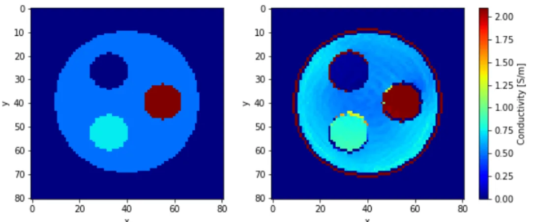
The conductivity map of the simulated object can be found on the left hand side of Figure 4.1 and the map on the right side displays the outcome of the time efficient Helmholtz-based conductivity reconstruction of equa-tion (3.13) where we convolute Laplacian with acquired phase data. We show central slices of the reconstructed maps in order to demonstrate the results in two dimensions.

34 Results&Discussion

Figure 4.1:Conductivity maps for the simulated data. First image is real conduc-tivity of the simulated object and the second is reconstruction using Helmholtz-based EPT. X and Y -axes indicate number of pixels in proprietary direction. Colour scale indicates the intensity of the conductivity values in siemens per me-ter.

theorem introduced in section 2.1.3 where the Fourier series on piecewice differentiable function starts behaving peculiarly as it sums overshoot at sharp transitions in values. The series has high oscillations at the sharp edges which do not die out when more terms are added to the overshoot and hence we see the boundary artifacts [37]. The ringing within the in-ner tubes remains due to the fact that the number of added terms is finite and therefore the values between higher edge transitions remain oscilla-tory. We will observe the SNR later on in this chapter as initially we did not add noise to the phase data used for the reconstruction.

We start our reconstructions with initial phase data from the simula-tion without the regularizasimula-tion term. We kept the data noise free in order to observe possible benefits of the inverse Laplacian approach for the com-parison to the direct Helmholtz approach before diving into the smoothing abilities of the regularizer.

As the first step, in order to determine useful offsetδfor the DC

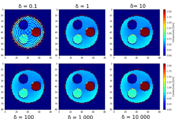
coeffi-cient of the inverse Laplacian to avoid the division by zero, we tested the algorithm with a range of offset valuesδ = [10−1, 104]. The results with

different offset values are displayed in Figure 4.2 for a certain number of iterations with each value. Forδ =10−1, the conductivity map is severely

underdeveloped displaying large fluctuations in form of rings in values across the entire domain of W1 mask with high values spread out across and beyond the boundary artifacts. Forδ = 100 and δ = 101, noticeable

cross hatching is present close to the edges of W1 mask domain. Offset

34

4.1 Approach without regularization 35

Figure 4.2: Conductivity maps reconstructed using the inverse Laplacian ap-proach with different δ offset values added to the DC coefficient without

regu-larization. δwas varied between values10−1 and104. Every reconstruction was

run over the same number of iteration steps.

δ =102seems to have the closest values to those of the map reconstructed

using the Helmholtz EPT equation while δ = 103 and δ = 104 have

in-crease in the conductivity values close to the edges of the outer tube. We, henceforth, conclude that the most reliable offset value is aroundδ = 100

and continue performing further experiments using this value.

Throughout our experiments, we noticed that δvalue is dependent on

the size of the object as well as the dimensions of the voxels i.e. the resolu-tion of the image. Therefore, it should be possible to determine a suitable offset value using these parameters. However, as of the moment this work is written, we have not focused on determining the optimalδvalue by any

other than experimental means.

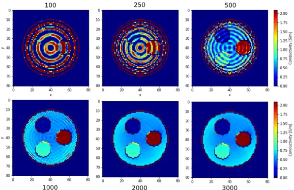
In Figure 4.3, we display the progress of the reconstruction using the offset valueδ = 102at different number iterations until the minimization

36 Results&Discussion

Figure 4.3: Reconstruction of the conductivity map with the initial guess of a map with nothing but zero values withδ = 102used for the inverse Laplacian.

The observations were made after 100, 250, 500, 1000, 2000 and 3000 iterations. In this case, the number of iteration needed before the reconstruction converged was approximately 3000.

with the number of iterations, the sharp edges between the rings start de-creasing and finally converge to nearly identical values. However, when the minimization converges, some ringing is still present due to the fact that the added terms do not kill the overshoot produced by the Fourier series as described by the Gibbs phenomenon [37].

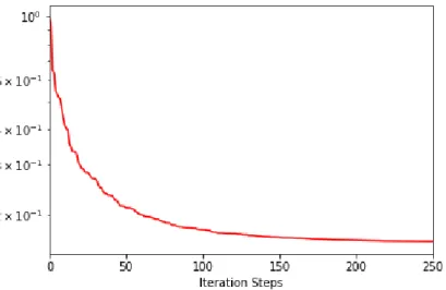
In Figure 4.4, we display a normalized cost function which is represen-tation of functional convergence as a function of number of iteration steps during this reconstruction. The functional is simply a squared Euclidian norm of the residual between initial phase data and reconstructed phase map by applying inverse Laplacian to conductivity map within the W1 domain:

F(σ) =|| φ

+

µ0ω −Lσ||

2

W1 (4.1)

We see a huge drop within 250 iterations which makes sense since the re-constructions started from a zero-valued conductivity map. Past the point of 250 iterations, the algorithm mainly works on equalising the difference

36

4.1 Approach without regularization 37

Figure 4.4:Normalized cost function of the reconstruction for 250 iteration steps. Here the functional values are displayed as a function of number of iteration steps.

Figure 4.5: Step sizes as a function of number of iteration steps. Step size con-verges to nearly zero for the large number of iteration steps.

between the rings resulting in a smaller drop of the cost function. This highlights the fact that the sequence is monotonic [38]:

38 Results&Discussion

Figure 4.6: Comparison between conductivity maps reconstructed using Helmholtz EPT and inverse Laplacian approach with added noise making SNR=

100. (a) Helmholtz EPT (b) Inverse Laplacian approach.

of iteration steps which indicates that we are moving steadily towards the local minimum of the functional. Since in our case we have a quadratic function, it has only one minimum which is the global minimum of the minimization problem. The step size as a function of iteration steps in Figure 4.5 further confirms the convergence as it reduces to nearly zero for a large number of iterations.

As the final analysis for the reconstruction without the regularization applied to the conductivity, we add the noise to the initial phase data of the simulation and compare the differences between SNR for both the Helmholtz EPT and the inverse Laplacian approach. The noise we add is additive white Gaussian noise (AWGN) to the imaginary part of the field magnitude with mean value set to 10−8and standard deviation set to 10−10 making SNR=100. The results are displayed in Figure 4.6.

The difference between the two methods of reconstruction are nearly identical with some exceptions in form of higher noise values close to the edge of the tubes in the inverse approach. The reconstruction using the unregularized inverse Laplacian approach does not get rid of the noise at all and reconstructs the image preserving nearly identical SNR to the one in Helmholtz EPT. Occasional local noise that is higher in the Inverse Laplacian approach could possibly correspond to the fact that noise can be amplified even further due to the added terms with amplified noise in the Fourier series in the reconstruction.

With these arguments, we conclude that the conductivity

reconstruc-38

4.2 Approach with regularization 39

tions obtained using the unregularized inverse Laplacian based method correspond to the those obtained via conventional deconvolution using the Laplacian kernel. This is in line with the mathematical formulation, as no additional constraints or a priori information has been incorporated. In addition, the unregularized method is more time consuming than the conventional method.

4.2

Approach with regularization

4.2.1

Simulated data

In this section, we use the same method of reconstruction as in the pre-vious section, except now we add the regularization term into our func-tional:

F(σ) = || φ

+

µ0ω −Lσ||

2

W1 +λ||Aσ||

2

W2. (4.3)

We first look at the results in this approach using four different finite dif-ference operators A − Laplacian i.e. second order finite difference, and first order Forward, Backward, and Central finite difference operators. We add complex white Gaussian noise to the input data making SNR= 100 and compare the results among each other and to the Helmholtz EPT re-construction. We show the difference between the reconstruction using only the support mask W1defining the object domain, and using both the support mask W1, and the edge mask W2which delimits inner tubes from the general domain. Finally, we compare the approach with regulariza-tion to Helmholtz EPT with applied Gaussian filter to determine whether the inverse approach with regularization has any advantages over the Helmholtz EPT.

In order to reconstruct the conductivity map with regularization penalty from any desired initial guess, a right regularization parameterλmust be

selected. It determines the balance between the term that models accu-rate data and the smoothing regularization term. While, different ways of choosing an optimal value for λ exist [9], we setλ = 0.1 and performed

regularization on the initial guess corresponding to the outcome of the Helmholtz EPT.

40 Results&Discussion

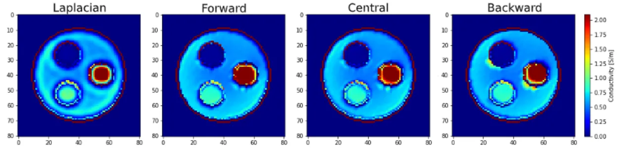
Figure 4.7: Conductivity reconstruction using Laplacian operator and Forward, Central, and Backward finite difference operators in the inverse Laplacian ap-proach with regularization on data with SNR=100.

Adjoint matrix to Forward finite difference:

adj(F)(0, 0, 0) =−3

adj(F)(−1, 0, 0) =adj(F)(0,−1, 0) = adj(F)(0, 0,−1) =1,

else zero, (4.4)

Adjoint matrix to Backward finite difference:

adj(B)(0, 0, 0) =3

adj(B)(1, 0, 0) = adj(B)(0, 1, 0) =adj(B)(0, 0, 1) = −1,

else zero. (4.5)

However, as the adjoint operator to Central finite difference operator turned out not to be trivial to obtain, we used forward differencing at ev-ery odd iteration step and backward differencing at evev-ery even number of steps. This should, in principle, operate in the same fashion as the central differencing. This can be seen from a sum of forward and backward dif-ferences in equations (2.21)-(2.22) resulting in central difference. Hence, we will keep referring to this operation as central differencing. The Lapla-cian is a self-adjoint matrix so it does not require separate specification concerning the adjoint matrix.

Results of the conductivity maps using the four operators in the larizer can be found in Figure 4.7. Using the Laplacian operator as regu-larization matrix somewhat smooths the map equally in every direction. However, it produces severe ringing effect in areas close to the edges set by the edge mask W2and does not seem to be able to equalize them. This

40

4.2 Approach with regularization 41

Figure 4.8:The effects of the regularization using Central finite difference opera-tor with application of different masks. (1) Reconstruction without regularization with SNR=100(2)W1mask (3)W2mask (a) Regularization with onlyW1mask

(b) regularization with bothW1andW2masks.

is due to the second order derivative approximation that Laplacian repre-sents which, in general, is less accurate than first order derivative approx-imation that the rest of the operators correspond to. The rest of the opera-tors indeed do not produce such a severe ringing effect at the boundaries of the edge mask and instead improve the overall uniformity of the re-constructed conductivity. We see that the main areas within the tubes are smoothened nicely excluding small areas at the boundaries of the inner cylinders. Forward difference produces the smoothing in one direction which is the lower left corner of the map. Backward difference operates in the similar fashion with the only difference being the inclination into the opposite direction. These effects result in small imbalance within the tubes with the edges in the direction of the operators obtaining conductivity val-ues with more accuracy than the edges on the opposite sides. On its part, the central difference operates as a middle ground between forward and backward operators. It smoothens areas evenly without emphasis in one of the directions and produces slight inaccuracies along the sharp transi-tion edges in values.

42 Results&Discussion

Figure 4.9: Comparison between Gaussian filter and smoothing using inverse Laplacian approach with regularization with Central finite difference operator. Error maps between reconstructed conductivity and real conductivity are dis-played below. These maps confirm that the inverse approach with regularization reconstructs maps with higher accuracy than Helmholtz EPT.

shift in the accuracy is directed into the desired location.

In order to showcase the importance of the edge mask in the regular-ization, we show the effect of the smoothing solely by using threshold mask W1and by applying both W1and W2masks. We choose Central fi-nite difference operator for this comparison. The comparison is displayed in Figure 4.8.

As one can see, without the use of the edge mask W2 that would set boundaries at the edges of the tubes, the difference is also taken with val-ues outside the object resulting in the wrong valval-ues washing into the do-main of the object as well as the inner tubes. This is precisely what the edge mask was designed to prevent. We can see when the mask is ap-plied to the regularization, it preserves the conductivity values near the edges by preventing the differential operation from applying on the sharp transitions in conductivity values.

42

4.2 Approach with regularization 43

Figure 4.10: Comparison between direct Helmholtz EPT conductivity map re-construction and inverse Laplacian approach with data with three different SNR levels.

Finally, we compare the results from the penalized regularization us-ing Central difference operator to smoothened outcome of the Helmholtz EPT with Gaussian filter with standard deviation set to one [39]. In addi-tion, we demonstrate the amount of difference between the reconstruction and the real conductivity displayed in the beginning of the chapter. The comparison is found in Figure 4.9.

We observe that Gaussian filter smooths the conductivity values more evenly in the areas where conductivity values are supposed to be constant. However, these values are higher in the comparison to the real con-ductivity and additionally it creates enormous voids and overshoots at the sharp transition jumps resulting in more inaccuracies than the regu-larization especially since these voids in parts overlap with the inner tube hence removing parts of possibly desired object.

44 Results&Discussion

steps are required which take notable amount of time [40]. For this reason alone, the MRI acquisition time increases significantly in order to increase the SNR. By applying the inverse Laplacian approach to the data with rel-atively low SNR, the acquisition time from MRI and reconstruction time of more accurate conductivity maps are reduced. This is due to the fact that if the initial guess in the inverse approach is a map from Helmholtz EPT, the algorithm reaches the convergence point within 100 iterations which takes 1−30 seconds depending on the size of the input data and the resolution of reasonably sized objects.

To further confirm these observations, we compare the results between the outcome of the Helmholtz EPT and the inverse approach with regu-larization on the same data with three levels of SNR: 1, 50, and 100. The comparison is found in Figure 4.10.

In the future, an optimal method to choose the correct regularization parameter λ could be implemented which would allow the

reconstruc-tion of the maps with regularizareconstruc-tion from any arbitrary initial guess. On average, throughout this work, the reconstructions with arbitrary initial guesses reached the point of convergence within 5−10 minutes, again, depending on the size of the input phase data and image resolution. This shows that more accurate maps can be acquired faster with regularized inverse approach than using the additional MRI scans.

4.2.2

Phantom data

In addition to simulated data, we also run the algorithm on data from two different scans on the same phantom. Table 4.1 provides important characteristics of the phantom made and extracted from Ref. [41]. For us, the most important information are the variations in conductivity between the tubes which are measured to be between 0.11−2.24 S/m.

Table 4.1: Recipes used for the fabrication of the cylindrical phantom extracted from Ref. [41]. Important information for our experiments is contained within the measured conductivity data.

44

4.2 Approach with regularization 45

Figure 4.11: Results of the conductivity map reconstructions using Helmholtz EPT and Inverse Laplacian approach with data from two different phantom scans. Scan 1 is multi-slice turbo spin-echo scan and Scan 2 is balanced steady state free precession scan.

The first scan was multi-slice turbo spin-echo scan (MSTSE) while the second was balanced steady state free precession scan (BSSFP).

Figure 4.11 shows a comparison of the results between Helmholtz EPT and the inverse approach with regularization with the data from the two scans. We first display the images of the MRI signal magnitude to show the geometry of the phantom and the location of the inner tubes. In ad-dition, we see the magnitude of the signal which, in principle, should be proportional to the conductivity of the object.

We see that the Helmholtz EPT produces extremely noisy and unre-solvable conductivity maps where only the geometries of the phantom can be resolved. On the contrary, we see that the inverse Laplacian ap-proach produces smoothened images, confining the different conductivity values within defined regions of the edge mask W2, proving its functional-ity. Interestingly, we see clear variations between the desired conductivity values in the outcomes of both scans although the outcome of the data from the second scan is more evenly smoothened. As a down side, we see that in the second scan, the conductivity values do obtain significant errors close to the edges of the tubes.

46 Results&Discussion

Figure 4.12:Comparison of reconstructed conductivity maps using different edge masks.

how the edge mask is defined. Comparison of the conductivity reconstruc-tion with two different edge masks is displayed in Figure 4.12.

We see that when the edges of the inner tubes of the edge mask are more robustly defined, the correct conductivity values spread out more evenly across the confined areas of the tubes. However, as a trade off, we observe a rising boundary artifact at the bottom of the map. As of the moment of this thesis, we are not certain what causes this artifact to emerge.

Although we present only the center slices of our obtained maps, the conductivity values do not vary significantly as we inspect other slices while moving away from the center.

These observations confirm that the algorithm of regularized inverse Laplacian approach also works on acquired MRI data with phantoms. In addition, it produces conductivity maps which are more accurate and ro-bust than those of the Helmholtz EPT. However, dependence of the ac-curacy of the conductivity on the edge mask was observed which may require further inspection in the future.

46