Genome-wide Analysis of Transcriptional Regulation in the Murine Liver
Daniel M. Gatti
A dissertation submitted to the faculty of the University of North Carolina at Chapel Hill in partial fulfillment of the requirements for the degree of Doctor of Philosophy in the
Department of Environmental Sciences and Engineering, Gillings School of Global Public Health
Chapel Hill 2010
Approved by:
Ivan Rusyn, M.D. Ph.D.
David W. Threadgill, Ph.D.
Fred A. Wright, Ph.D.
Rebecca Fry, Ph.D.
ii Abstract
Daniel M. Gatti
Genome-wide Analysis of Transcriptional Regulation in the Murine Liver
(Under the direction of Ivan Rusyn, M.D. Ph.D.)
iii
iv
Acknowledgements
v
Table of Contents
List of Tables………... vi
List of Figures ……… vii
List of Abbreviations ……….……. ix
Chapter I. Introduction………..….……. 1
II. FastMap: Fast eQTL Mapping in Homozygous Populations ………. 10
III. Genome-level analysis of genetic regulation of liver gene expression networks ………...………..……. 37
IV. Sex-specific Gene Expression in the BXD Mouse Liver …………..……. 69
V. Replication and Narrowing of Gene Expression Quantitative Trait Loci in Inbred Mice ………..……….…………... 103
VI. MicroRNA Expression Profiling of the Mouse Liver ……….. 128
VII. Conclusions and Future Directions ………... 149
VIII. References ……..……….………... 158
vi List of Tables
Table
2.1. FastMap eQTL Mapping Times ………..………. 26 2.2. FastMap tree construction and association mapping times with increasing
vii List of Figures
Figure
2.1. The Subset Summation Tree ………..………….. 15 2.2. FastMap application GUI ………..……….…….. 22 2.3. FastMap scales linearly with increasing numbers of genes and SNPs .……... 27 2.4. SNP Similarity matrix demonstrates population stratification among
laboratory inbred strains ………..………..…… 30 2.5. Strata median correction dramatically improves transcriptome map ……….. 33 2.6. FastMap eQTL mapping results almost equivalent to those obtained with
R/qtl ……….………... 34 3.1. WebQTL interval mapping reveals genetic control of gene expression …….. 49 3.2.Genome-wide clustering of the genetic control of gene expression in liver
……..…….………...………... 52 3.3. Tissue-specific transcriptome maps reveal differences and similarities in
genetic regulation of gene expression ……….……... 56 3.4. Chr12 locus is a master-regulator of gene expression in mouse liver ………. 58 3.5. In silico discovery of gene expression to phenotype correlations using
WebQTL ………. 64 3.6. WebQTL-assisted strain selection for phenotypic profiling ………... 67 4.1. Comparison of expression of 20,868 genes in livers of male and female
BXD recombinant inbred mice ………..………. 75 4.2. KEGG and Gene Ontology categories which exhibit most significant sex
bias in mouse liver gene expression ……… 80 4.3. Sex-specific transcriptome maps reveal differences and similarities in the
viii
4.5. Differential correlation of gene expression occurs between males and
females, independent of expression level differences ………..……….. 88 4.6. Correlation analysis of gene expression reveals sex-specific clusters …... 92 5.1. Transcriptome maps from BXD and MDP ………... 112 5.2 Reduction in eQTL hotspot width using laboratory inbred strains………….. 118 5.3. Haplotype analysis of Chr 12 eQTL hotspot. ……….…... 120 5.4 eQTL replication cannot occur in IBD regions ………
….
122 6.1. Liver miRNA expression is consistent across genotype ………...……. 133 6.2. Expression of the top 95% of miRNAs detected in the mouse liver in this study compared with other studies ……… 135 6.3. MiRNA expression correlation is consistent between the MDP and BXD strains ………... 136 6.4. MiRNAs that are closely located in the genome are more likely to bepositively correlated ……….………. 137 6.5. P-value distributions from the correlation of a miRNA with all transcripts on
the array ………... 138 6.6. MiRNA expression is not correlated with the expression of host
ix List of Abbreviations
BXD: Recombinant Inbred cross derived from C57BL/6J and DBA/2J.
eQTL: gene Expression Quantitative Trait Locus (Loci)
MDP: Mouse Diversity Panel
QTL: Quantitative Trait Locus (Loci)
Chapter 1
Introduction
2
In vivo toxicity screens and mechanistic studies are often carried out in a single strain of mouse (Rao et al. 1998; Morgan et al. 1999; Constan et al. 2002). This is done in order to fix as many variables as possible and has the benefit of standardizing the genotype across multiple chemicals. While this approach provides mechanistic information about toxicant activity in a single genetic background, the reality of human toxicity is more complex, including both diverse genetic backgrounds and uncontrolled environmental effects. Environmental interactions such as synergistic or additive effect of multiple toxicants, nutritional and disease status are important aspects of human toxicology. Genetic background is also an important component of toxicity responses (Chorley et al. 2008; Lowes and Buttrick 2008). A successful in vivo approach to modeling the effects of genetic diversity on toxicity will both improve the prediction of toxicity in humans as well as improve the identification sensitive sub-populations.
3
When research into the genetic basis of toxicity is initiated, the responsible genes could lie anywhere in the genome. A forward genetics approach, in which the genetic basis of this toxicity investigated, is a reasonable approach to this problem. The first step is to search for evidence that the responsible genes lie in certain chromosomal regions by searching for correlation between the toxicity phenotype and genotype at loci throughout the genome. This is often carried out using quantitative trait locus (QTL) mapping (Lander and Botstein 1989; Haley and Knott 1992). This involves selecting or breeding a genetically segregating population, such as a backcross or intercross of two inbred parental strains, which demonstrates quantitative variation in the toxicity phenotype of interest. This quantitative phenotype, such as liver histology score or serum alkaline aminotransferase levels, is measured in each individual, who is then genotyped at a number of markers across the genome. A statistic of association, such as a likelihood ratio statistic or a linear model, is then calculated between the phenotypic values and each marker. QTL mapping of clinical phenotypes has been used to study ethanol related behavior (Crabbe 2002), ethanol metabolism (Grisel et al. 2002), iron transport (Wang et al. 2007) and other diseases and phenotypes.
4
by searching for eQTL that are co-located with clinical trait QTL, thus implicating the gene(s) with eQTL at the same locus as influencing the clinical trait (Schadt et al. 2003). This type of analysis pre-supposes that some traits are influenced by expression variation alone as opposed to non-synonymous coding SNPs, but data from natural populations suggests that this is not an unreasonable assumption (Oleksiak et al. 2002).
5
The accuracy of cis-eQTL detection has been called into question due to the possibility of SNPs residing within the sequence queried by microarray probes (Doss et al. 2005; Alberts et al. 2007; Ciobanu et al. 2010). Microarray probes are designed based on the reference sequence of C57BL/6J. Transcripts in other strains with polymorphisms in the probe sequence will bind with lower affinity than the C57BL/6J transcript, giving the false appearance of allele specific expression levels associated with the transcript location, which is the defining characteristic of a cis-eQTL. Studies in which shorter 25 nucleotide microarray probes are used (Alberts et al. 2007) appear to be more significantly affected than studies that use longer 50 to 60 nucleotide long probes (Doss et al. 2005; Ciobanu et al. 2010). This is consistent with the hypothesis that a SNP within a probe sequence will affect short probe more strongly than longer probes.
The validity of eQTL hotspots has also been questioned (de Koning and Haley 2005; Breitling et al. 2008) due to the possibility that sets of highly correlated genes will naturally cluster over the same genomic marker. Further, sets of highly correlated genes are likely to be part of the same Gene Ontology (GO) category and so when GO category enrichment is conducted on eQTL hotspots, they are likely to (falsely) appear biologically coherent. A permutation strategy, in which the sample labels are permuted and the expression labels are held fixed, has been suggested to address this problem (Churchill and Doerge 2008; Breitling et al. 2008). False eQTL hotspots may also arise due to intersample correlation and a mixed-model approach has been shown to eliminate spurious eQTL hotspots in mouse data (Kang et al. 2008a).
6
eQTL study; multiple testing across correlated SNPs and across multiple correlated transcripts. Multiple testing across SNPs may be addressed by permuting the sample labels in the genotype data while holding the expression data fixed (Churchill and Doerge 2008). Multiple testing across genes may be addressed using approaches based on the false discovery rate (Storey and Tibshirani 2003).
While the study of individual genes is informative and can improve our understanding of the causes of differential toxicity in populations, a broader approach that focuses on gene networks and biological pathways may produce more interpretable results. eQTL mapping can be used to generate hypotheses regarding transcriptional regulation and can be integrated with gene co-expression data to discover gene networks or pathways that are associated with a clinical trait. For example, transcript expression data in the livers of a panel of C57BL/6J x DBA/2J F2 mice was combined with obesity data and eQTL mapping to produce causal gene expression networks (Zhu et al. 2004; Drake et al. 2005). eQTL data may also be combined with estimates of transcription factor activity to infer causal relationships between transcription factors and clusters of eQTL genes (Sun et al. 2007). Other methods to infer causality between regulatory candidate genes under eQTL hotspots and the trans-regulated genes that map to the eQTL locus have also been proposed to assist in narrowing the list of candidate genes for further biological investigation (Doss et al. 2005; Peng et al. 2007).
7
(Wellcome Trust Case Control Consortium 2007). Separate work that examined liver gene expression in a smaller cohort of human samples with and without Type I diabetes found that ERBB3 did not have a cis-eQTL but that a flanking gene, RPS26, did. Since the disease phenotype and RPS26 both had QTLs in the same location, this suggested the RPS26 was a stronger candidate than ERBB3. The authors then used mouse liver and adipose expression data from several mouse crosses to construct causal expression networks for the ERBB3 and RPS26 orthologs in the mouse. They then showed that ERBB3 is not associated with any known Type I diabetes genes whereas RPS26 is associated a network of several genes that are part of the KEGG Type I diabetes pathway (Schadt et al. 2008). This type of analysis demonstrates the power of combining human and mouse data with a network based approach that has been proposed for use in drug discovery (Schadt et al. 2009) and may prove useful in toxicology.
Specific Aim 1, Fast eQTL Mapping in Homozygous Populations, consists of a hypothesis driven approach to software development in which we surmised that the conventional gene expression quantitative trait locus (QTL) mapping algorithms suffered from a lack of computational efficiency and could be greatly improved through the use of algebraic and algorithmic improvements. By carefully analyzing the structure of the data and the calculations, we were able to provide a 10-fold improvement in computational efficiency. We packaged this algorithm into a user-friendly software packge called FastMap, which is freely and publicly available.
8
mice. Previous work in the brain and hematopoetic stem cells demonstrated that panels of recombinant inbred mice can increase our understanding of which genes form co-expressed clusters, can produce putative regulatory candidates for these clusters of genes and can produce candidate genes that regulate liver phenotypes. The data was deposited in WebQTL, a publicly available database of gene expression and phenotypic data to allow future investigators to correlate their phenotype data with our liver expression data to candidate discover genes meriting further biological follow-up.
Specific Aim 3, Sex-specific Gene Expression in the BXD Mouse Liver, is a reanalysis of the same liver gene expression data collected in Aim 2, but with a focus on sex differences in gene expression. Our hypothesis was that there are liver gene expression differences between the sexes that are relevant to liver toxicology. We studied differences in expression levels, in transcriptional regulation and in network connectivity between male and female mice and discovered significant differences in Cytochrome P450s, Flavin-containing Mono-oxygenases and Glutathione-S-Transferases. We also compared the direction and degree of differential expression of gene in the mouse liver with a human liver gene expression data set.
9
expression QTL and concluded that the replication of gene expression QTL in inbred mice should prove highly useful to future investigators.
Chapter 2
FastMap: Fast eQTL Mapping in Homozygous Populations
Introduction
11
differences in phenotype means as a function of genotype. Here, we consider the case of markers collected at sufficient density so that association statistics may be calculated only at the observed markers.
Recent advances in gene expression and single nucleotide polymorphism (SNP) microarray technology have lowered the cost of collecting gene expression and high density genotype data on the same population. These technologies have been used to produce high density SNP data sets with thousands of transcripts and millions of allele calls in both mice (El Serag and Rudolph 2007; Szatkiewicz et al. 2008) and humans (Frazer et al. 2007). eQTL mapping has been successfully carried out in several inbred mouse populations (Schadt et al. 2003; Pletcher et al. 2004; Chesler et al. 2005; Bystrykh et al. 2005; Gatti et al. 2007; McClurg et al. 2007). These studies have provided a revealing genome-wide view of the genetic basis of transcriptional regulation in multiple tissues, and form a necessary foundation for systems genetics (Mehrabian et al. 2005; Kadarmideen et al. 2006).
12
SNPs using likelihood ratio statistic (Chesler et al. 2005) or the mixture over markers method (Kendziorski et al. 2006).
13 Methods
This section first describes the calculations of test statistics (correlations) for SMM in a 1 SNP sliding window. First we introduce the concept of a subset sum Mg(s) and a Subset Summation Tree. Subset sums are quantities that can be efficiently calculated using the subset summation tree, and are used in the calculation of correlations. We then show how the subset sums and Subset Summation Tree can be adapted to the fast calculation of ANOVA test statistics for m-SNP sliding windows (m > 1).
In association mapping for homozygous inbred strains, the input data consists of two matrices: the first contains real-valued transcript expression measurements and the second contains SNP allele calls, coded as 0 for the major allele and 1 for minor allele. Each matrix has the same number of samples (strains) n. Let S be the number of SNPs and let G be the number of transcripts.
Homozygous SNPs: 1 SNP window. We use the Pearson correlation as an association statistic in the case of a 1 SNP window. For a given transcript g and SNP s the correlation between g and s is
To simplify the formula, we assume without loss of generality that each transcript expression vector g is centered and standardized such that
0 1 =
∑
= n i ig and 1
1 2 =
∑
= n i ig (1)
)
var(
)
var(
1
1
)
var(
)
var(
)
,
cov(
)
,
(
1 2 1 1s
g
s
g
n
s
g
n
s
g
s
g
s
g
cor
n i i n i i ni i i
∑
∑
14 In this case, the correlation expression reduces to
The denominator can be calculated once for each SNP, because it depends only upon the Hamming weight of s. By contrast, the numerator must be calculated for every SNP-transcript pair (S x G computations). Our goal is to speed up calculation of the numerator. Denote the numerator by Mg(s):
As the SNPs are binary, Mg(s) is simply the sum of transcript expression values over a subset of samples defined by the minor allele of the SNP.
To illustrate how the calculation of theMg(s) can be simplified, consider two SNPs s and s’ that differ only at the ith position (thus s and s’ have Hamming distance of 1):
s = (s1, s2, …, si-1, si = 0, si+1, …, sn) s’ = (s1, s2, …, si-1, s’i = 1, si+1, …, sn)
In this case, the quantity Mg(s’) can be calculated quickly (in one arithmetic operation) from Mg(s) as follows:
i g
n
i i i i i i
n i i i
g s gs gs g s s M s g
M =
∑
=∑
+ − = += = ) ( ) ( )' ( 1 ' 1
' (2) 2 1 1 2 1 1 1 ) , ( − =
∑
∑
∑
= = = n i i n i i n i i i15
For any given transcript, the association statistic is the same for SNPs with the same strain distribution pattern (SDP). Hence, we calculate the association statistic once for each unique SDP. The McClurg mouse data used in this paper contains 156,525 SNPs, but has only 64,157 unique SDPs. Additional improvements are based on Formula 2. To take full advantage of this relationship between correlations, we construct a tree, which we call a Subset Summation Tree. The vertices of the tree correspond to unique subsets of samples. Each SDP defines a subset of samples associated with its minor allele. The tree contains all SDPs appearing in the SNP matrix. By construction, the edges of tree connect SDPs which differ in one position (i.e. Hamming distance 1). The process of tree construction is described later in this section. It ensures that the tree is at least as efficient (in terms of weight based on the Hamming distance) as the minimum spanning tree connecting all SDPs from the SNP matrix. An illustration of a subset summation tree is given in Figure 2.1.
16
Traversing the tree we can calculate the covariance Mg(s) for all SDPs in the tree with 1 arithmetic operation per SDP. One additional arithmetic operation is required to calculate the correlation from Mg(s).
Homozygous SNPs: m-SNP sliding window. The use of a consecutive 3-SNP sliding window has been shown to improve the associations that can be detected in mouse studies (Pletcher et al. 2004). FastMap is capable of employing any m-SNP window specified by the user. Within each m-SNP window, the strains form haplotypes that partition strains into ANOVA groups. A one way ANOVA test statistic is then used to assess the relationship between a gene g and an m-SNP window.
Consider a 3-SNP window that contains k unique haplotype (ANOVA) groups across the n stains. Let Ai denote the set of samples in the ith ANOVA group, and let the transcript expression values in the ith ANOVA group be The associated ANOVA test statistic is calculated as
where the between group sum of squares SSB, and within group sum of squares SSW are calculated as follows:
∑
=− = n
i i i
g g n SSB 1 2 ) (
∑∑
= = − = k i nj ij i
i g g SSW 1 1 2 ) ( where:
∑
== ni
j ij i
i n g
g
1
17
The sums of squares are related by SST = SSB + SSW. For a given transcript, the total sum of squares (SST) remains constant across all SNPs. As in the 1-SNP window case, the gene expression values are standardized to satisfy the conditions in Equation(1). For standardized expression measurements, the SST and SSB calculations simplify as follows:
1 ) 0 ( ) ( 1 1 2 1 1 2 1 1
2 = − = =
− =
∑∑
∑∑
∑∑
= = = = = = k i n j ij k i n j ij k i n j ij i i i g g g g SST∑
∑
∑
∑
= = = = = = − = k i i i g k i i n j ij ki i i n
A M n g g g n SSB i 1 2 1 2 1 1
2 ( )
) (
where Mg(Ai) is sum of the transcript expression values for the ith ANOVA group. As before, Mg(Ai) can be calculated efficiently using the Subset Summation Tree. The difference is that the tree for these calculations connects subsets of samples defining the m-SNP ANOVA groups, as opposed to SDPs defined by single m-SNPs. Once the SSB is calculated, the F statistic is calculated as:
) 1 )( 1 ( ) ( SSB k SSB k n F − = − =
18
All the subsets Ai are put in a hash table (HT) that stores the subsets that are not yet members of the tree. The tree is grown by connecting subsets that are at the minimum distance from the tree. Node selection and connection to the tree can be optimized by taking advantage of two facts. First, the Hamming distances are positive integers. Thus, once we find a subset in the HT within distance 1 of a particular tree vertex, we connect them, adding the subset to the tree and removing it from the HT. To find such an SDP in the HT we use the second fact: for any subset, there are only n possible subsets that are within hamming distance 1 from it. Thus, instead of calculating distances from a certain tree vertex to all subsets in the HT we can check if the HT contains any of the n possible neighbor subsets. This approach reduces the complexity of the search for close (within distance 1) neighbors of a given tree vertex from O(nS) to O(n).
The procedure above is applicable as long as there are SDPs in the HT within distance 1 from the tree. Once there are no SDPs in the HT within distance 1 from tree vertices, the search continues for SDPs within distance 2. The same optimizations are applicable here - once an SDP within distance 2 is found, it should be connected to the tree and there are n(n - 1)/2 possible SDPs within distance 2 from a given tree vertex. The same technique is applied even for the search for subsets within distance 3. When the remaining vertices are at Hamming distance 4 or greater, an exhaustive search is performed to find a node in HT that is a minimum distance from the tree. This process is repeated until all SNPs have been inserted into the tree.
19
is then permuted while the SNP data is held fixed. Association statistics are calculated between the permuted transcript values and all SNPs and the maximum association statistic is stored. The distribution of the maximum association statistics obtained from 1000 permutations of the transcript’s values is used to define significance thresholds for individual (transcript, SNP) pairs, and to assign a percentile based p-value to the observed maximum association of the transcript across SNPs.
Significance Across Multiple Transcripts. The procedure above assigns a p-value to each transcript that accounts for multiple comparisons across SNPs through the use of the maximum association statistic. In order to correct for multiple comparisons across transcripts, we calculate q-values (Storey and Tibshirani 2003) for each transcript, using the p-values obtained from the permutation based maximum association test.
BXD Gene Expression Data. The BXD Liver data set is available from genome.unc.edu, and is described in (Gatti et al. 2007). Briefly, it consists of microarray derived expression measurements for 20,868 transcripts in 39 BXD recombinant inbred strains and the C57BL/6J & DBA/2J parentals. The data was normalized using the UNC Microarray database and QTL analysis was performed on all transcripts.
20
included. The data was downloaded from www.genenetwork.org/genotypes/BXD.geno; further information is available at www.genenetwork.org/dbdoc/BXDGeno.html.
Hypothalamus Gene Expression Data. The mouse hypothalamus data set GSE5961 was downloaded from the NCBI Gene Expression Omnibus website. This data is described in (McClurg et al. 2007). The 58 CEL files were normalized using the gcrma package from Bioconductor (version 1.9.9) in R (version 2.4.1). The data was subset to include only the 31 male samples, and removing the NZB data because the entire array appeared as an outlier in hierarchical clustering of the arrays. There were 36,182 probes on the array; of these a subset of 3,672 transcripts having an expression value >200 and at least a 3-fold difference in expression in one strain were selected. Transcripts containing a single outlier strain with expression values >4 standard deviations from the mean were removed from the data set. There were 402 such transcripts, leaving 3,270 transcripts for analysis in FastMap.
Hypothalamus SNP Data. The SNP data was obtained from (McClurg et al. 2007) and originally contained 71 inbred strains. Missing genotype data were imputed using the algorithm of (Roberts et al. 2007a). There were 156,525 SNPs, of which 99 were monomorphic across the 32 strains. These SNPs were removed from the analysis, leaving 156,426 SNPs. There were 64,790 unique SDPs in this final data set.
21
Snpster settings. SNPster runs were performed using the tool available at snpster.gnf.org. The following settings were selected and are listed in the order in which they appear on the website. (i) Log transform data: No. (ii) Test statistic: F-test. (iii) Method of Calculating Significance: parametric. (iv) Compute gFWER: No. The default settings were used for the remaining options on the web site.
R/qtl setting. R/qtl version 1.08-56 for R 2.7 was used to perform eQTL analysis on the BXD Liver data set. R/qtl was configured to perform Haley-Knott regression only at the observed markers. eQTL significance was determined by performing 1000 permutations for each transcript and selecting only those eQTLs above the 95% LOD threshold.
22
Results and Discussion
FastMap Application
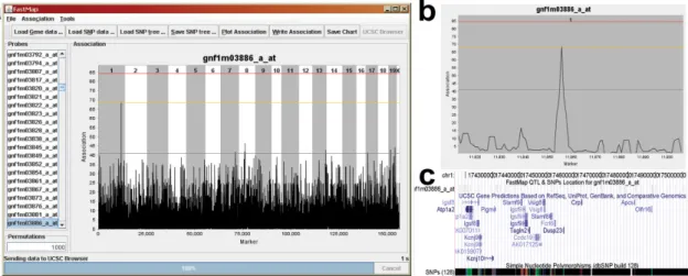
FastMap is written in the Java programming language and is driven by a simple graphical user interface (GUI, Figure 2.2a). The required input files are 1) a transcript expression file with mean expression values for each mouse strain and 2) a SNP file containing allele calls for all strains, with the major and minor alleles coded as 0 and 1 respectively. Once the SNP file has been loaded, FastMap constructs a Subset Summation Tree (see Methods) for the SNP data, a computational task that is performed only once for a given set of strains. FastMap allows the user to perform either SMM by calculating the Pearson correlation of each transcript expression measurement with each SNP, or HAM by sliding an m-SNP window across the genome and calculating the ANOVA F-statistic for the phenotype vs. the distinct haplotypes observed in the window (Pletcher et al. 2004). The
23
association statistic at each SNP is displayed in a zoomable panel that links to the University of California at Santa Cruz Genome Browser (Kent et al. 2002) (Figure 2.2b & c). Association plots may be exported as text files or as images.
QTL mapping with sparsely distributed markers has traditionally used Maximum Likelihood methods and has employed the Likelihood Ratio Statistic (LRS) or the related Log of the Odds ratio (LOD) as a measure of the association between genotype and phenotype (LRS = 2 ln(10) x LOD). When marker density is high, regression techniques applied only at the observed markers will produce results which are numerically equivalent to the LRS or LOD (Kong and Wright 1994). In fact, the LRS, Student t-statistic, Pearson correlation and the standard F-statistic, can be shown to be equivalent when they are applied at the marker locations. While previous literature has shown that regression methods produce estimates with a higher mean square error and have less power (Kao 2000), these results apply primarily to the case of interval mapping when the spacing between markers is wide (> 1cM). For these reasons, FastMap employs the Pearson correlation for SMM and the F-statistic for HAM when employing high density SNP data sets.
24
for any choice of these statistics. Once a QTL peak that exceeds a user selected threshold has been identified, the width of the QTL must be defined in order to identify potential candidate genes for further study. Given a local maximum d, a confidence region can be defined as all markers q in an interval around d such that 2 ln(LR(q)) ≥ maxd 2 ln(LR(d)) - x and this interval is referred to as an (x/2 ln 10)-LOD support interval (Dupuis and Siegmund 1999). The choice of x = 4.6 yields a 1-LOD confidence interval, which has been widely used in linkage analysis. A more conservative choice of x = 6.9 (a 1.5-LOD interval) is more appropriate to situations with dense markers, yielding approximate 95% coverage under dense marker scenarios. Intervals for non-LR association statistics can be calculated from the relationships between association statistics. In practice, eQTL peak regions are limited by the effective resolution determined by breeding and recombination history.
25
Permutation based significance testing is frequently used in eQTL analysis (Doerge and Churchill 1996; Peirce et al. 2006), and typically forms the bulk of the computational burden in eQTL mapping. It is natural to ask whether a parametric approach, based on Gaussian p-values, would be just as effective and save a significant amount of time. We note that permutation based testing offers several advantages over parametric approaches. Permutation testing deals cleanly with the problem of multiple comparisons, and induces a null distribution under which there is no association between transcript expression and genotype, regardless of the underlying distributions from which the data are drawn, and the correlations between SNPs. In addition, the normality assumptions underlying parametric tests are often violated in practice.
Performance and Speed
26
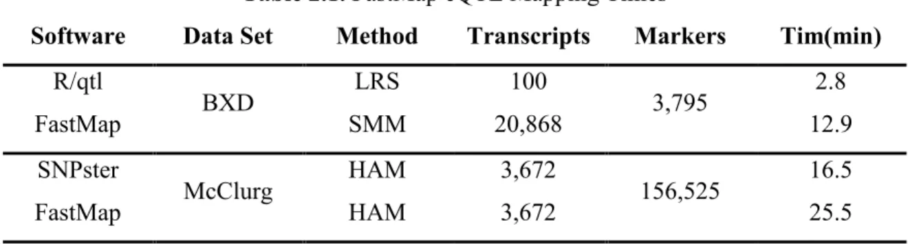
Table 2.1. FastMap eQTL Mapping Times
Software Data Set Method Transcripts Markers Tim(min) R/qtl
BXD LRS 100 3,795 2.8
FastMap SMM 20,868 12.9
SNPster
McClurg HAM 3,672 156,525 16.5
FastMap HAM 3,672 25.5
27
reasonable amount of time (overnight, or over a weekend for more than ten thousand transcripts).
We evaluated the scalability of FastMap with increasing numbers of transcripts and SNPs using the hypothalamus data set. Since we are aware of no stand-alone software that can perform eQTL mapping with hundreds of thousands of SNPs, we compared FastMap’s performance in these plots to a brute force approach in which all calculations are performed without any optimizations. In the case of both SMM and HAM, computation time for FastMap scales linearly with increasing numbers of transcripts (Figure 2.3a). FastMap also scales linearly with increasing number of SNPs (Figure 2.3b).
In order to examine the scalability of our algorithm with increasing numbers of
28
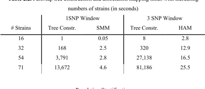
to each other. As more distantly related strains are added (i.e. M.m.domesticus derived strains combined with M.m.musculus derived strains), the distance between SDPs becomes larger and tree construction times increase. Most existing eQTL studies in panels of inbred strains have used less than 40 strains (Bystrykh et al., 2005; Chesler et al., 2005; McClurg et al., 2007). Tree construction required 5.3 minutes for the 32 strains of the hypothalamus data set. In contrast, for a panel of 71 inbred strains derived from both M.m.domesticus and non-M.m.domesticus strains, tree construction requires ~10 hours using a 1 SNP window and ∼24 hours using a 3 SNP window. Tree construction is carried out only once, and the resulting calculations still require less time than a brute force approach. Faster algorithms for tree construction that improve scalability with increasing numbers of strains are currently under investigation.
Table 2.2. FastMap tree construction and association mapping times with increasing numbers of strains (in seconds)
1SNP Window 3 SNP Window
# Strains Tree Constr. SMM Tree Constr. HAM
16 1 0.05 8 2.8
32 168 2.5 320 12.9
54 3,791 2.8 27,138 16.5
71 13,672 4.6 81,186 25.5
Population Stratification
29
30
31
within strata or the non-uniform resampling technique used by SNPster should not be required.
Comparison of FastMap to other QTL software
We compared the eQTL results produced by FastMap to those produced by R/qtl. R/qtl was configured to use Haley-Knott regression (Haley and Knott 1992) and 1,000 permutations to determine significance thresholds. While R/qtl is designed to perform linkage mapping, we note that when linkage mapping is performed exclusively at the markers, the calculations are identical to those performed in eQTL. eQTLs may be broadly separated into two categories; eQTLs located within 1Mb of the transcript location (cis-eQTLs), and eQTLs located further than 1 Mb from the transcript location (trans-eQTLs). Both FastMap and R/qtl found similar numbers of total eQTLs, ciseQTLs and trans-eQTLs (Figure 2.6a). Figure 2.6b shows that the eQTL locations found by each software package are essentially identical; 98% of the eQTLs found by each method are within 5 Mb of each other, a margin of resolution consistent with the resolution of the BXD marker set. Since permutation based testing involves randomization, it should not be expected that 100% of the eQTLs would match between the two methods. Furthermore, the eQTL histograms produced by each method (Figure 2.6c & d) are similar, with differences being due to histogram binning effects (see insets).
32
33
34
Since SNPster does not provide a fixed threshold for significance, we selected 2,413 transcripts which had SNPster p-values less than 10-4. Of these, 105 were cis-eQTLs and 2,308 were trans-eQTLs. FastMap produced eQTLs for 382 transcripts at or above a 0.05 significance threshold, of which 29 were cis-eQTLs and 353 were trans-eQTLs. The locations of 55 eQTLS were common between the two methods and all of these were
35
eQTLs, which have been reported to be more reproducible than trans-eQTLs (Peirce et al. 2006).
It should be noted that FastMap and SNPster differ in several important respects. SNPster uses a heuristic weighted F-statistic who’s null distribution is not known, it employs a resampling approach that selects strains in a random manner with a nonuniform distribution. FastMap uses the standard F-statistic and conventional permutation-based significance thresholds. For these reasons, it is unclear whether the results of the two methods should be concordant, and biological validation of both eQTL mapping approaches may be necessary to address the differences.
Conclusion
Chapter 3
Genome-level analysis of genetic regulation of liver gene expression networks
Introduction
With the recent sequencing of entire mammalian genomes (Venter et al. 2001; Waterston et al. 2002), the possibility exists that the genetic basis of liver injury can be unraveled. Several high density genotyping projects are underway to sequence panels of inbred strains at densities of ~150,000 and ~8.3 loci (Lindblad-Toh et al. 2000; Sherry et al. 2001), providing an unprecedented density of genomic information. This detailed sequence data can be combined with high throughput gene expression microarrays to examine the effect of genetics on constitutive levels of gene expression (Schadt et al. 2003; Chesler et al. 2005; Bystrykh et al. 2005). The combination of such high dimension data sets can offer insight into complex mechanisms of liver disease and toxicity (Schadt 2005).
37
(Watkins and Seeff 2006). These properties make idiosyncratic liver injury extremely difficult to predict. Further, if such reactions occur when patients are intentionally exposed to drugs, it is possible that environmental xenobiotics can have the same effects. While most of the population does not experience an adverse response to common environmental exposures, a small percentage may experience an idiosyncratic response. An increased understanding of the mechanisms of toxicity in the liver will allow us to better predict and prevent such incidents.
All human populations are exposed to environmental toxins and toxicants. However, the response to such exposures is not uniform. While the majority of the population may experience exposure and suffer no measurable injury, a minority may experience severe toxicity. The reasons for such differential responses are many. Exposure dose and duration, lifestyle and nutritional choices, genetic differences and other variables can all affect the response. In this study, the focus is specifically on the genetic differences that influence the differential response to toxic insult.
38
In order to study the effect of genetic background on gene expression, mice with a controlled genotype are used. Inbred strains are homozygous at all genomic loci and whose individuals have identical genotypes. These strains are developed through extended sibling mating for over 20 generations. This process leads to increased homozygosity over at least 99% of the genome. The use of inbred strains in genetics is well established and some strains have been bred and used in laboratory experiments for almost 100 years (Wade and Daly 2005). The decreased genetic diversity within a single inbred strain leads to greatly reduced phenotypic variance, reducing the number of mice needed to detect statistically significant phenotypic differences. The stable genotype is also invaluable for reproducing phenoptypic measurements in different laboratories. Environmental factors can be varied in a controlled manner without additional genotypic variation (Paigen and Eppig 2000). It is important to note that while the phenotypic variation within an inbred strain is reduced, the phenotypic variation among a panel of inbred strains can remain vast (Svenson et al. 2007).
39
Quantitative Trait Locus (QTL) mapping has been used to associate a specific genotype with the variation in a single measured phenotype like high density lipoproteins (Wang and Paigen 2005) and ethanol tolerance (Grisel et al. 2002). At each locus in a segregating population, a model is fit which estimates the likelihood that this locus explains the variation in phenotype versus the likelihood that there is no genotypic effect on the phenotype.
Interval mapping (Lander and Botstein 1989) is a variation on QTL mapping which uses maximum likelihood estimation. At each marker, the likelihood that the marker is associated with the phenotype over the likelihood that the marker is associated with no genotype is calculated. This is the Likelihood Ratio Statistic (LRS). Between markers, the exact genotype is unknown. Because of this missing data, the expectation maximization algorithm is used to estimate the genotype based on recombination frequencies. The result is a QTL plot of the entire genome with LRS scores indicating the strength of association between the phenotype and each genomic location.
40
This approach has been applied in the mouse liver (Schadt et al. 2003),brain (Chesler et al. 2005) and hematopoetic stem cells (Bystrykh et al. 2005). The liver study (Schadt et al. 2003) used an F2 population derived from C57BL/6J and DBA/2J to study the relationship of liver gene expression to fat pad mass. The others (Chesler et al. 2005; Bystrykh et al. 2005) looked at constitutive gene expression in a panel of BXD RI mice to infer the regulation of basal gene expression. These studies were significant in increasing our understanding gene regulatory networks including the existence of master regulator loci, clusters of co-regulated genes and the association of gene expression with previously measured behavioral traits.
Missing from the current literature is a study of constitutive gene expression in the mouse liver using a panel of RI strains. Such a study would lay a foundation of basic research for liver toxicologists and provide a resource which can be used to associate genes expression with phenotype measurements. It could be used to find clusters of co-regulated genes that may not have been otherwise associated in previous work and to build regulatory networks for genes relevant to xenobiotic metabolism. Lastly, such a data set could be used for intelligent strain selection when a knockout model is otherwise unavailable.
41
in transcript expression to phenotypes. However, they do not lead to detailed gene expression networks where the expression of one gene is found control the expression of another.
Recombinant Inbred (RI) mice are created by crossing two parental strains followed by sib-mating for over 20 generations (Taylor 1989). Strains created this way have the advantage of being homozygous at almost every location along the genome. As such, each representative of an RI line will have limited phenotypic variation within that line, but the variation between lines is usually vast. RI panels are widely used to determine genotype-phenotype associations using QTL mapping techniques (Lander and Botstein 1989). The relationships between phenotypes and genotypes are calculated using a likelihood ratio statistic (LRS), which is a measure of the probability that a given genetic marker explains the variation in the phenotype. When mRNA levels are used as the phenotype, regions of the genome with a high LRS are likely to contain genes that control the expression of the gene transcript being profiled; this process is referred to as expression Quantitative Trait Loci (eQTL) mapping (Schadt et al. 2003; Farrall 2004).
42
BXD mice were used for eQTL studies that elucidated the genetics of gene expression in the brain (Chesler et al. 2005) and hematopoietic stem cells (Bystrykh et al. 2005).
43 Methods
Animals and Tissues. BXD1 through BXD42 mice are original RI strains available from the Jackson Laboratory (Bar Harbor, ME). BXD43 through BXD100 lines were generated using ninth or tenth generation Advanced Intercross Line (AIL) progenitors. AILs are generated by breeding two inbred parents (here is C57BL/6J and DBA/2J) and crossing their offspring so as to minimize inbreeding and maximize recombination events at each generation (Peirce et al. 2004). Mice were maintained at 20-24°C on a 14/10 hr light/dark cycle in a pathogen-free colony at the University of Tennessee-Memphis. Animals were fed a 5% fat Agway Prolab 3000 rat and mouse chow and given tap water in glass bottles. Strain details are provided in Appendix 1. Mice were raised to between 54 and 177 days (mean 70 days) of age. Liver tissues were collected following sacrifice by cervical dislocation. The whole liver was removed immediately, and placed in five volumes of RNAlater (Ambion, Austin, TX) at 4°C overnight, before removing from RNAlater and storing at -80°C until processing. All animal studies for this project were approved by Animal Care and Use Committee at the University of Tennessee-Memphis.
44
45
Inter-batch normalization was carried out using a nested ANOVA mixed model with samples within each batch crossed with sex and strain.
QTL Analysis and WebQTL. QTL linkage mapping was carried out using the QTL Reaper software package (qtlreaper.sourceforge.net). One thousand permutations of the strain labels were performed to estimate the genome wide p-value (Churchill and Doerge 1994). Liver expression data was deposited in WebQTL (www.genenetwork.org) which is a web-based resource for exploring gene expression and phenotype interactions. WebQTL was used to produce interval maps for specific genes.
46
Transcription Factor Analysis. Three web-based tools were used to search for possible
transcription factor binding sites in candidate loci: the National Cancer Institute’s Advanced Biomedical Computing Center promoter analysis tool (grid.abcc.ncifcrf.gov/promoters.php), oPossum version 1.3 (Ho Sui et al. 2005) and PAINT (Vadigepalli et al. 2003). In the first two cases, transcripts were divided based on increased expression correlating with the C57BL/6J of DBA/2J allele. The transcripts were submitted in 4 groups: 1) high expression with the C57BL/6J allele and an LRS of 30 or greater, 2) high expression with the C57BL/6J allele and an LRS of 40 or greater, 3) high expression with the DBA/2J allele and an LRS of 30 or greater and 4) high expression with the DBA/2J allele and an LRS of 40 or greater. With PAINT, all transcripts were submitted as one list, but a gene cluster file was also submitted that clustered the C57BL/6J high and DBA/2J high transcripts into separate clusters.
47
280 nm wavelengths. 20 µg of RNA were used to produce cDNA using the Applied Biosystems Inc. (Foster City, CA) High Capacity cDNA Archive Kit. The Stratagene (La Jolla, CA) FullVelocity QYBR Green QPC Master Mix was used to perform the RTPCR and the plates were run on a Stratagene Mx3000P instrument.
Results and Discussion
Genetic control of gene expression in liver
48
49
50
To visualize the patterns of genetic control of gene expression on a genome-wide level, the 18716 annotated transcripts were clustered using the LRS vector for each transcript (Figure 3.2a). As expected, the majority of the transcripts in liver are independently regulated; however, several distinct patterns emerge. Specifically, there are a number of clusters of transcripts that all share a common maximal QTL as well as clusters that are co-regulated by a complex set of common loci. We refer to clusters co-regulated by only one strong QTL as “simple” QTL clusters and ones regulated by multiple loci as “complex” clusters.
Chromosome 8 contains a simple cluster of transcripts that all have a strong maximum QTL (mean LRS = 47.5, Figure 3.2b). Of the 27 transcripts in this cluster, 26 are located on chromosome 8 at the same location as the maximum QTL which indicates that this cluster contains predominantly cis-regulated genes or perhaps is due to a strain-specific difference in a regional transcriptional enhancer. Interestingly, the presence of one of the parental (C57BL/6J or DBA/2J) allele at this locus strongly affects expression of these genes (Figure 3.2b, yellow-red correlation plot).
51
52
53
Lastly, a cluster of 43 transcripts (Figure 3.2d) that are controlled by a complex pattern of loci across multiple chromosomes (mean maximum LRS = 13.3) is shown. Not surprisingly, these genes are scattered around the genome. The pair-wise gene expression correlation matrix for these transcripts shows that mRNA levels for these genes are highly positively correlated regardless of the allele type at each QTL.
54
Mouse brain and liver transcriptomes show little overlap in genetic regulation of gene expression
Several recent reports identified a number of master-regulatory loci in other mouse tissues (Chesler et al. 2005; Bystrykh et al. 2005; Peirce et al. 2006). Here, the mouse brain (forebrain) and liver transcriptome maps (Figure 3.3) are compared to uncover the similarities and differences in genetic regulation of gene expression across tissues. Both brain and liver contain genes that are strongly cis- or trans- regulated at single loci, or are regulated by multiple loci (Figures 3.3a and b, respectively). In the brain transcriptome, three distinct master-regulator trans-bands are located on chromosomes 1 and 2 (Figure 3.3c). In the liver transcriptome, the strongest trans-band is located on distal chromosome 12 (Figure 3.3d), a locus that does not appear to be controlling expression of a large number of genes in the brain. While the liver and the brain both have a trans-band on chromosome 2 near 125 Mb, the two bands are not coincident. The liver trans-band lies at 119 MB and the brain at 135 Mb - a difference of 16 Mb.
55
56
57
Chromosome 12 contains a strong liver-specific master-regulatory locus
58
59
It was reasoned that the candidate gene that may be responsible for the variation in expression between the transcripts associated with this locus should satisfy the following properties: 1) be cis-regulated at the chromosome 12 locus or contain non-synonymous coding SNPs between parental alleles, 2) have median to high expression in liver and 3) exhibit strong correlation in gene expression between the candidate gene and the trans-regulated transcripts when separated by parental allele at this locus. Five genes that are located in this region are cis-regulated: Dicer1, Serpina3k, Serpina3n, Serpina9 and Serpina12 (Figure 3.4, middle panel, genes identified in italics). Furthermore, a number of genes in this region, including Serpina3k, Serpina3n, Serpina9, and Serpina12, have known non-synonymous coding SNPs between the C57BL/6J and DBA/2J strains. Serpina3k, Serpina3n, Dicer1, Serpina9 and Serpina12, among several other genes, also have median to high relative mRNA expression in liver. Lastly, when the strength of the correlation between expression of each transcript regulated by this locus and expression of all other transcripts located in the chromosome 12 locus is plotted (Figure 3.4, top panel), it is evident that Dicer1, Serpina3k, Serpina3n, Serpina9, Serpina12 andfour other transcripts have a clear separation (positive or negative correlation) according to the parental strain allele at this locus. Thus, it appears that any of the 5 cis-regulated genes at this locus: Dicer1, Serpina3k, Serpina3n, Serpina9, Serpina12 is likely to be the candidate "master regulator" gene in liver.
60
date, no specific gene regulatory function has been proposed for Dicer1 in the liver. To test the hypothesis that Dicer1 is a master-regulator of gene expression in the liver, expression was compared between the chromosome 12 locus-regulated genes in livers of wild type and Dicer1 heterozygous [Dicer1 null mutation is embryonic lethal (Bernstein et al. 2003)] mice by quantitative real time PCR. As a negative control, a number of randomly selected genes that are not regulated by the chromsome12 locus were selected. Contrary to our hypothesis, no consistent correlation was found between expression of Dicer1 and chromosome 12 locus-regulated genes (data not shown) which suggests that Dicer1 does not appear to be the master regulator at this locus. It should be noted, however, that Dicer1 heterozygous mice may not be the most appropriate system for testing this hypothesis since Dicer1 mRNA levels in heterozygotes are 134% of wild type levels and a small sample size (n = 3 per group) limits the power of the analysis (p = 0.17).
Next, other means of biological interpretation of the data were considered. Gene Ontology (GO) and transcription factor binding site analyses of the chromosome 12 locus trans-regulated genes were performed. GOMiner (Zeeberg et al. 2003) examination of the 111 transcripts with maximum QTLs at the chromosome 12 locus identified significant enrichment for a single biological process category – cell surface receptor linked signal transduction (p=8.74x10⁻⁴). The genes from this category that are trans-regulated by the chromosome 12 locus are mainly olfactory receptors: Bsf3, Rqcd1, Gpr50, Tcp10c, P2ry10, Olfr1403, Olfr1443, Olfr401, Olfr512, Olfr935, Olfr1341, Olfr341, Olfr656, Olfr1365,
Mesp2, Met, Ltbp3, Fstl3, Centd2, and Rassf3.
61
those with high expression when either C57BL/6J or DBA/2J allele is present at the chromosome 12 locus. The National Cancer Institute’s Advanced Biomedical Computing Center promoter analysis tool (grid.abcc.ncifcrf.gov/promoters.php) found no common transcription factor binding sites for the C57BL/6J list. LVc-Mo-MuLV and SV40.11 binding sites were identified as significant (p = 9.766e-04) in the DBA/2J list. The oPossum (Ho Sui et al. 2005) tool identified Freac-2 site as significant in both C57BL/6J and DBA/2J lists (p = 6.026e-02 and p = 1.823e-02, respectively), while ARNT (p = 8.577e-02) and SOX-9 (p = 9.159e-02) sites were also found to be common for DBA/2J allele-containing genes. The PAINT transcription factor tool (Vadigepalli et al. 2003) was also applied to the data and no significant transcription factor binding sites between the two lists were found after FDR correction of the p-values. Similarly to our observation of the lack of a consistent signal for a transcription factor, (Yvert et al. 2003) and (Kulp and Jagalur 2006) found that the genes in trans-regulated bands are not enriched for transcription factors or biological function. This suggests that the trans-regulated genes at the chromosome 12 locus have a complex mechanism of regulation that is yet to be discovered.
62
α1-Anti-chymotrypsin has been shown to be present in the amyloid plaques of Alzheimer’s patients (Forsyth et al. 2003). Elzouki et al. (Elzouki et al. 1997) found an association between low plasma α1-anti-chymotrypsin levels and propensity to contract the hepatitis B
& C virus. A related protease inhibitor, serpina1 (α1-antitrypsin) is involved in emphysema due to a failure to inhibit neutrophil elastase and cirrhosis due to an accumulation of serpina1 polymers in the hepatocytes (Janciauskiene 2001; Perlmutter 2006). Although the overall structure is well conserved in the 14 member mouse Serpina3 family, the reactive center loop is widely divergent, suggesting that these enzymes have function other than protease inhibition. Interestingly, human α1-anti-chymotrypsin was reported to be able to bind to DNA and has been found to inhibit DNA polymerase and DNA primase in vitro (Janciauskiene 2001). Horvath et al. (Horvath et al. 2005) performed a detailed structural analysis of mouse SERPINA3N and found that it contains a DNA binding domain similar to one described in human α1-anti-chymotrypsin (Naidoo et al. 1995). However, it was also
63
eQTL analysis facilitates the discovery of novel genotype-phenotype correlations
WebQTL contains comprehensive manually curated publicly available data for phenotypic and gene expression profiling of a number of recombinant inbred and F2 crosses in both mouse and rat along with the dense genetic marker maps for these strains. Thus, this data can be used to search for correlations between phenotypes, gene expression and genetic markers, i.e., to perform in silico genotype-phenotype association analysis. The inherent significance of the defined reference genetic populations, such as BXD RI strains, is in the ability to connect historical data generated in many laboratories to the exact genetic map of each strain. This provides an exceptional opportunity to add value and depth to the biological interpretation of the data from model organisms. Thus, even though the BXD RI panel of strains has not been used extensively to profile liver disease-specific responses, as compared to a wealth of behavioral phenotypes published over the years, it is not unreasonable to anticipate that more data will become available soon.
64
TNF injection (Libert et al. 1999). Furthermore, both the expression of Hnf4g and values of these phenotypes separate by parental allele at the location of the Hnf4g gene on proximal chromosome 3.
Knowledge of the variability in basal gene expression in liver as a tool for selecting relevant strains to probe biology
65
Furthermore, some genes are embryonic lethal while others are sufficiently redundant, thus limiting the ability to generate biologically meaningful data using genetic engineering approaches. Thus, we propose that understanding of the degree of variability in gene expression between strains in a reference population of mice may be used to model the potential biological effects of naturally occurring differences in mRNA levels between individuals. In fact, it is extremely rare that people are complete nulls for a particular gene, but the polymorphisms in certain genes are known to predispose the individuals to some exposures or lead to disease (Dolphin et al. 1997; Rudnick and Perlmutter 2005). Accordingly, the liver expression data in WebQTL may be utilized to select strains that differ in basal mRNA level of genes of interest and then used for phenotypic studies that are designed to test the role of the genes in a particular phenotype.
66
strains and mutations in this gene have been implicated in trimethylaminuria (Dolphin et al. 1997), a disease in which trimethylamine is not metabolized but is excreted in the breath and sweat, leading to a persistent fishy body odor, we suggest that BXD strains with high or low relative expression of Fmo3 may be used to model this disease. Similar logic may be used to test other genes without the cost and time of generating knockout animals.
Conclusions
67
Chapter 4
Sex-specific Gene Expression in the BXD Mouse Liver
Introduction
Physiological differences between the sexes have their roots in sexually dimorphic levels of gene expression (Mode and Gustafsson 2006; Waxman and Holloway 2009b). Despite containing identical autosomes and differing by a single Y chromosome, genes exhibiting expression differences are broadly distributed throughout the genome. In the liver, many of these differences are driven primarily by the pituitary growth hormone (GH) (Waxman and O'Connor 2006) which acts through the signal transducer and activator of transcription 5b (STAT5b) (Clodfelter et al. 2007; Holloway et al. 2007) and hepatocyte-enriched nuclear factor (HNF4α) (Holloway et al. 2008). These transcription factors, through direct and indirect mechanisms, are thought to regulate expression of many steroid and xenobiotic metabolizing enzymes, leading to observed patterns of sexually dimorphic expression in a number of important biological pathways (Waxman and Holloway 2009b).
69
Cyp4a12, Hsd3b5m, Elovl3 and Keg1. (Clodfelter et al. 2006) studied liver gene expression changes in Stat5b knockout and wild type mice, finding 1,603 differentially regulated genes, with 850 being male- and 753 female-biased (p<0.05 and FC>1.5). A large study consisting of 344 mice comprising an F2 cross between C57B/6J.apoE-/- and C3H/HeJ.apoE-/- strains (~50% from each sex) produced two reports (Wang et al. 2006; Yang et al. 2006) which examined sexually dimorphic gene expression in adipose tissue, brain, liver and muscle. It was reported that 9,250 genes are dimorphic in the liver (p<0.01 and FC>1). In an effort to uncover regulatory pathways driven by genetic variation, the authors also performed gene expression quantitative trait locus (eQTL) mapping to find genomic loci responsible for transcriptional regulation of clusters of genes. The authors reported that one locus on medial Chr 5 regulated the expression of ~80 genes and the genes in this cluster were enriched for cell cycle, cell proliferation and DNA replication. While these, as well as other previous investigations into sexual dimorphism of specific genes in liver made crucial contributions to knowledge of sex-specific gene expression patterns in liver, their goals were either tissue comparisons (Rinn et al. 2004; Yang et al. 2006), discovery of the transcriptional response to loss of Stat5b (Clodfelter et al. 2006), or characterization of the obesity phenotypes (Wang et al. 2006; Yang et al. 2006).
70
71 Methods
Gene Expression Data. The details of mouse breeding, housing, RNA isolation and gene expression are described elsewhere (Gatti et al. 2007). Tissue collection (synchronized with respect to the time of day) was conducted at the University of Tennessee at Memphis and approved by the Institutional Animal Care and Use Committee. Briefly, gene expression in the livers of 37 strains of male and female C57BL/6JxDBA/2J (BXD) recombinant inbred (RI) mice, the C57BL/6J and DBA/2J parentals, and the C57BL/6JxDB2/2J F1 generation (B6D2F1) mice was measured using the Agilent (Santa Clara, CA) G4121A microarray (20,868 transcripts). The data was normalized by taking the fitted values from a nested, mixed model consisting of batch, strain, sex and strain by sex interaction terms. Additional details regarding animals, microarrays, data acquisition, processing and analyses can be found at WebQTL.org (http://webqtl.org/dbdoc/LV_G_0106_B.html). The data has been deposited in the Gene Expression Omnibus (GSE17522).
72
Significant categories were selected based on q-values of ≤0.25, a 25% FDR for the entire list.
Sex Specific Correlated Gene Clusters: The Spearman correlation of each transcript with all 20,867 other transcripts on the array was calculated for males and females independently. Transcripts with correlations ≥0.7 in either males, or females were retained separately for each transcript as highly correlated clusters. Gene sets with absolute mean differences in correlation between sexes ≥0.35 were selected as sex-specific correlated clusters. Both cutoffs were selected to produce reasonably short lists of interpretable results. The highly correlated sex-specific gene clusters from the above analysis were searched for GO and KEGG pathway enrichment using Fisher’s Exact Test. Significant categories were selected with q-values ≤0.1.
Transcription Factor Binding Site Enrichment: The Opossum single site analysis algorithm (Ho Sui et al. 2007) was used to query the JASPAR vertebrate database for enrichment in transcription factor binding sites (TFBS). The selected parameters, in the order they appear on the web site were 1) Level of conservation: top 10% of conserved regions, 2) Matrix match threshold: 80%, 3) Amount of upstream/downstream sequence: -5000/+5000, 4) Results: Z-score > 10 and Fisher score < 0.01.
Gene Expression Quantitative Trait Locus Mapping. eQTL mapping was performed using single marker mapping in FastMap (Gatti et al. 2009b), which uses sample permutation to produce per-gene significance thresholds. Mapping was performed on all 20,868 transcripts represented on the array and a set of 3,795 markers downloaded from WebQTL
73
74 Results
Characterization of Sexually Dimorphic Liver Genes in BXD Mouse Panel
Sexually dimorphic genes were selected using a two-way (sex and strain of each sample) Analysis of Variance (ANOVA) model. P-values for sex and strain were filtered separately using q-values (Storey and Tibshirani 2003) of 0.01, 0.05 and 0.1, which represent the False Discovery Rate (FDR) of the resulting gene lists, corresponding to FDRs of 1%, 5% and 10%. At the highest q-value, we find a similar number of dimorphic genes as a previous report (Yang et al. 2006) and replicate the finding that there are more female-biased genes than male-biased genes (Table 4.1). To further explore the differences, we plotted the mean expression value for each gene in males versus that in females (Figure 4.1) and observed that, while there are more febiased genes, there is also a large cluster of male-biased genes (Figure 4.1, circle). The genes in this cluster (q≤0.01, 0≤male≤2.6,
-0.5≤female≤1.5) are significantly enriched for olfactory receptor activity (GO:0004984, p=9.6x10⁻²²) which consists of G-protein coupled receptors involved in signaling.
Table 4.1. The number of sexually dimorphic genes in the BXD mouse liver.
q-value p-value Male-biased Female-biased Total
BXD
recombinant inbred panel
0.01 0.0048 2,250 3,066 5,316
0.05 0.0342 3,048 4,495 7,593
0.10 0.0821 3,709 5,393 9,102
75
As expected, some of the most sexually dimorphic genes (Table 4.2) are located on the X and Y chromosomes, including inactive X specific transcripts (Xist), DEAD box polypeptide 3, Y-linked (Ddx3y), and eukaryotic translation initiation factor 2, subunit 3, structural gene Y-linked (Eif2s3y). However, most genes that exhibit considerable fold difference in expression (>2) between sexes reside on autosomes. We have compared our results to two independent microarray studies that examined sex differences in liver gene expression in mice. We compared our study with that of (Clodfelter et al. 2006) which was conducted on Stat5b-null and wild type mice. We used a rather conservative p≤0.01 cut-off for sex bias and found overlap of 51.5% (410 out of 796 genes from that study matched with an identical p-value). A similar comparison with a study which used an a much larger number of mice in an F2 cross (Yang et al. 2006) yields a 27.2% overlap (9,250 genes were reported as sexually dimorphic with p≤0.01, of which 8,087 mapped to Agilent 4121A microarray and 2,196 matched our results).
76