LOW LATENCY DISPLAYS FOR AUGMENTED REALITY
Peter C. Lincoln
A dissertation submitted to the faculty of the University of North Carolina at Chapel Hill in partial fulfillment of the requirements for the degree of Doctor of Philosophy in the Department of Computer Science.
Chapel Hill 2017
ABSTRACT
Peter C. Lincoln: Low Latency Displays for Augmented Reality (Under the direction of Henry Fuchs and Greg Welch)
The primary goal for Augmented Reality (AR) is bringing the real and virtual together into a common space. Maintaining this illusion, however, requires preserving spatially and temporally consistent registration despite changes in user or object pose. The greatest source of registration error is latency—the delay between when something moves and the display changes in response—which breaks temporal consistency. Furthermore, the real world varies greatly in brightness; ranging from bright sunlight to deep shadows. Thus, a compelling AR system must also support High-Dynamic Range (HDR) to maintain its virtual objects’ appearance both spatially and temporally consistent with the real world.
This dissertation presents new methods, implementations, results (both visual and performance), and future steps for low latency displays, primarily in the context of Optical See-through Augmented Reality (OST-AR) Head-Mounted Displays, focusing ontemporal consistency in registration,HDR color support, andspatial and temporal consistency in brightness:
1. Forregistration temporal consistency, the primary insight is breaking the conventional display paradigm: computers render imagery, frame by frame, and then transmit it to the display for emission. Instead, the display must also contribute towards rendering by performing a post-rendering, post-transmission warp of the computer-supplied imagery in the display hardware. By compensating in the display for system latency by using the latest tracking information, much of the latency can be short-circuited. Furthermore, the low latency display must support ultra-high frequency (multiple kHz) refreshing to minimize pose displacement between updates.
LEDs illuminators at frequencies to support kHz-order HDR exceeds their capabilities. Thus one must directly synthesize the necessary variation in brightness.
ACKNOWLEDGMENTS
First, I would like to thank my advisors Henry Fuchs and Greg Welch, whom have guided me and supported me through all these years. I would also like to thank my other committee members for their support and advice: Oliver Bimber, Anselmo Lastra, Montek Singh, Bruce Thomas, and Turner Whitted.
In my time at UNC, I have worked on several papers, both on this thesis’ topic and others, and I would like to thank my co-authors as well: Alex Blate, Juan Cendan, David Chesnutt, Henry Fuchs, Adrian Ilie, Anselmo Lastra, Andrew Maimone, Arjun Negendran, Andrew Nashel, Remo Pillat, Diego Rivera-Guiterrez, Ryan Schubert, Montek Singh, Andrei State, Herman Towles, Greg Welch, Turner Whitted, Mary C. Whitton, and Feng Zheng. I would also like to thank the other people who helped on projects related to those papers or other Research Assistantship (RA) work, including Jonathan Bidwell, Mingsong Dou, Yinan Fang, Jan-Michael Frahm, Zachary Kaplan, Mod Marathe, Bill Mauchly, and Ying Shi. I would also like to specifically thank Kurtis Keller, Jim Mahaney, John Thomas, and Herman Towles for their engineering support on each of my projects at UNC. I would also like to thank Alex Blate for collaborating on the Low Latency Displays project as well as designing and fabricating some of the electronics hardware necessary for making the display work. I would also like to thank the UNC Computer Science Department staff for administrative support over the years.
I would like to thank several people for sitting in on photos used in this thesis: Fay Alexander, Steve Partin, Brett Piper, and Hope Woodhouse in Figure 1.2; and Brett Piper in Figure 4.8.
While working as an RA for Henry Fuchs on the Low Latency Displays project, I have been funded by multiple sources, which I would like to thank:
• National Science Foundation Award CHS IIS-1423059: “Minimal-Latency Tracking and Display for Head-Worn Augmented Reality Systems,” Dr. Lawrence Rosenblum, Program Manager
Foundation under its International Research Centre @ Singapore Funding Initiative and administered by the Interactive Digital Media Programme Office.
• The BeingTogether Centre, a collaboration between Nanyang Technological University (NTU) Singapore and University of North Carolina (UNC) at Chapel Hill. The BeingTogether Centre is supported by the National Research Foundation, Prime Minister’s Office, Singapore, under its International Research Centres in Singapore Funding Initiative.
While working as an RA for Henry Fuchs and Greg Welch on other projects, I have been funded by multiple sources, which I would also like to thank:
• Multi-View Telepresence and Telepresence Wall – CISCO
• Avatar
– Office of Naval Research Award N00014-09-1-0813: “3D Display and Capture of Humans for Live-Virtual Training,” Dr. Roy Stripling, Program Manager
• Multi-Projector Blending
– Office of Naval Research Award N00014-09-1-0813: “3D Display and Capture of Humans for Live-Virtual Training,” Dr. Roy Stripling, Program Manager
PREFACE
This dissertation is primarily based on the following publications: Lincoln et al. (2016) and Lincoln et al. (2017), which have appeared in the indicated peer-reviewed journal or conference proceedings:
1. Lincoln, P., Blate, A., Singh, M., Whitted, T., State, A., Lastra, A., and Fuchs, H. (2016). From motion to photons in 80 microseconds: Towards minimal latency for virtual and augmented reality. IEEE Transactions on Visualization and Computer Graphics, 22(4):1367–1376
TABLE OF CONTENTS
LIST OF TABLES . . . xiii
LIST OF FIGURES . . . xiv
LIST OF ABBREVIATIONS . . . xvi
1 INTRODUCTION . . . 1
1.1 Vision . . . 1
1.2 Motivation . . . 2
1.2.1 Latency . . . 3
1.2.2 Dynamic Range . . . 4
1.3 Thesis Statement . . . 5
1.4 Contributions . . . 5
1.5 Structure . . . 6
2 BACKGROUND . . . 7
2.1 Introduction. . . 7
2.1.1 Units . . . 7
2.2 Related Work . . . 7
2.2.1 Existing Near-Eye OST-AR Displays . . . 7
2.2.2 Registration Error . . . 9
2.2.3 Latency Requirements . . . 9
2.2.4 Latency Mitigation Strategies . . . 10
2.2.4.1 GPU Improvements . . . 10
2.2.4.3 Post-Rendering Warp . . . 12
2.2.5 High-Dynamic Range . . . 13
2.3 DMD Operations . . . 14
2.3.1 DMD Chip Basics . . . 14
2.3.2 Conventional DMD Projector Basics . . . 15
2.4 Modulation . . . 16
2.4.1 Pulse Width Modulation . . . 17
2.4.2 Pulse Density Modulation . . . 17
3 LOW LATENCY RENDERING . . . 20
3.1 Introduction. . . 20
3.1.1 Contributions . . . 21
3.2 Render Cascade Pipeline . . . 21
3.3 Prototype: Simplified Render Pipeline . . . 23
3.3.1 Components and Implementation . . . 24
3.3.2 Visual Results: 6 bit/pixel Grayscale Implementation . . . 30
3.3.2.1 Experimental Setup . . . 30
3.3.2.2 Discussion . . . 31
3.3.3 Visual Results: 16 bit/color HDR Implementation . . . 33
3.3.4 Latency Analysis: 6 bit/pixel Grayscale Implementation . . . 33
3.3.4.1 Signal Path . . . 34
3.3.4.2 Measurement Instrumentation . . . 35
3.3.4.3 Latency Component Analysis . . . 36
3.3.4.4 Latency Range Analysis . . . 38
3.3.5 Latency Analysis: 16 bit/color HDR Implementation . . . 39
3.3.5.1 Signal Path . . . 40
3.3.5.2 Measurement Instrumentation . . . 40
3.3.5.4 Latency Range Analysis . . . 42
4 HIGH-DYNAMIC RANGE FOR LOW LATENCY DISPLAYS . . . 44
4.1 Introduction. . . 44
4.1.1 Contributions . . . 45
4.2 Display Scheme: Estimated Error Modulation . . . 45
4.2.1 Results . . . 46
4.2.2 Limitations . . . 46
4.3 Display Scheme: Pseudorandom Pulse Density Modulation . . . 48
4.3.1 Results . . . 50
4.3.1.1 Perceptual Comparison of PWM and PR-PDM . . . 51
4.3.2 Limitations . . . 53
4.4 Display Scheme: Direct Digital Synthesis . . . 53
4.4.1 Color Calibration . . . 55
4.4.2 Results . . . 57
4.4.3 Limitations . . . 60
4.5 Scene-Aware Spatial Brightness Control . . . 62
4.5.1 Results . . . 63
4.5.2 Limitations . . . 64
4.6 Summary . . . 67
5 SUMMARY AND CONCLUSIONS . . . 70
5.1 Summary . . . 70
5.2 Future Work . . . 71
5.2.1 Inertia . . . 71
5.2.2 Latency and General Pose Tracking . . . 72
5.2.3 Render Cascade Pipeline . . . 72
5.2.4 High(-er) Dynamic Range. . . 73
5.2.6 Video Latency . . . 75
5.2.7 Human Perception Studies . . . 75
5.2.8 Alternative Spatial Light Modulators . . . 76
5.3 Conclusions. . . 76
LIST OF TABLES
1.1 Example forms of error in AR systems . . . 3
3.1 Summary of latency components for the 6 bit/pixel system . . . 38
3.2 Summary of latency components for the 16 bit/color system . . . 43
4.1 Summary of color mixing parameters for the 16 bit/color system’s LEDs . . . 55
4.2 Computed color calibrated 16 bit/color DAC codes . . . 58
4.3 Comparison of modulation technique requirements . . . 68
4.4 Comparison of modulation technique behavior . . . 68
LIST OF FIGURES
1.1 The reality-virtuality continuum . . . 2
1.2 A sample scene of people in a room with HDR brightness . . . 5
1.3 A user “wearing” our AR display . . . 6
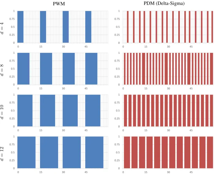
2.1 Sample comparison of simulated 4 bit gray level modulation schemes (PWM and Delta-Sigma) by method and desired intensity level . . . 18
3.1 A sample, conventional render pipeline . . . 21
3.2 Two sample PRW pipelines . . . 22
3.3 The PRW pipeline implemented in our prototype . . . 24
3.4 System assembly for the 6 bit/pixel system . . . 25
3.5 System assembly for the 16 bit/color system . . . 26
3.6 Implemented data path framework for image generation for the 6 bit/pixel grayscale system . . 27
3.7 Subset of implemented data path diagram for image generation for the 16 bit/color system . . . 28
3.8 A comparison between conventional displays and our latency compensation algo-rithm using the 6 bit/pixel mode . . . 32
3.9 A comparison between our latency compensation algorithm and a conventional display using the 16 bit/color mode . . . 34
3.10 Light measurement sensor and barrier . . . 35
3.11 Sample motion-to-photon latency measurement of the 6 bit/pixel system . . . 37
3.12 Accumulated samples of motion-to-photon latency measurement of the 6 bit/pixel system . . . . 39
3.13 Sample motion-to-photon latency measurement of the 16 bit/color system . . . 41
3.14 Accumulated samples of motion-to-photon latency measurement of the 16 bit/color system . . 43
4.1 Input and output imagery for stable tests with the EEM scheme . . . 47
4.2 Output imagery for tests with the EEM scheme where the input imagery varied over time . . . . 47
4.3 Measured 6 bit grayscale modulation patterns for PR-PDM by desired intensity level . . . 49
4.5 Simulated signals and spectra of 6 bit PWM and PR-PDM for targeting a constant
DC signal . . . 52
4.6 Implemented data path diagram for the 16 bit/color system . . . 56
4.7 Per-color measured light sensor data for each 16 bit DAC code . . . 58
4.8 Panorama of demonstration setup used with the 16 bit/color system . . . 59
4.9 A raw GPU screenshot used as input for testing DDS . . . 59
4.10 An HDR pair of colored virtual teapots as recorded through the display . . . 61
4.11 A raw GPU screenshot used as input to the illumination algorithm. . . 63
4.12 The augmented scene illuminated by bright flashlights . . . 65
4.13 The augmented scene illuminated by a desk lamp . . . 66
LIST OF ABBREVIATIONS
1080p Ten-Eighty Progressive Scan, 1920×1080
2D Two-Dimensional
3D Three-Dimensional
∆Σ Delta-Sigma
ALS Ambient Light Sensing
AR Augmented Reality
ASIC Application Specific Integrated Circuit AV Augmented Virtuality
CIE International Commission on Illumination (Commission internationale de l’´eclairage)
CPU Central Processing Unit
CRT Cathode Ray Tube
DAC Digital-to-Analog Converter DC Direct Current
DDS Direct Digital Synthesis DLP® Digital Light Projection DMD Digital Micromirror Display DOF Degree of Freedom
DP DisplayPort™
DRAM Dynamic Random Access Memory DVI Digital Video Interface
FPGA Field-Programmable Gate Array GPU Graphics Processing Unit
HDMI High-Definition Multimedia Interface
HDR High-Dynamic Range
HMD Head-Mounted Display HUD Heads-up Display IBR Image-based Rendering IC Integrated Circuit LCD Liquid Crystal Display LED Light-Emitting Diode
LFSR Linear-Feedback Shift Register LSB Least Significant Bit
MCP Mirror Clocking Pulse
MR Mixed Reality
MSB Most Significant Bit
OLED Organic Light-Emitting Diode
OS Operating System
OST Optical See-through
PC Personal Computer
PDM Pulse Density Modulation
PR-PDM Pseudorandom Pulse Density Modulation PRW Post-Rendering Warp
RAM Random Access Memory RC Resistor-Capacitor RGB Red, Green, and Blue SAR Spatial Augmented Reality
SI International System of Units (Syst`eme international d’unit´es) SLM Spatial Light Modulator
SoC System on a Chip
SRAM Static Random Access Memory TI Texas Instruments
VGA Video Graphics Array VR Virtual Reality VST Video See-through VSYNC Vertical Sync
CHAPTER 1: INTRODUCTION
1.1 Vision
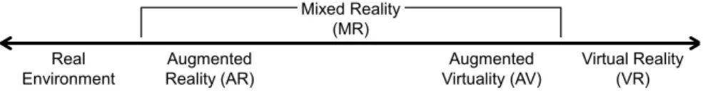
The worlds of the real and the synthetic are colliding more often now than ever before. The year 2016 has seen major consumer releases of several consumer-grade Virtual Reality (VR) headsets (e.g., Oculus Rift CV11, HTC Vive2, and PlayStation VR3), and many other companies are also working on releasing VR headsets of their own. In addition, with the proliferation of smartphones around the world, mobile VR headsets (e.g., Samsung Gear VR4, Google Cardboard5, and Google Daydream6) are also gaining some traction. When users put these these devices on their heads, each of these systems “transport” people elsewhere in the world or into other worlds; however, they also disconnect users from reality by hiding it behind the obscuring goggles. In VR, only virtual objects are visible; the real world need not exist. In Augmented Virtuality (AV), while virtual objects comprise the majority of the combined scene, some real objects are also present.
On the other hand, Augmented Reality (AR)—another form of Mixed Reality (MR) (seeFigure 1.1)— which mixes the virtual world into the real, is beginning to overshadow VR. AR adds virtual objects into the real world. The iOS and Android gamePok´emon Go7has been downloaded over 500 million times by people all around the world (Lynley, 2016). While other games have offered virtual imagery overlaid onto live video of the real world,Pok´emon Gohas been the first to achieve that level of popularity, enabling its users to wander the world while looking through their phone screen and camera to find life-size virtual creatures. Games like these are example uses of Video See-through Augmented Reality (VST-AR) displays, where the
1https://www.oculus.com/rift/
2
https://www.vive.com/
3https://www.playstation.com/en-us/explore/playstation-vr/
4
http://www.samsung.com/global/galaxy/gear-vr/
5
https://vr.google.com/cardboard/
6https://vr.google.com/daydream/
7
Mixed Reality (MR) Real
Environment
Augmented Reality (AR)
Augmented Virtuality (AV)
Virtual Reality (VR)
Figure 1.1: The reality-virtuality continuum, originally proposed by Milgram et al. (1995).
augmenting virtual imagery is overlaid on top of a live, tracked video stream as captured by a camera. The user is no longer looking directly at the world; a display sits in-between and presents both at the same time. This gives the system a great level of control: while the user is free to move, the system can briefly delay the “live” video to allow for processing and rendering time.
Optical See-through Augmented Reality (OST-AR) displays, however, let users continue to look directly at the real world; the virtual imagery is optically combined with the real, which greatly increases the complexity. Optical combination, without any matting, often results in the virtual imagery appearing translucent, but the real world remains visible behind and around the virtual; the disconnect is lesser. The dynamic range (brightness) of the real world also greatly exceeds that of conventional displays. As a result, presenting both worlds with consistent appearance on conventional displays can be impossible in common circumstances. Lastly, and most importantly, with the real world directly visible, even a small amount of time lag (latency) between the user moving and the virtual imagery updating can be visible and highly distracting. Our brains interpret eye-perceived visual displacements differently depending on information from the other senses; when the senses do not agree, we misinterpret the motion (Wallach, 1987). For instance, the appearance of a real object can appear to change in the same way when it is moving and rotating or when the person is moving and rotating, and our vestibular-ocular system distinguishes it based on the other senses. In VR or in AR where the augmentation dominates the user’s view, the user may misperceive the environment as moving when, in fact, only the user’s head is moving and the system was slow to update. A fully effective (and non-distracting) OST-AR display should resolve these issues, among others.
1.2 Motivation
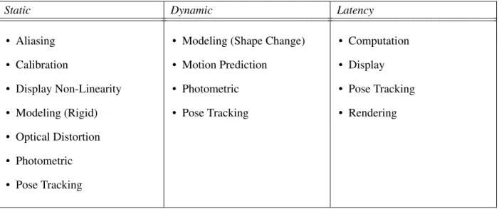
Table 1.1: Example forms of error in AR systems.
Static Dynamic Latency
• Aliasing • Calibration
• Display Non-Linearity • Modeling (Rigid) • Optical Distortion • Photometric • Pose Tracking
• Modeling (Shape Change) • Motion Prediction
• Photometric • Pose Tracking
• Computation • Display • Pose Tracking • Rendering
The work presented in this thesis focuses on subsets of two of the major issues that plague AR displays: latency and the dynamic range of the real world (photometric). Solving these sources of error would greatly improve users’ experiences with these types of displays, so long as the solution for one does not nullify the solution for others.
1.2.1 Latency
Maintaining the illusion of AR requires that the two worlds be registered to each other, spatially and temporally. Of the many types of registration errors existing in AR systems, system latency is the largest, outweighing all others combined (Holloway, 1997; Brooks, 1999). Latency induced errors take many forms, though mostly as “swimming” and “judder.” Both types of errors are highly distracting to many users, and can induce simulator sickness (Pausch et al., 1992) in VR situations.
Latency errors can also result in the virtual imagery appearing to smear and strobe (“judder”). Judder errors result from the discretization of time, typically by the frame rate of the display, but also by the sample rate of slow tracking systems. Both the HTC Vive and the Oculus Rift CV1 use 90 Hz low-persistence displays for VR, which helps; although, for OST-AR, updates at these rates can cause quite visible displacement (see Section 3.1). However, some systems or complicated graphics applications are unable to keep to a 90 Hz schedule and require additional techniques to compensate for the slower render rate, which (without this compensation) would have further increased the latency.
Past approaches to reducing latency have included applying a Post-Rendering Warp (PRW)—i.e., last minute improvements—to the imagery using the latest tracking information (Mark et al., 1997; Smit et al., 2010). In addition, the notion of updating displays in raster order (top-to-bottom, left-to-right) is fading as new display technologies lend themselves to very high frame rate, frameless, or random-order update schemes (Bishop et al., 1994; Dayal et al., 2005). Some of these techniques were originally developed when graphics systems could not keep up with standard 60 Hz displays; now they can be extended to support kHz-order displays, which suffer from the same relative problem.
1.2.2 Dynamic Range
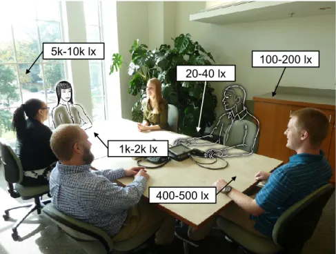
The real world is a High-Dynamic Range (HDR) environment (seeFigure 1.2 for an example). Thus, HDR displays for AR are necessary for the user to comfortably and simultaneously perceive both the real and virtual worlds in close visual proximity. This closeness may be physical (i.e., a tree’s shadow on a bright sunny day) or temporal (i.e., entering or exiting a windowless building). While the human visual system can see both extremes simultaneously, conventional cameras cannot (in a single exposure) capture both. Furthermore, conventional displays (i.e., an 8 bit/color display) lack the necessary range.
5k-10k lx
20-40 lx
100-200 lx
400-500 lx 1k-2k lx
Figure 1.2: A sample scene of people in a room with HDR brightness, captured by a standard camera, annotated with relative brightness measurements from physical points around the scene, and augmented with two simulated people.
1.3 Thesis Statement
In Augmented Reality displays, the combination of performing Post-Rendering Warps in display hardware to mitigate latency registration error and using scene-adaptive, High-Dynamic Range color to improve the consistency of virtual and real imagery decreases the disagreement of the two worlds.
1.4 Contributions
The main contribution of this dissertation is presenting the implementation and design principles of a Head-Mounted Display (HMD) for OST-AR supporting HDR, RGB (Red, Green, and Blue) color. This design offers some characteristics not previously achieved by OST-AR HMDs: an average end-to-end latency of 80 µs for a 6 bit monochrome display and of 126 µs for a 16 bit/color HDR display. These displays use a new low latency rendering approach that breaks the standard display paradigm of sense→render→warp→
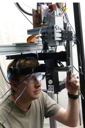
Figure 1.3: A user “wearing” our AR display. The monocular virtual imagery is presented to the user’s left eye.
binary-based displays requires both connecting the tracking system and coupling the latency compensation process directly to the display modulation mechanism. Contributions specific to each of these approaches are listed in Sections 3.1.1 and 4.1.1. An example of the author using an early iteration of the implemented display is presented in Figure 1.3.
1.5 Structure
CHAPTER 2: BACKGROUND
2.1 Introduction
This chapter provides a background into the realm of AR and concepts necessary to understand the work presented in the later chapters. Section 2.2 reviews related work and existing systems in AR and low latency display techniques. Our system uses a Digital Micromirror Display (DMD) (Hornbeck, 1997), which is a type of SLM, at the core of the display; Section 2.3 provides an explanation on how DMDs work. Lastly, Section 2.4 provides background on simple modulation techniques, which can be applied to binary displays, like DMDs.
2.1.1 Units
In the discussion that follows in this document involving multiples of units, SI prefix notation is used: k = 1000, M = 1 000 000,etc. For consistency, SI prefix notation is also used for computer memory sizes of bits (b or bit) and bytes (B): 1 kbit = 1000 bit, 1 Mbit = 1 000 000 bit,etc.
2.2 Related Work
There has been a lot of past and recent work on AR displays and reducing latency for AR, VR, and conventional displays. This section provides background regarding all of the above.
2.2.1 Existing Near-Eye OST-AR Displays
(Maimone, 2015). Nearly all commercial displays provide an FOV (about 40° along the diagonal) much smaller than even eye glasses (≥100°).
Some, like the OST Google Glass1or the VST Vuzix M100 or M300 Smart Glasses2, are marketed as stand-alone devices. They combine an Android™-based smartphone-level System on a Chip (SoC) device with a small display, worn on glasses (or frames). The display, however, is not centered in the user’s vision but is instead offset to the side of one eye’s FOV, leaving a mostly unobstructed view of the real world. These types of systems may not truly be AR, but instead provide a user a smartphone computer experience in constant, hands-free view. They may provide context-sensitive information or a Heads-up Display (HUD), but they are limited in ability for providing an MR experience.
Other systems go for a more mainline AR experience where the virtual imagery is in the center of the view. The Meta 2 Augmented Reality Headset3provides a wide FOV (90° diagonal), OST-AR experience. However, it is a tethered experience; it is connected to a traditional PC. Despite this, backpack PCs—currently being offered to support room-scale VR experiences—could be applied to it as well. On the other hand, systems like HoloLens4or Lumus’ development kits5provide stand-alone OST-AR experiences. The former provides an integrated mini-PC running a special version of Windows®, while the latter runs Android™. Integrated tracking on all of these systems allows the user to turn their head or move around the room while keeping a virtual appearance integrated into the same space, with varying levels of quality.
While these existing OST-AR displays may differ in implementation, part of the display experience, however, is common to all: namely the frame rate and render loop. None of these displays exceed a full-color frame rate of 120 Hz, though some are color sequential at higher speeds (e.g., the HoloLens operates at 60 Hz overall, but each color appears for a fraction of the 1/60 s frame time). While the render loops could support deferred rendering or GPU preemption (seeSection 2.2.4.1) for a last-minute PRW, they remain subject to displaying an image (or a color plane of an image) for a full frame time (or sub-frame time). This would be a best-case latency of 1/120 s for a 120 Hz simultaneous color display (or 1/180 s for a 3-color 60 Hz sequential
1https://www.google.com/glass/start/
2
https://www.vuzix.com/Products
3
https://www.metavision.com/
4https://www.microsoft.com/microsoft-hololens/
5
display), which can produce a noticeable displacement between real-world and virtual object correspondences (i.e., a registration error).
2.2.2 Registration Error
A major failure point for AR systems is registration error: if real and virtual objects are supposed to coexist in the same space, but they do not appear in the correct place, then the illusion is broken. Holloway (1995, 1997) and Livingston and Ai (2008) performed error analyses for AR systems. Sources of error takes many forms: static (e.g., optical distortion, calibration, display non-linearity, aliasing, position tracking, and orientation tracking), dynamic (e.g., position and orientation tracking), and latency. Of all of these, however, the greatest source is latency, outweighing all others combined, even at moderate head movement speeds of 500 mm/s and 50 °/s (Holloway, 1997).
Most of the static errors (i.e., errors occurring while the user or scene is not moving) can be resolved by improving system calibration (i.e., properly measuring the relationships among objects, the display, the user, and the scene). Certain tracking errors (both static and dynamic), however, require the use of a tracking system of sufficient quality for the task, which may or may not yet exist, depending on the task’s scope. Latency induced errors, which usually manifest dynamically, require every component in the system to iterate quickly and report quickly. Care must be taken when developing a system to minimize errors to improve the user’s experience, though latency has often been the hardest to solve. Failure to compensate sufficiently for the overall system latency can lead to simulator sickness in users (Buker et al., 2012).
2.2.3 Latency Requirements
upwards of 437 °/s. This would seem to require0.286°/(437°/s) = 0.654 msof latency to meet the 5 mrad standard. Note, however, that for our approximately 30° FOV (horizontal) prototype display, a 5 mrad error manifests as an error of almost 10 pixels, which is quite noticeable. Thus, the non-noticeable tolerances may be tighter.
When considering more moderate head turns, the latency time tolerances may increase. Jerald and Whitton (2009) and Jerald (2009) performed human latency tolerance measurements with a simulated zero-latency HMD and artificially induced scene-motion. They theorized and demonstrated that zero-latency thresholds are inversely proportional to peak head-yaw acceleration. When measuring oscillating users, they found that for their use cases, the users’ ability to detect any latency ranged from 3.2 ms to 60.5 ms (50 % thresholds ranged from −3.2 ms to 103.2 ms), though their user’s head motion profiles varied and the users had no real-objects to measure latency against. As a result, additional study may be needed to find real-world tolerances in OST-AR.
2.2.4 Latency Mitigation Strategies
There have been many past approaches to reduce the effects of system latency in display systems. Perhaps counter-intuitively, many of them involvedelayingcertain operations until the last possible moment. As long as the user’s motion is detected fast enough with high speed tracking systems (e.g., Oculus VR, 2013) or predicted well enough (e.g., Azuma, 1995; Didier et al., 2005) and displayed just-in-time, then there is an opportunity to keep overall end-to-end latency sufficiently low. Several of the techniques discussed in this section were originally developed when graphics hardware was incapable of reaching the frame rate of displays for the desired scenes (a case which remains valid today for complex scenes in video games). When the rendering system runs slower than the display, this further increases the overall end-to-end latency as old display frames are repeated.
2.2.4.1 GPU Improvements
Recent advents in GPUs have targeted improving latency in desktop monitors and in consumer VR displays. G-SYNC™6by NVIDIA® and FreeSync™7by AMD are methods for dynamically modifying the
6
http://www.geforce.com/hardware/technology/g-sync/technology
7http://www.amd.com/en-us/innovations/software-technologies/technologies-gaming/
refresh rates of monitors. Typically, displays run at a fixed frame rate (e.g., 60 Hz), and GPUs run as fast as possible; this difference can cause tearing of the displayed imagery. Enabling VSYNC (Vertical Sync) prevents the tearing—by locking the GPU’s frame rate to match the monitor’s and by delaying processing of subsequent frames—but it can cause latency and stutter when the amount of rendering computation varies. G-SYNC™ and FreeSync™ each allow the GPU to transmit a variable frame rate stream (up to the maximum supported by the monitor), where each frame is transmitted as soon as it is produced. This eliminates the appearance of the stutter and reduces the latency.
Improvements specifically targeting VR displays tend towards supporting exclusive-mode rendering and GPU preemption. The former excludes the Operating System’s (OS’s) compositing engine from managing VR displays, which could have incurred frame delays, and the latter allows for just-in-time, last-moment operations to occur prior to frame transmission with specific timing guarantees.
2.2.4.2 Frameless Rendering
Typical rendering consists of a series of frames, like a movie film reel, where each frame represents a single instant in (or short duration of) time. Each pixel in a frame corresponds to the same time. Frameless rendering, on the other hand, drops that concept, though there are multiple ways in which the concept of frames is ignored.
Bishop et al. (1994) originally proposed a scheme for frameless rendering to avoid two problems: the latency incurred by double-buffering, and the image tearing incurred by not double-buffering. Instead of producing a stream of raster-order frames, they produce a stream of random-order pixels. In this way, they produced a “crude approximation of motion blur.” While they only simulated the method, this type of system could be implemented on a display supporting random access updates or on a raster-order display where the display process greatly exceeds that of the render process. The idea is that multipledisplay frames are used to generate a coherentperceived (orintegrated) frame. Dayal et al. (2005) extended the idea by adaptively choosing which pixels to update based on knowledge of the scene, increasing visual quality with little increase to the rendering overhead.
advantage of low-persistence, raster-order displays by generating the appropriate color for each pixel based on its location at the time it is emitted onto the GPU-display connection. With a zero-latency implementation, a yawing user, turning at any speed, would see each pixel appears aligned, while an external observer (using a cloned monitor) would see the rendered world as horizontally skewed. Recent implementations of this method include the “Ultra Low Latency Frameless Renderer” ray-casting VR system by Friston et al. (2016), which used a Field-Programmable Gate Array (FPGA) renderer to produce a beam-racing system with a latency of about 1 ms from tracker to pixel emitted on an Oculus DK28.
2.2.4.3 Post-Rendering Warp
Post-Rendering Warp (PRW) is a catchall phrase for methods where a normal rendering algorithm is followed by one or more reprocessing steps that transform (“warp”) the conventional output to produce something new. A typical latency-reduction use for PRWs follows an expensive 3D rendering operation occurring that uses old tracking information with some 2D or 3D transform to shift the perspective to match the latest user pose (So, 1997; Pasman et al., 1999; Itoh et al., 2016). Performing this action both supports low frame rate rendering systems (by providing intermediate frames between full renders) and general rendering systems (by realigning the imagery as late as possible). Implementations of PRWs take many forms.
Image-based Rendering (IBR) is a more general PRW technique where the final operation is an image composition algorithm. Regan and Pose (1994) presented the “Address Recalculation Pipeline” as an IBR method. While traditional rendering directly and wholly renders the entire scene for a given time instant, IBR divides up the 3D rendering process object-by-object into multiple 2D+Depth images. Then, at the last possible moment, it uses the latest tracking information to perform a layered composition of the relevant objects’ images. Some IBR implementations combine these schemes with more conventional rendering pipelines (Kajiya and Torborg, 1996; Walter et al., 1999; Dayal et al., 2005).
Other PRW methods perform more complicated operations. Given a set of reference 2D+Depth frames and the corresponding perspectives, one could generate a novel perspective by selectively compositing those views (McMillan and Bishop, 1995; McMillan, 1997). Mark (1999) took advantage the coherence of motion to produce fast interpolated frames between expensive full renders, and Didier et al. (2005) used a pose predictor to help guide the warp. Others have used multiple PCs or specialized hardware between the PC and
8
display to produce latency mitigated imagery for the display (Smit et al., 2008, 2010). Oculus has integrated PRW into their VR headset’s drivers to help game developers lower the experienced latency when their rendering is too expensive or unstable in frame rate, calling it “Asynchronous Timewarp” (Antonov, 2015). Complications with warping arise when the perspectives contain insufficient information and the new perspective looks into the missing regions. 3D warps of these perspectives tends to create holes in the output imagery as objects become disoccluded. For example, in Figure 1.2, if the view shifted slightly to the left, then the right elbow of the leftmost person should be displayed as it emerges behind her neighbor’s head. Thus, as parts of the scene become “visible” in the new perspective, the renderer needs a hole filling operation (e.g., Mark et al., 1997) to hide the gaps. These methods are never perfect in scenes of overlapping objects, as there will always exist a new perspective where the necessary data is unavailable from the reference perspective(s). Nonetheless, the goal is that any new errors introduced by the algorithm are less disturbing than the latency of the original image or an empty gap in the warped image.
2.2.5 High-Dynamic Range
As previously noted, the real world varies greatly in brightness. The human visual system operates well with color vision (“photopic vision”) between about 0.003 cd/m2and 35 000 cd/m2, but can still see luminances less than 0.001 cd/m2(Daly et al., 2013). Conventional displays, however, are much more limited (e.g., 0.1 cd/m2 to 300 cd/m2). Some displays (e.g., Wetzstein et al., 2010; Mann et al., 2012; Microsoft, 2016) employ darkening materials behind their dim and/or limited range display to reduce the brightness of the real world behind it.
An early implementation of an HDR display used a patterned backlight behind a normal LCD (Liquid Crystal Display) screen, providing a luminance range of 0.1 cd/m2 to 10 000 cd/m2 (Seetzen et al., 2003).
This display used controllable, high-brightness Light-Emitting Diodes (LEDs) in an array behind the LCD screen to provide regional brightness control though with localized high resolution detail. By compensating for the low resolution of the backlight in the LCD, they were able to create a display that was not noticeably perceptually different from a purely high resolution HDR display. Pavlovych and Stuerzlinger (2005) performed a similar operation by backlighting an LCD with a digital projector.
HDR-labeled televisions have emerged: HDR-10 (UHD Alliance, 2016), which supports 10 bit/color; Dolby Vision (Dolby, 2016), which supports 12 bit/color; Hybrid Log-Gamma (Borer and Cotton, 2015), which supports 10 bit/color or 12 bit/color; and Advanced HDR (Technicolor, 2016), which supports 10 bit/color. A new standards war may be brewing, though at least this time the specifications are not incompatible; a display can support multiple standards.
2.3 DMD Operations
One of the most accessible display types for low latency approaches is the DMD (Digital Micromirror Display), manufactured by Texas Instruments (TI) under the brand “Digital Light Projection” (DLP®). Low level control of this fast display type has been demonstrated by numerous groups, including Raskar et al. (1998); McDowall and Bolas (2005); Jones et al. (2009); and Bhakta et al. (2014). Since the presented system makes extensive use of a DMD, it is useful to present how DMDs work. Our system uses the TI DLP® Discovery™ 41009 (Texas Instruments, 2013b), which uses a DLP7000 DMD chip (Texas Instruments, 2013a), which is capable of XGA (Extended Graphics Array) resolution (1024×768). The discussion below uses the specification and parameters of this display in its explanation.
2.3.1 DMD Chip Basics
A DMD chip is essentially a binary-data, double-buffered, Random Access Memory (RAM) device, where one of the buffers represents a 2D array (DLP7000 active diagonal length: 0.7 in) of tiny mirrors (pitch: 13.68 µm). The first buffer (the “back buffer,” in rendering terminology) is user-writable, where each memory entry in the 2D array is one bit. The other buffer’s (the “front buffer”) bits control the pitch of the mirrors, where “0” and “1” correspond to pitches of±12°. The mirrors are binary in nature; a programmer cannot specify any stable in-between angles.
Access to the back buffer is exposed by row addressing; the controlling processor can load any row with a complete row’s worth of data, and then jump to any other row and load it. The DLP7000 supports pixel clocking speeds between 200 MHz and 400 MHz, and each row requires 16 clock cycles to load completely, supplying 64 binary pixels per clock cycle. Rows are grouped into blocks, each of 48 rows, though the writing process can jump among blocks freely.
9
To copy data from the back buffer to the front buffer’s mirrors, the controlling processor must issue a Mirror Clocking Pulse (MCP). On the DLP7000, the processor can issue an MCP at any time between row loads, as long as at least 4.5 µs have passed since the previously issued MCP. When issuing an MCP, the processor can specify that one, two, four, or all of the blocks should be copied from back to front buffers. However, once an MCP has started, the processor cannot make any changes (back or front) to the affected blocks for 12.5 µs, during which the mirrors in those blocks are stabilizing.
The restrictions on loading blocks undergoing MCPs limits the random-access utility of DMDs. At 400 MHz, loading one block requires(16×48)/(400 MHz) = 1.92µs, which is less than the minimum gap between MCPs: 4.5 µs. As a result, using raster scan order (left-to-right, top-to-bottom) and issuing two- or four-block MCPs is much more efficient, resulting in the maximal binary frame rate (32 kHz at 400 MHz).
2.3.2 Conventional DMD Projector Basics
Standard DMD projectors typically spatially illuminate the entire active surface of the DMD uniformly. Controlling the pitch of each mirror’s “0” or “1” values corresponds to deflecting the illumination source either out of the display through the projection lens (“1”) or into a light absorbing baffle (“0”). Producing non-binary grayscale values requires controlling the relative proportion of emitted light for each pixel over time. Generating such analog (grayscale) values from binary values is on form of modulation that is central to later discussion (seeSection 2.4).
DMD projectors typically provide color either by optically combining multiple DMD chips—each with different colored illuminators—or by using color-sequential methods on one chip. In the past, color sequential methods used a spinning color wheel, cycling among red, green, and blue; newer projectors may cycle among colored LEDs, but the basic process is the same. While a single color is active, the DMD undergoes a modulation sequence for that color. For a standard 60 Hz projector, the three colors may alternate at 180 Hz. Some displays may also incorporate white light illumination into the sequence to increase maximum brightness.
schemes of the projectors often require complete frames to start execution, the controlling processor must buffer a complete frame internally before starting to load the DMD’s back buffer, resulting in a display latency of at least one video frame. This delay is unacceptable for low latency OST-AR.
2.4 Modulation
The use of a DMD requires conversion of grayscale pixel values to a sequence of binary frames that approximate those values. This is a form of analog-digital-analog conversion: each “analog” pixel value is represented as annbit grayscale value, which is converted to a series of binary “1” and “0” values that represent white and black projected values, which in turn, due to persistence in the human visual system, the user sees as an analog grayscale value with2npossible levels. Generating analog values from binary values is called modulation. Modulation is extendable to other high speed displays or transmissions that support binary input and need variable output (Jang et al., 2009; Greer et al., 2016).
To display a given 6 bit intensitydover a period of 63 bit-times, the light is turned “on” fordbit-times and “off” for the remaining times. The “on” and “off” pulses are integrated (in this case, by the human eye), and result in the appearance of the desired intensity. The differences between the schemes presented below are in the selection and order of whichdbit-times should be “on”. The selected algorithm affects the perceived quality of the resulting image (e.g., flicker) and determines the requisite hardware resources (memory storage and bandwidth and computation time). As long as the time to execute the sequence of binary frames is short enough, flicker should be minimal. On a DMD, where the illuminator is typically constantly on, the equivalent operation for turning the light “on” and “off” is instead flipping the mirror to the “on” and “off” angles.
To generalize, suppose a modulationm(d, s)exists, wheredis the desired intensity andsis the step index. Most Pulse Train Modulation (PTM) approaches on DMDs require an exponential number of binary frames to execute one full integration cycle:O(2n), wherenis the number of bits in the supported desired value.
g=
2n−1
X
s=0
b×m(d, s) (2.1)
One could extend valuesdandginto functions of pixel coordinates, and then this summation sequence could be applied to DMDs. Furthermore, the value ofdcould change with time, irrespective of the current step within the summation. For notational simplicity, those positional and time variables are suppressed in all examples that follow.
There are two well-known PTM approaches for converting analog signals to bitstreams (i.e., a sequence of binary values): Pulse Width Modulation (PWM) and Pulse Density Modulation (PDM). In both approaches, the pulse generator operates at a high enough frequency so that the moving average closely approximates the analog value, when averaged over a window of time smaller than the human eye’s response time. Some examples of execution sequences of these exponential-time PTM schemes are presented in Figure 2.1.
2.4.1 Pulse Width Modulation
In PWM, the width of the pulse of light generated is varied in direct proportion to the desired gray value at the pixel, as illustrated in Figure 2.1’s left column. Thus, for a given window size, a 25 % gray value will generate a two-part pulse that is “on” for 25 % of the time and “off” for the remaining 75 % of the time window. When considering a discretized window, generating a 6 bit intensity requires 63 steps per interval. Thus, using the notation of Equation (2.1), the summation function for PWM can be as defined in Equation (2.2a), wheremPWMis defined in Equation (2.2b).
gPWM=
2n−2
X
s=0
b×mPWM(d, s) (2.2a)
mPWM(d, s) =
1 ifs < d
0 otherwise
(2.2b)
2.4.2 Pulse Density Modulation
PWM PDM (Delta-Sigma) d = 4 0 0.25 0.5 0.75 1
0 15 30 45
0 0.25 0.5 0.75 1
0 15 30 45
d = 8 0 0.25 0.5 0.75 1
0 15 30 45
0 0.25 0.5 0.75 1
0 15 30 45
d = 10 0 0.25 0.5 0.75 1
0 15 30 45
0 0.25 0.5 0.75 1
0 15 30 45
d = 12 0 0.25 0.5 0.75 1
0 15 30 45
0 0.25 0.5 0.75 1
0 15 30 45
pulses are issued in a repeating pattern, with each pulse a fraction of the integration cycle’s duration. For many intensity values, this pattern can repeat during one integration interval. In effect, PDM is equivalent to a much higher frequency PWM for those values, which results in output that is much smoother in time.
The ideal method for generating PDM pulses is known as Delta-Sigma Modulation (∆Σ) (Aziz et al., 1996), illustrated in Figure 2.1’s right column: an “on” pulse is generated if the accumulation of all the prior “on” pulses (“sigma”) is an entire unit (“delta”) less than the integration of the desired gray value over that time. While Delta-Sigma is a very powerful approach with many variants (e.g., higher-order integrators, continuous-vs. discrete-time,etc.), for the specific case of fixed-rate binary values, it is equivalent to Bresenham’s line drawing algorithm (Bresenham, 1965): an increment inxis accompanied by a change inyonly if the deviation from the desired line would be more than one unit. However, Delta-Sigma implementations impose a significant memory cost: they require at least as much memory as storing one desired image, since an error term must be maintained for each pixel. Using the notation of Equation (2.1), the summation function for Delta-Sigma can be as defined in Equation (2.3a), wherem∆Σis defined in Equation (2.3b);e∆Σ, the error
term, is defined in Equations (2.3c) and (2.3d); anddmax, the maximum supported desired value, is2n−1.
g∆Σ= 2n−2
X
s=0
b×m∆Σ(d, s) (2.3a)
m∆Σ(d, s) =
1 ife∆Σ(d, s)≥dmax−1
0 otherwise
(2.3b)
e∆Σ(d,0) =d (2.3c)
e∆Σ(d, s) =
e∆Σ(d, s−1) +d ife∆Σ(d, s−1)< dmax−1 e∆Σ(d, s−1) +d−dmax otherwise
(2.3d)
Note that subsequent summations in this notation should instead definee∆Σ(d,0)as the last value ofe∆Σin
CHAPTER 3: LOW LATENCY RENDERING
3.1 Introduction
Rendering complex scenes remains a time-intensive task, and the high-throughput render pipelines on modern computers do not always lend themselves to keeping latency low. Recent advances in GPUs, with optimizations for VR, have provided reductions in end-to-end latency (seeSection 2.2.4). Unfortunately, performing all of the latency compensation in the PC, prior to transmission to the display, is insufficient for OST-AR. It may be sufficient for VR because VR has less stringent requirements for latency than OST-AR.
Consider the following example using an OST-AR HMD. Suppose the user’s eye sees a 1080p display with a 60° horizontal FOV using a 60 Hz refresh rate. Suppose also that the user has an accurate zero-latency tracker, and that there is no system latency for processing that tracking data into the GPU’s output. Thus, in this example, the only sources of system latency are for transmission and display. Conventional video transmission methods and displays typically require one frame time (the inverse of the frequency) to handle both steps simultaneously, though some displays, like DMDs, require one frame time for transmission and one more for display. If the user were panning his or her head at a constant 60 °/s, a relatively slow speed for humans, then, over the course of one frame, the world would appear to turn behind the image by 1°, which would be one-sixtieth of the display or 18 pixels (or double for a buffering display, like conventional DMDs). Despite the generous assumptions on the tracker and system, at least an order of magnitude increase in frame rate would be required to keep the frame duration latency error down to less than a pixel at these slow head turn speeds.
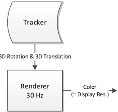
Renderer 30 Hz
3D Rotation & 3D Translation
Tracker
Color (= Display Res.)
Figure 3.1: A sample, conventional render pipeline. Operation rates are given as examples for illustrative purposes only.
processing at very high rates (on the order of 16 kHz). Section 3.2 presents a theoretical solution, while Section 3.3 presents an implementation of a subset of the theoretical solution.
3.1.1 Contributions
• A real-time implementation of a simplified render cascade pipeline, namely the 2D-translation component, in FPGA hardware with an average end-to-end latency of about 80 µs to 126 µs, depending on color depth support.
3.2 Render Cascade Pipeline
As part of a solution towards solving the AR latency problem, consider the following solution as an extension of PRW (seeSection 2.2.4.3): a render cascade pipeline. While PRWs have typically occurred in the GPU at video rates, consider extending a normal render pipeline with distinct stages of warps, where some may occur outside of the GPU (i.e., in the display controller hardware). All stages in this kind of system need not be limited by video rates or external video transmission mechanisms such as VGA, DVI, HDMI, or DP. Each new stage, between a typical 3D render and the final light-emitting display, performs a warping operation to mitigate the latency between the previous stage’s output and the latest tracking information. Later stages could perform simpler actions than prior stages, thus enabling the later stages to execute more frequently.
Tracker 30,000 Hz
Renderer 30 Hz
3D Rotation & 3D Translation
3D Reprojection Warp 300 Hz
Color & Depth (> Display Res.)
2D Warp 3,000 Hz
Color (> Display Res.)
2D Offset 30,000 Hz
Color (> Display Res)
3D Rotation & 3D Translation 2D Rotation & 2D Translation 2D Translation
Color (~ Display Res.)
Radial Distortion Correction 30,000 Hz
Color (= Display Res.)
(a) A sample pipeline with a fast tracker.
Renderer 30 Hz
3D Reprojection Warp 300 Hz
Color & Depth (> Display Res.)
2D Warp 3,000 Hz
Color (> Display Res.)
2D Offset 30,000 Hz
Color (> Display Res)
Color (~ Display Res.)
Tracker
3D Rotation & 3D Translation
Pose Predictor 300 Hz Pose Predictor 3,000 Hz Pose Predictor 30,000 Hz
3D Rotation & 3D Translation
3D Rotation & 3D Translation 2D Rotation & 2D Translation 2D Translation
Radial Distortion Correction
30,000 Hz
Color (= Display Res.)
(b) A sample pipeline with a slow tracker and fast prediction.
Figure 3.2: Two sample PRW pipelines with faster later stages than earlier stages. Operation rates are given as examples for illustrative purposes only.
Consider the notional example in Figure 3.2(a), which depends on a high-frequency, low-latency tracker to supply information to each stage before displaying on a high-frequency display. This example takes a slow 30 Hz renderer and processes the imagery to make it suitable for a 30 kHz display, which is in the typical range for DMDs. As some of these processes (at the declared rates) exceed the current capabilities of GPUs and the bandwidth of current video cable specifications, some of the later steps would need to occur after transmission from the GPU. In the absence of such a high-quality tracker, Figure 3.2(b) presents an alternative where the motion profile of the tracked object is sufficiently characterized to be predicable. Unfortunately, certain stages of motion (e.g., the initial jerk at the start) are difficult to predict, and the results may be worse for it.
While these pipelines attempt to reduce the detectability of latency, in some ways, they also increase it. A normal 30 Hz renderer would typically be ready to output its imagery immediately after each frame, but the animation content of that frame (in this notional system) would be delayed by at least 3.7 ms (1/300 Hz + 1/3000 Hz + 2×1/30 000 Hz), and this assumes instantaneous transference of intermediate frames; a real system would require more time. As long as the delays in a real system would continue to be short enough to maintain each stage’s assumption of small required changes, the final output would be improved (w.r.t.pose) when compared with the typical render pipeline, but certain content would be delayed. For instance, if the internal structure or color of a virtual object changed, that information would be delayed by the pipeline. It remains to be seen by user studies if this would be more distracting, but the swimming resulting from misaligned imagery is already known to be distracting, and the described render cascade pipeline could reduce or perceptibly eliminate this misalignment.
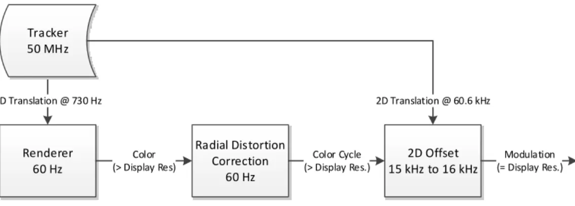
3.3 Prototype: Simplified Render Pipeline
Renderer 60 Hz
2D Translation @ 730 Hz
Radial Distortion Correction
60 Hz
Color Cycle (> Display Res.)
Tracker 50 MHz
Color (> Display Res)
2D Offset 15 kHz to 16 kHz
Modulation (= Display Res.) 2D Translation @ 60.6 kHz
Figure 3.3: The PRW pipeline implemented in our prototype. Operation rates were measured using the constructed prototype.
3.3.1 Components and Implementation
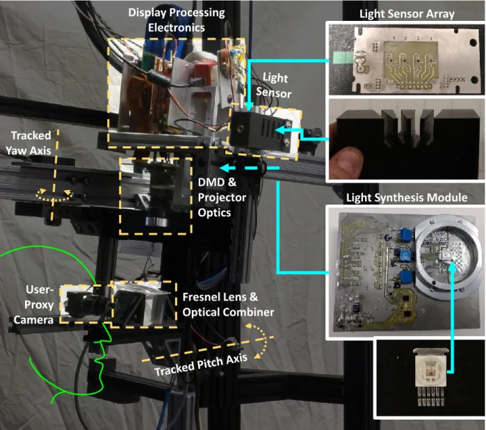
Our prototype hardware setups for an OST-AR HMD using a DMD are presented in Figures 3.4 and 3.5. They employ a combination of traditional PC/GPU rendering with a post-rendering, post-transmission FPGA-based display update process. Virtual elements of the AR scene are rendered on the PC1and transmitted via DP to the display processing system for latency mitigation and emission. That system consists a Xilinx Virtex®-7 FPGA board2interfaced to a TI DLP® Discovery™ 4100 Kit3, which is composed of a Xilinx Virtex®-5 FPGA board4, an XGA DMD module, and projective optics. The DMD is capable of displaying binary frames to the user at up to 32 kHz though our implementation limits it to rates on the order of 15 kHz to 16 kHz. Figures 3.6 and 3.7 present the implemented data paths.
To track the user’s motion, we use high resolution rotary shaft encoders5, each with 40 000 ticks of resolution per revolution (0.0009 °/tick). Using shaft encoders like this limits the HMD to only angular motion. This “open-loop” tracking system, using quadrature encoding, is processed by a Digilent FPGA
1
Our system used an NVIDIA® GeForce® GTX™ Titan Black (http://www.nvidia.com/gtx-700-graphics-cards/ gtx-titan-black/) GPU for rendering.
2Our system used the HTG-777 (http://www.hitechglobal.com/Boards/Virtex-7_FMC.htm), which has an XC7VX690T-2FFG1761 Virtex®-7 chip ( https://www.xilinx.com/products/silicon-devices/fpga/virtex-7.html).
3http://www.ti.com/tool/dlpd4x00kit
4
This board has an XC5VLX50-1FF1153 Virtex®-5 chip (https://www.xilinx.com/support/documentation/ data_sheets/ds100.pdf).
5
Rear projection panel Rear projection panel
Fresnel lens Fresnel lens Camera Camera Projector Projector Visual target Visual target Yaw axis, tracked with shaft encoder Yaw axis, tracked with shaft encoder Camera Camera
Figure 3.4: System assembly for the 6 bit/pixel system. Display electronics include a TI DLP® Discovery™ 4100 Kit, an HTG-777 FPGA board, and a custom DP input and interconnect board. Projector components include the XGA DMD chip and standard lens assembly. The remaining optics include the rear projection panel, Fresnel lens, and beam splitter (half-silvered mirror). Either a user or a camera can observe the optically combined physical and virtual visual targets.
board6. Tracking data is routed both to the render PC and the display processing system using separate high data rate RS-232 serial links. Each device receives tracking updates at a rate in excess of its display update rates.
The PC performs standard AR rendering from the user’s (or test camera’s) tracked and calibrated perspective, with one significant modification. Typically, one would render the scene to produce a 2D image directly suitable for display at the same resolution as the display from that perspective, performing any necessary radial distortion correction as well. In order to supply additional content for the PRW (“2D Offset” in Figure 3.3) renders a larger viewpoint; the display is capable of showing XGA resolution, but our PC renderer produces imagery in 1080p. The output from the GPU is such that the central 1024×768 region of the 1920×1080 output and that the central region is properly corrected for radial distortion. We used OpenCV’s camera calibration library (Bradski, 2000) to perform the viewpoint calibration.
6
Display Processing
Electronics
User-Proxy
Camera
Fresnel Lens &
Optical Combiner
DMD &
Projector
Optics
Tracked
Yaw Axis
Light Sensor Array
Light Synthesis Module
MLX75305 Photosensor Xilinx
Spartan-III FPGA on Digilent Board
Combined
Live Tracking Data Standard RS-232 Bandwidth: 115.2 kbit/s Tracking Rate: 730.5 Hz
PC
2 of
Live Tracking Data RS-232 over Twisted Pair Bandwidth: 2 Mbit/s (each) Tracking Rate: 60.6 kHz (each)
2 of Shaft Encoder
Quadrature Encoding
DisplayPort™ 1.2 Frame Size: 1920×1080×24b
Frame Rate: 60 Hz Embedded Tracking Data
Binary Pixel Data
Data Rate: 128 pixels per clock at 100 MHz Frame Size: 1024×768×1b Maximum Link Frame Rate: 16 kHz
Xilinx Virtex-5 FPGA on TI DLP®
Discovery™ Kit Board
DMD 2 of 2048×1536×6b
Dual-Ported Memory DisplayPort™ Decoder Offset Computation & Windowed
Image Reader Write
P ix el D ata 4 pi xe ls p er v id eo c lo ck F ra m e S iz e: 1920 × 1080 × 6b
Read Pixel Data 128 pixels per 100 MHz clock Frame Window Size: 1024×768×6b DMD Control R ea d A dd re ss es 1 op p er 100 M H z cl oc k
Image Tracking Data 1 pose per frame
− C1 C2 C3 Emitted Light C4
(j) TI OPT101 Photosensor (a) Pitch/Yaw 2-Axis Shaft Encoder Tracking System C1 (b) PC (c) DisplayPort™ Decoder (d) External Triple-Buffered Color Separated DDR3 Memory (f) Internal Double-Buffered Monochromatic Dual-Ported Memory (e) Offset Computation for Display Window
(g) DMD Control
(h) DMD (i) EmittedImage
Live Tracking Data 60.6 kHz
Live Tracking Data 730.5 Hz
1080p (24 bit) Video Stream w/ Embedded Tracking Data
60 Hz
3 × Color Separated 1080p (8 bit) Frame w/ Embedded Tracking Data
60 Hz
Monochromatic 1080p (8 bit) Frame 956 Hz
Monochromatic XGA (8 bit) Frame 15,302 Hz
XGA Window Coordinates
15,302 Hz
Binary XGA Pixels 15,302 Hz
Reflected Image Image Tracking Data
C4 C2
C3
To achieve low end-to-end latency, we divide the rendering pipeline between the PC and FPGA. As a side channel in the GPU rendered image, we embed the then-current tracking information used to render that image. To ensure that the embedded information remain synchronized to the rest of the image, we enabled VSYNC, which prevents prevent tearing, on the GPU. Independently, the display processor (FPGA) receives the live tracking information directly from the tracking system. When it is time to begin displaying a 16 kHz binary frame, it uses both the viewpoint calibration and difference in the two tracking states to transform the latest image to the current viewpoint. Essentially, the display processor is performing a post-rendering (and post-transmission) warp.
To simplify the processing required on the FPGA for this warp, we make some assumptions about the motion. Our tracking system only supports motion along two rotational dimensions (pitch and yaw), and the center of projection of the moving viewpoint is near to those two rotation axes. We also assume that the difference in angular pose between the render-time pose and the live pose is small. Thus we can simplify our warp into a 2D translation and crop of the GPU-supplied imagery; essentially we select a particular 1024×768 window of the full rendered image for each output display frame. As a result, that “excess” resolution provided by the GPU becomes padding for the offset computation engine. For each dimension, the offset from center (∆) of this window in the input frame is simply the product of the difference of the rotation angles (ω) with the ratio of display pixel resolution (r) to field-of-view angle (α), as shown in Equation (3.1).
∆ = (ωlive−ωrender)×(r/α) (3.1)
In the event that the user managed to move faster than the resolution provides, out-of-bounds pixels are replaced by black by the FPGA logic, though we did not encounter this in our live tests.
Depending on the implemented color output of our display system, we used two different memory architectures for storing and processing the GPU-supplied imagery. These are described below.
we had to limit the grayscale resolution to 6 bits/pixel, which we found visually sufficient. By using a double-buffered framebuffer in the FPGA, we are generally able to read from a buffer with a consistent tracking state. It is occasionally possible that the writing process may have switched buffers just after the reading process decided on which buffer to read from, but because the reading process (about 16 kHz) is orders of magnitude faster than the writing process (60 Hz), the discrepancy would last for only a small portion of one binary frame. If we were to use only a single framebuffer, then the tracking state would not be consistent across the whole image while the writer was modifying it, which would affect many binary frames. Using two framebuffers to store the desired imagery keeps the reading algorithm and address offset computation simpler, at the expense of doubling the memory required for storing desired imagery.
16 bit/color High-Dynamic Range Color Implementation Like the grayscale implementation, the Vir-tex®-7 FPGA receives the DP-provided frames at full resolution but instead first stores them in DRAM (Dynamic Random Access Memory) external to the FPGA chip. Each color (red, green, and blue) is stored separately, to optimize reading back of a single color at a time; our display is color-sequential. Each color, in turn, is read back into chip-internal, double-buffered, 2048×1080, 8 bit/pixel, dual-ported SRAM to support another highly parallelized modulation engine (seeSection 4.4). To ensure consistent brightness among color channels, this DRAM-read/SRAM-write process, operating at 956 Hz, is phase-locked to the color sequence. The SRAM read process produces binary frames at 15 302 Hz. The SRAM reading process for producing offset computations is the same as in the grayscale implementation.
3.3.2 Visual Results: 6 bit/pixel Grayscale Implementation
We conducted an experiment to assess the efficacy of our implementation. More specifically, our aim is to determine how well our implementation maintains registration between real and augmented objects as the user turns his or her head.
3.3.2.1 Experimental Setup
(white and dark gray) virtual checkerboard is displayed on the HMD. As the HMD pans, the two should stay locked together. Due to the nature of the checkerboard pattern, any misregistration will be quite obvious.
A GoPro® HERO4 Black camera was mounted in the HMD approximately at the location of a user’s left eye. The camera is rigidly-attached to the HMD rig. The full assembly is shown in Figure 3.4.
For the experiment, the HMD is rotated back-and-forth over a range of about 30°, which is approximately the horizontal field of view of the display. Rotation was performed by hand. To provide consistent angular velocity among trials, we mounted a protractor scale to the top of the HMD and used a metronome to time the back-and-forth movements. The HMD was rotated such that it moved 10 degrees per beat (for three beats) and then rested for one beat. We executed experiments with metronome speeds of 100 and 300 beats per minute. Thus we see consistent acceleration, constant velocity, and deceleration time periods in both directions. The resulting angular velocities equate to approximately 17 °/s and 50 °/s, respectively.
Videos were recorded at 240 Hz both with and without our latency compensation system enabled at each of the two angular velocities; some sample frames are shown in Figure 3.8. Our movement technique allowed for nearly-synchronized side-by-side comparisons of the respective tests. While the camera uses a rolling shutter, the horizontal axis of the image plane and the tested motion patterns were aligned, so comparisons along that axis remain valid.
3.3.2.2 Discussion
Representative samples from the resulting videos under motion are shown in Figure 3.8. Figures 3.8(a) and 3.8(b) depict typical behavior with our latency compensation system disabled. Specifically, the image displayed on the HMD is updated only as new frames arrive from the GPU (at 60 Hz). In Figure 3.8(b), which was the 50 °/s case, we see that the displayed image lags the real-world image by almost three squares. In general, the augmented image lags behind the real-world image by an amount proportional to the rate of movement and the two worlds come into registration onlyafterthe motion ceases. It is worth noting that doubling the GPU frame rate to 120 Hz would not meaningfully mitigate this effect, as the lag would be reduced by at most half of the displacement.
(a) Conventional display method. Panning velocity is approximately 17 °/s.
(b) Conventional display method. Panning velocity is approximately 50 °/s.
(c) Our display algorithm. Panning velocity is approxi-mately 17 °/s.
(d) Our display algorithm. Panning velocity is approxi-mately 50 °/s.
blur in the augmented image is consistent with that of the real-world object. The blur is smooth and natural, significantly due to updating the input to our modulation scheme at a high rate; as the tracking information has the potential to update every binary frame, the window on the desired image can also update. The eye or camera continuously integrates these moving binary frames, resulting in motion blur.
The virtual checkerboard could occasionally become misaligned to its physical counterpart; this typically happened at one end of the motion path. It is worth noting that at those faulty HMD poses, both the conventional display algorithm and our latency compensating algorithm would agree on the amount of misalignment if the HMD were not moving at the time. The source of this unfortunate misalignment was that the rig to which our HMD was mounted allowed for slight freedom of motion along axes that were not tracked, which repeatedly affected the calibration and caused the static divergence between the real and virtual worlds. This highlights the necessity for using high quality and accurate tracking and calibration schemes in order to support AR applications in which the two worlds must be rigidly aligned. It is worth noting that while actively moving, even in the poor calibration zones, our algorithm kept the two worlds closer.
3.3.3 Visual Results: 16 bit/color HDR Implementation
We repeated the checkerboard latency oscillation test from Section 3.3.2.1, though with a larger checker-board (12 cm squares) located about at a distance of 3 m from the display (seeSection 4.4.2 for a longer discussion of the room setup and camera used;seeFigure 3.5 for an image of the system assembly). The HMD was rotated back and forth over a range of approximately 15° by hand at multiple target average velocities: 6 °/s, 12.5 °/s, 25 °/s, and 50 °/s. The movement range was smaller for this system in order to keep the larger checkerboard always inside the display’s FOV. Videos were recorded at 45.45 Hz of both the latency-compensation enabled and disabled situations, and representative frames are shown in Figure 3.9. Results were similar as with the grayscale implementation. Furthermore, no color separation effects, which might be expected from a color sequential display, were visible in the results.
3.3.4 Latency Analysis: 6 bit/pixel Grayscale Implementation