CONSTRUCTING WEIGHTS TO USE IN ANALYZING PAIRS OF INDIVIDUALS FROM ADD HEALTH DATA
Kim Chantala
Carolina Population Center
University of North Carolina at Chapel Hill August 2001
Investigating certain research questions may involve linking the responses of one adolescent to those of another adolescent interviewed in the Add Health Survey. The goal of the analysis will be to characterize the behavior of a pair of adolescents rather
than the behavior of an individual adolescent. Unfortunately, the available sampling
weights are appropriate only when the analysis seeks to investigate behaviors of individual adolescents. However, an appropriate sampling weight can be constructed for each pair of adolescents and used to correct for clustering and unequal probability of selection of the pair. This paper covers the types of pairs of adolescents that can have a pair weight constructed, describes the necessary formulas and data, and concludes with an example showing how to compute pair weights for romantic partners from the Wave II In-home Interview.
Types of Linked Pairs of Adolescents
The most common types of linked pairs in the Add Health data are:
• Friends: Respondents and the friends they listed (available from the In-School, Wave I and Wave II In-home Interviews).
• Couples: Respondents and the romantic partners they listed (available from both the Wave I and Wave II In-home Interviews).
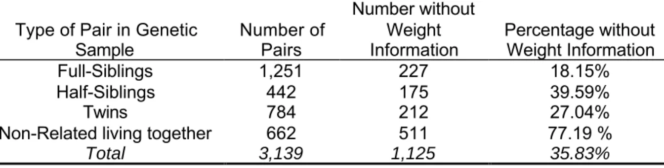
There is no information available to compute sampling weights for pairs of adolescents that are not included in the probability sample. These pairs are additional siblings who did not attend any of the 132 schools selected from the sampling frame and were interviewed to increase the sample size for genetic analysis. The number of pairs of friends or couples that cannot have pair weights computed is small and should not affect having sufficient sample size for analyses. However, 35.83% of the pairs in the genetic sample do not have weight information for both members of the pair (table 1). This is a large enough percentage that you may decide to do your analysis without any correction for unequal probability of selection of genetic pairs. Since your results may not be nationally representative unless you use sampling weights, a thorough
description of the characteristics of the genetic sample would be very helpful to someone wanting to generalize your results to their own group of interest.
Table 1. The percent of pairs that do not have information for constructing pair weights.
Type of Pair in Genetic
Sample Number ofPairs
Number without Weight
Information Percentage withoutWeight Information
Full-Siblings 1,251 227 18.15%
Half-Siblings 442 175 39.59%
Twins 784 212 27.04%
Non-Related living together 662 511 77.19 %
Total 3,139 1,125 35.83%
Probability Sample
Genetic Sample
Linking Data for Pairs of Adolescents
Adolescents were asked to identify their friends and partners using the combined
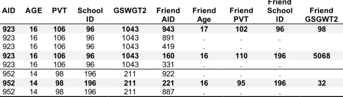
rosters from the high school and feeder school. The Add Health identification number of the friend (or partner) was saved in the data set. To link the records of two adolescents, you will need to merge the data from the respondent with the data collected from their friend (or partner) to create a data set as illustrated in Table 2. The respondent with AID=923 nominated five friends, but only two of the friends were interviewed. Similarly, only one of the friends nominated by AID=952 was interviewed. Only these three of the eight friendship pairs are available to be in the data set used to describe the target population of teenage friends.
Table 2. Example of data representative of Add Health friendship pairs from Wave II.
AID AGE PVT School
ID GSWGT2 FriendAID FriendAge FriendPVT
Friend School
ID GSGWT2Friend
923 16 106 96 1043 943 17 102 96 98
923 16 106 96 1043 891 . . .
923 16 106 96 1043 419 . . .
923 16 106 96 1043 160 16 110 196 5068
923 16 106 96 1043 331 . . .
952 14 98 196 211 922 . . .
952 14 98 196 211 221 16 95 196 32
952 14 98 196 211 887 . . .
Computing Pair Weights
The first step is to compute an initial pair weight. This can produce some pairs of adolescents whose computed weights will be extremely large, thereby increasing the variability of the weights and any estimates computed from them. To minimize the variance and bias of estimates, a trimming procedure is used to limit the value of extreme weights. This is an iterative procedure that allows you to find the optimal value for trimming the weights and construct a desired set of pair weights. To understand the details of this technique, pair weights will be computed for romantic partners from the Wave II In-Home Survey.
Formulas for Pair Weights
There are two basic formulas for computing the initial pair weights. Appendix A shows how the formulas were derived. The only information needed for these formulas is the sampling weight of each adolescent (WEIGHT) and the sampling weight for the school
from which they were sampled (SCHOOLWT). The formula used if the pair of
1) The Pair of Adolescents (i and j) were sampled from the same feeder or high school
(k):
k j i
j i
SCHOOLWT
WEIGHT
WEIGHT
PAIRWT
,=
∗
2) The Pair of Adolescents (i and j) were sampled from a high school and the
associated feeder school:
School High
j i
j i
SCHOOLWT
WEIGHT
WEIGHT
PAIRWT
_ ,
∗
=
The primary sampling unit becomes the High School. This means that to correct for clustering of respondents, the students that were sampled from a feeder school will be assigned to the associated high school.
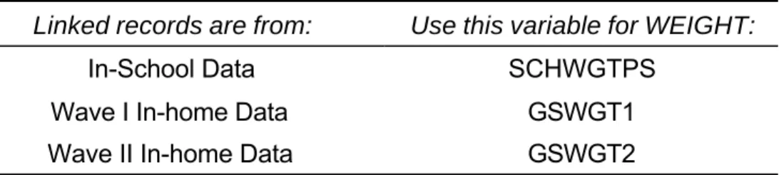
Data Used in the Pair Weight Formulas
Use SCHWT1, the Add Health sampling weight variable for the school attended, in place of SCHOOLWT in the previous two formulas. You may need to request this
variable from the Add Health data manager. The variables you need to use in place of WEIGHTi and WEIGHTj in the previous formulas are the variables for each adolescent’s
sampling weight that you normally use in analysis for individuals. These are listed in Table 3. Notice that you will use the adolescents’ weight variable from the data set you used to link the records.
Table 3. Variable names for an adolescent’s sampling weight in each data set.
Linked records are from: Use this variable for WEIGHT:
In-School Data SCHWGTPS
Wave I In-home Data GSWGT1
Wave II In-home Data GSWGT2
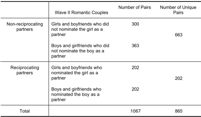
Example 1. In the probability sample, there are 983 adolescents from Wave II who nominated 1067 opposite-sex partners who were also interviewed at Wave II. These relationships can be broken down as shown in Table 4. The couples have been divided into two groups: respondents whose partners also nominated them (reciprocating
partners). While there were 1,067 nominated relationships, there are only 865 unique couples. This is because the 202 boys with their reciprocating partners make up the same couples as the 202 girls with their reciprocating partners.
Table 4. Wave II couples.
Wave II Romantic Couples Number of Pairs Number of UniquePairs
Girls and boyfriends who did not nominate the girl as a partner
300 Non-reciprocating
partners
Boys and girlfriends who did not nominate the boy as a partner
363
663
Girls and boyfriends who nominated the girl as a partner
202 Reciprocating
partners
Boys and girlfriends who nominated the boy as a partner
202
202
Total 1067 865
The task is to use the pair weight formulas to construct sampling weights for the 865 unique couples from the Wave II In-home Survey.
A data set has been constructed linking the identification numbers of the school(s) attended, the schools’ weight, and the grand sample weights from Wave II for the respondent and the partners they nominated. Table 5 shows what the data might look like for three of these couples.
Table 5. Hypothetical data for three couples.
AID SchoolID SCHWT1 GSWGT2 PartnerAID School IDPartner SCHWT1Partner GSGWT2Partner
923 96 68 1043 943 96 68 98
923 96 68 1043 160 196 124 5068
952 196 124 211 221 196 124 32
1,503.15 68
98 1043 923,943
PAIRWT = ∗ =
77,734.18 68
5068 1043
923,160
PAIRWT = ∗ =
54.45 124
32 211 952,221
PAIRWT = ∗ =
All three pairs would be assigned to the primary sampling unit (PSU) corresponding to school 96 (the high school). Notice that the large individual weights for PAIRWT923,160
have created a very large pair weight.
Using these same formulas, initial pair weights have been computed for the 865 unique couples from Wave II. Here are the descriptive statistics for these initial pair weights computed using PROC UNIVARIATE in SAS:
UNIVARIATE STATISTICS ON INITIAL PAIR WEIGHTS
N 865 Mean 10933.56 Std Dev 30393.84 Variance 9.2379E8 Sum 9457532
PERCENTILE VALUES
100% Max 672945.8 75% Q3 9507.123 50% Med 3378.266 25% Q1 700.0378 0% Min 20.06924
99% 110294.9 95% 47011.17 90% 28557.53 10% 159.5563 5% 84.89495 1% 40.42081
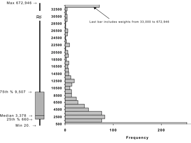
means that our sample represents an estimated 9,457,532 teenage couples from the U.S. The average pair weight is 10,933 and the median value is 3,378. This indicates an extremely skewed distribution, as shown in Figure 2.
Figure 2. Box plot and frequency chart showing the distribution of initial pair weights.
The box-plot at the left of the figure shows the range and quartiles of the distribution. From this diagram it is easy to see than most of the pair weight values are small: 25% are below 660 and 50% are below 3,378. The interquartile range contains all the values between the 25th (value of 660) and the 75th percentile (value of 9,507).
The top bar shows there are 71 initial pair weights with values between 33,000 and 672,946. All the other bars are in increments of 1,000.
0 100 200
500 2500 4500 6500 8500 10500 12500 14500 16500 18500 20500 22500 24500 26500 28500 30500 32500
Frequency 25th % 660→
Max 672,946 →
Min 20. →
75th % 9,507 →
Median 3,378 →
Procedure for Trimming the Initial Pair Weights
This section gives an overview of a procedure that can be used to find a set of adjusted weights that minimizes both the variance and the bias in estimates (Potter, 1990 and Potter, 1993). The details of how to perform each step will be illustrated using the couples initial pair weights computed in the previous example. This procedure can be broken down into the following steps.
1. Select a set of values based on percentile cut-points of the initial pair weights that will be used to trim the weights. For example, you may select the values from the 80th percentile to the 99th percentile. Each value will be used to create a set of
adjusted weights.
2. Using each cut-point, truncate the initial pair weights at the cut-point and redistribute the excess sample weight uniformly over all pairs below the cut-point to create a set of adjusted weights. The excess sample weight is the difference between the sum
of the untrimmed weights and the sum of the trimmed weights. To redistribute the excess weight uniformly, divide the excess weight by the number of untrimmed weights, and add this value to the initial weights below the cut-point.
3. Select a set of Add Health data items to use in evaluating which set of adjusted weights is the best to use.
4. Using each set of adjusted weights, compute the Mean Square Error (MSE) for each data item as follows:
BIAS = ESTIMATEInitial Wt – ESTIMATEAdjusted Wt
MSE = VarianceAdjusted Wt + BIAS2
The estimate can be a mean, a proportion, or a regression parameter. 5. For each selected data item, rank the MSEs across all adjusted weights.
6. For each set of adjusted weights, compute the average of the ranks. Choose the set of adjusted weights with the smallest value of average rank MSE to use in
subsequent analyses.
The wisdom of choosing the smallest rank of the MSE will become clear in the example that follows.
Example 2. Use the trimming procedure to determine a set of adjusted pair weights that will give minimum bias and variance for estimates.
Step 1. Choose values for trimming the initial weights. We will need to choose enough
initial pair weight distributions as cut-points for trimming. Table 6 shows these values as computed using PROC UNIVARIATE in SAS.
Table 6. Percentile cut-points for trimming Initial pair weights for Wave II couples. Percent Cut-point Percent Cut-point Percent Cut-point
70% 7,134.34 80% 12,638.35 90% 28,557.53
71% 7,475.42 81% 13,614.24 91% 31,107.67
72% 7,941.88 82% 14,622.08 92% 33,257.42
73% 8,470.67 83% 15,423.71 93% 37,879.85
74% 9,100.29 84% 16,718.79 94% 43,522.64
75% 9,507.12 85% 17,973.99 95% 47,011.17
76% 10,526.52 86% 19,914.61 96% 53,162.82
77% 11,421.12 87% 21,736.53 97% 67,640.99
78% 11,978.12 88% 22,914.57 98% 76,869.29
79% 12,198.29 89% 25,804.63 99% 110,294.94
Here we see that 99% of the pair weights are below 110,295; 85% are below 17,974; and 70 percent are below 7,134.
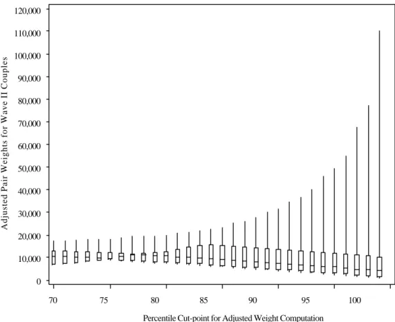
Step 2. Compute a set of adjusted weights for each of the 30 cut-points in Table 6.
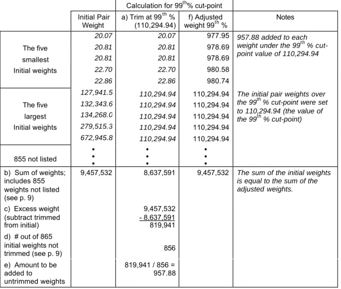
Show the calculations for the five smallest and five largest initial pair weights using the 99th percentile cut-point.
The entries in Table 7 show this calculation for the couples with the five smallest and five largest initial pair weight values. The calculations for the other 855 (see p. 10) unique couples are not listed in the table, but the values for these couples have been included in the computations in row b through row e.
a) Set all initial weights over the value of the 99% cut-point to the corresponding value of 110,294.94 (Table 7, column a).
b) Sum the initial weights and trimmed weights (row b).
c) Determine the excess weight by subtracting the sum of the trimmed weights from the sum of the initial weights (row c).
d) Determine how many of the initial weights did not need to be trimmed (row d). e) Compute the amount that needs to be added (row e) to each of the untrimmed
weights by dividing the excess weight computed in row c by the number of initial weights that did not need to be trimmed listed in row d.
The sum of the initial weights is equal to the sum of the adjusted weights. This means that the average weight does not depend on the trimming level and remains at
10,933.56.
Table 7. Calculation the set of adjusted pair weights trimmed at the 99th% cut-point
using procedure on page 9.
Calculation for 99th% cut-point Initial Pair
Weight a) Trim at 99
th %
(110,294.94) weight 99f) Adjustedth % Notes
20.07 20.07 977.95
The five 20.81 20.81 978.69
smallest 20.81 20.81 978.69
Initial weights 22.70 22.70 980.58 22.86 22.86 980.74
957.88 added to each weight under the 99th % cut-point value of 110,294.94
127,941.5 110,294.94 110,294.94
The five 132,343.6 110,294.94 110,294.94
largest 134,268.0 110,294.94 110,294.94
Initial weights 279,515.3 110,294.94 110,294.94 672,945.8 110,294.94 110,294.94
The initial pair weights over the 99th % cut-point were set to 110,294.94 (the value of the 99th % cut-point)
855 not listed
• • • • • • • • •
b) Sum of weights; includes 855 weights not listed (see p. 9)
9,457,532 8,637,591 9,457,532 The sum of the initial weights is equal to the sum of the adjusted weights.
c) Excess weight (subtract trimmed from initial)
9,457,532 - 8,637,591 819,941 d) # out of 865
initial weights not
trimmed (see p. 9) 856
e) Amount to be added to
untrimmed weights
819,941 / 856 = 957.88
Step 3. Select several Add Health variables to use in evaluating the adjusted weights.
The choice of data items should represent the possible relationships between the weights and the data expected in the full set of data items. It is important to choose a set of variables where most of the continuous variables do not have values of zero, because a value of zero may mask the influence of an extreme weight (Potter, 1990, page 225). Some variables should also be related to the weights because a negative correlation between the weights and the data can imply that the variation in the weight is good (reduces the sampling variance). However, your data may not be correlated with the weights if the sampling design did not have much over-or under-sampling of
populations. For the Add Health data, we will select both continuous and binary variables. For continuous variables we will want to estimate the mean value and for binary variables we will estimate proportions.
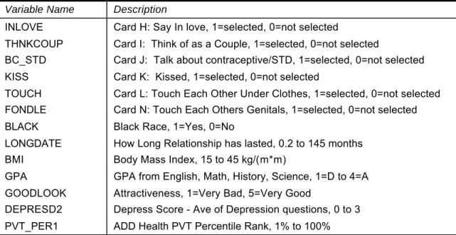
Table 8 shows the variables that were selected. The first six variables are from the section of the Wave II questionnaire that asked respondents to select events in their relationship from a set of cards. These are binary variables with a value of 1 indicating
70 75 80 85 90 95 100
Percentile Cut-point for Adjusted Weight Computation 120,000
110,000
100,000
90,000
80,000
70,000
60,000
50,000
40,000
30,000
20,000
10,000
0
Adjusted Pair Weights for Wave II Couples
there was no association between the initial pair weights for respondents who selected the card versus those that did not select the card. The binary variable BLACK showed a strong association with the initial pair weights. The last six are continuous variables constructed from various Add Health data items. Pearson correlation coefficients indicated only a small association between the sampling weights and these variables and ranged from -0.04 to 0.05.
Table 8. Variables selected to use in evaluating the adjusted weights.
Variable Name Description
INLOVE Card H: Say In love, 1=selected, 0=not selected
THNKCOUP Card I: Think of as a Couple, 1=selected, 0=not selected
BC_STD Card J: Talk about contraceptive/STD, 1=selected, 0=not selected KISS Card K: Kissed, 1=selected, 0=not selected
TOUCH Card L: Touch Each Other Under Clothes, 1=selected, 0=not selected FONDLE Card N: Touch Each Others Genitals, 1=selected, 0=not selected BLACK Black Race, 1=Yes, 0=No
LONGDATE How Long Relationship has lasted, 0.2 to 145 months BMI Body Mass Index, 15 to 45 kg/(m*m)
GPA GPA from English, Math, History, Science, 1=D to 4=A GOODLOOK Attractiveness, 1=Very Bad, 5=Very Good
DEPRESD2 Depress Score - Ave of Depression questions, 0 to 3 PVT_PER1 ADD Health PVT Percentile Rank, 1% to 100%
The data items we have chosen are available for each individual. Since each person in a reciprocated partnership reported the relationship, each can be included in this
procedure to find the optimal set of adjusted weights. Hence, we will use the response from each adolescent reporting the relationship for the 1,067 couples for the
computations in the remaining steps.
Steps 4-5.Use each set of adjusted weights to compute and rank the MSE for each
selected variable.
The computation will be shown for the BMI (Body Mass Index) variable using the adjusted weight computed at the 85th % trim level. Using a package designed for
survey data analysis with the initial pair weight as our sampling weight gives an
estimate of 22.388 as the mean value of BMI. Using the adjusted weight computed at the 85th % trim level gives an estimated mean of 22.605 and standard error of 0.17105
The bias is:
BIAS = 22.388 - 22.605 = -0.217
The mean square error can then be computed as:
MSE = VARIANCE + BIAS2 = (STD ERR)2 + BIAS2
= (0.17105)2 + (-0.217)2
= 0. 0.076 (step 4).
Using BMI, repeat this computation for each set of adjusted weights. The results are displayed in the second column of Table 9.
Examining the formula for MSE shows why it is a good criterion to use in evaluating the effect of the adjusted pair weight. The MSE is composed of two elements crucial to testing any hypothesis: the BIAS and the VARIANCE. A small BIAS indicates our estimate is “close” to the true value. A small variance guarantees that in repeated sampling a higher fraction of our estimates will be “close” to the true value of what we are trying to measure. This means that the smaller the variance the more certain we are that we have estimated the true value and have more evidence from our data to support our hypothesis. We can select the optimal set of adjusted weights for each variable by finding the set that gives us the smallest MSE for all of the data items. The next step is to rank the values of MSE across all of the adjusted weights as shown in the third column of Table 9. The smallest MSE computed used the adjusted weight for the 81st % cut-point (assigned a rank of 1) and the largest MSE was computed using
the adjusted weight for the 98th % cut-point (assigned a rank of 30). The value we
Table 9. MSE computed using each of the adjusted weights and rank of MSE for BMI.
Adjusted Weight at cut-point Step 6) MSE for BMI Step 7) Rank of MSE
70 0.0896 22
71 0.0872 19
72 0.0890 21
73 0.0846 18
74 0.0822 17
75 0.0800 13
76 0.0795 12
77 0.0807 14
78 0.0770 7
79 0.0717 2
80 0.0748 4
81 0.0717 1 ←smallest
82 0.0787 11
83 0.0776 9
84 0.0815 16
85 0.0761 6 ← example
86 0.0783 10
87 0.0774 8
88 0.0729 3
89 0.0760 5
90 0.0814 15
91 0.0879 20
92 0.0914 23
93 0.0923 24
94 0.0948 27
95 0.0946 26
96 0.0955 28
97 0.0973 29
98 0.0982 30 ← largest
99 0.0940 25
Step 6. Average the ranks of the variables for each of the adjusted weights.
The ranks for all of our seleted variables are listed in Table 10. The last column is the average of the ranks for each row and can be used to compare the overall effect of each of the 30 adjusted weights. Examining this column shows that the smallest average rank is for the set of adjusted weights at the 85th % cut-point. This is the set
that can be used in any analyses on romantic pairs from Wave II.
Table 10. Ranks for MSE computed using all 30 adjusted weights for each variable.
Ranking of MSE values Adjusted
weight cut-point
BC_STD BLACK BMI DEPRESD2FONDLE GOODLOOKGPA INLOVE KISS LONGDATE PVT_PER1THNKCOUP TOUCH RankAve.
70 24 30 22 20 20 30 30 1 22 29 30 23 21 23.23
71 28 29 19 22 14 29 29 2 27 28 29 22 19 22.84
72 30 28 21 26 6 28 28 3 29 25 28 20 18 22.31
73 29 26 18 24 4 27 27 4 30 23 27 21 17 21.31
74 26 27 17 27 5 26 26 5 26 13 26 19 15 19.85
75 27 25 13 25 2 24 25 6 28 12 25 17 14 18.69
76 25 24 12 28 1 25 24 7 24 15 23 12 10 17.69
77 23 23 14 29 3 23 23 13 25 16 24 14 3 17.92
78 22 22 7 30 15 22 22 9 20 9 21 9 5 16.38
79 20 21 2 23 12 21 21 14 21 8 22 11 2 15.23
80 21 20 4 21 13 20 20 12 23 7 20 8 1 14.62
81 18 19 1 19 19 19 19 8 19 4 19 6 9 13.76
82 17 18 11 18 18 17 18 10 16 3 18 3 8 13.46
83 13 17 9 17 16 16 17 11 18 2 17 4 6 12.54
84 10 16 16 15 11 18 16 15 17 5 16 1 4 12.31
85 8 15 6 12 9 15 15 16 14 6 15 2 7 10.77
86 6 14 10 11 8 14 14 18 13 24 14 5 11 12.46
87 4 13 8 14 10 13 13 23 12 22 13 7 13 12.69
88 7 12 3 16 7 12 12 26 11 21 12 10 12 12.38
89 2 11 5 13 17 11 11 24 10 18 11 13 16 12.46
90 3 10 15 10 21 7 10 21 9 17 10 15 20 12.92
91 1 9 20 9 22 6 9 19 7 14 9 16 22 12.54
92 5 8 23 8 23 4 8 17 5 11 8 18 23 12.38
93 9 7 24 7 24 2 7 22 4 19 7 24 24 13.85
94 11 6 27 6 25 1 6 25 3 27 6 25 25 14.85
95 12 5 26 5 26 3 5 28 2 30 4 26 26 15.23
96 14 4 28 4 27 5 4 27 1 26 5 27 27 15.31
97 16 3 29 3 28 8 3 30 6 20 3 28 28 15.76
98 15 2 30 2 29 9 2 29 8 10 2 29 29 15.08
Table 11 shows the changes in the estimates for the 13 selected data items when computed with the initial weights versus the optimal adjusted weights trimmed at the 85th % cut-point. The proportion of couples reporting “in love” changed from 0.55 to
0.63 and the length of time dating changed from eight to nine months. The largest percent change occurred in the proportion of black adolescents reporting relationships. The estimate computed with the adjusted weight, 0.16, matches the population estimate of black adolescents computed with the full Wave II In-home sample. All other changes were very small.
Table 11. Estimates from initial weights compared to estimated from adjusted weight at the 85th % cut-point.
Variable Name Estimate fromInitial Weight
Estimate from Adjusted Weight at
85th% Cut-point Difference inEstimates Percent Change inEstimate
BC_STD 0.31 0.32 -0.02 -4.93
BLACK 0.10 0.16 -0.06 -38.58
BMI 22.39 22.60 -0.22 -0.96
DEPRESD2 0.54 0.56 -0.02 -3.91
FONDLE 0.52 0.50 0.02 3.99
GOODLOOK 3.59 3.69 -0.11 -2.93
GPA 2.97 2.88 0.09 2.99
INLOVE 0.55 0.63 -0.08 -11.97
KISS 0.82 0.84 -0.02 -2.47
LONGDATE 8.00 9.28 -1.28 -13.75
PVT_PER1 58.55 57.04 1.51 2.65
THNKCOUP 0.78 0.79 -0.01 -1.37
TOUCH 0.56 0.55 0.01 1.49
The improvement in the design effect (DEFF) is shown in Table 12 for the thirteen data items used to evaluate the adjusted weights. The DEFF is a ratio of the variance
obtained under our complex survey design compared to the variance that would have been obtained if the data had been collected through simple random sampling. The DEFF from the initial pair weights averages 11.8 and ranges from 3.5 to 20.7. Using the adjusted weights at the 85th % cut-point reduced the average DEFF to 3.5 with the range going from 1.0 to 13.9. Two data items (GPA and BLACK) had an increase in DEFF. By computing the ratio of the values in the two DEFF columns, we can see how much larger the variance is if the initial pair weights are used. In general, the improvement in variance is substantial. The variance of estimates from nine of the thirteen data items computed with the initial weights would be over twice as large as the variance of estimates computed with the adjusted weight at the 85th %. The variance
Table 12. Comparison of design effect for estimates computed from initial pair weights to adjusted weights at 85th % cut-point.
Variable Name DEFFInitial =
DEFF from Initial Weight
DEFFAdjusted =
DEFF from Adjusted
Weight at 85th% Cut-point DEFFInitial/ DEFF
Adjusted-BC_STD 5.1 1.8 2.8
BLACK 11.8 13.9 0.8
BMI 8.3 2.1 4.0
DEPRESD2 4.4 2.8 1.6
FONDLE 16.6 2.1 7.8
GOODLOOK 17.2 3.1 5.5
GPA 3.5 4.8 0.7
INLOVE 20.7 1.0 21.3
KISS 13.0 1.7 7.8
LONGDATE 7.9 1.7 4.7
PVT_PER1 10.0 8.1 1.2
THNKCOUP 19.2 1.1 17.3
TOUCH 15.3 1.5 10.3
Effects of Using the Best Adjusted Weight vs. the Initial Weight
To understand how the sampling weight can affect the results, we will compare the proportion of respondents who reported sexual relations for reciprocating versus non-reciprocating partners. The proportions have been reported separately for girls and boys in table 13. The standard errors are larger when the initial weight is used in the analysis. Using the initial weight finds no difference in proportions for girls having reciprocating versus non-reciprocating partners (p=0.12) while the adjusted weights reject the hypothesis of no difference (p≤0.01).
Table 13. Proportion of boys and girls reporting sexual relations with partner, by reciprocating partner status.
Respondent Group Initial Weight*
Adjusted weight at 85th % cut-point* Boys Non-Reciprocating Girlfriend
Reciprocating Girlfriend
Difference in proportions t-test for no difference
0.25 (0.043) 0.61 (0.121)
0.36 (0.130) t=2.78, p≤0.01
0.28 (0.030) 0.47 (0.046)
0.19 (0.052) t=3.71, p≤0.01 Girls Non-Reciprocating Boyfriend
Reciprocating Boyfriend
Difference in proportions t-test for no difference
0.17 (0.041) 0.37 (0.120)
0.20 (0.130) t=1.58, p=0.12
0.22 (0.028) 0.48 (0.043)
For boys with reciprocating partners, a higher proportion are estimated to have had sexual relations with their partner when computed with the initial weights (0.61) rather than with the adjusted weights (0.47). Conversely, a lower proportion of girls with reciprocating partner are estimated to have had sexual relations with their partners when computed with the initial weights (0.37) versus the adjusted weights (0.48). Since the boys with reciprocating girlfriend are the same couples as the girls with reciprocating boyfriends, these proportions are comparing the responses from the male partner to those from the female partner. Hence, we would expect these proportions to be approximately the same as suggested by the estimates computed with the set of adjusted weights at the 85th % cut-point.
Discussion
Adjusting the weights has been shown to reduce the variance and give a more
believable estimate for the example in the previous section. This best adjusted set of weights has been constructed for doing a global analysis on the 865 relationships reported. Analyses can also be done on several sub-populations, such as the 202 reciprocating partners, the 502 girls and boyfriends, as well as the 565 boys and girlfriends.
If the researcher had indicated that the analysis of a certain group was more important than global analysis, more emphasis might have been placed on finding the optimal set of weights for this group. For example, there may be little interest in analyzing the 202 reciprocating partners. In this case, the 502 girls and their boyfriends might always be analyzed separately from the 565 boys and their girlfriends. In this case, an optimal set of adjusted weights could be found for girls and boyfriends and the process repeated for boys and girlfriends. This was done for the Wave II couples and the optimal set of pair weights was still found to be that adjusted at the 85th % cut-point for both of these
Appendix A. Derivation of Pair Weight Formulas
This appendix shows the derivation of the formulas used to calculate pair weights.
Available Data
School Weights
For each school in the probability sample we know the final school weight, SCHWT1. For high schools this weight is the inverse of the probability of selecting the high school:
SCHWT1 = [Pr{high school}] -1
For feeder schools it is the inverse of the joint probability of selecting the feeder school and high school:
SCHWT1 = [Pr{feeder school, high school}] -1
Adolescent Weights
Sampling weights are available for everyone in the probability sample for the various panels of data:
PANEL OF
DATA WEIGHT MEANING
In-School SCHWGTPS Final In-school Weight
Wave I GSWGT1 Final Grand Sample Weight for Wave I participants Wave II GSWGT2 Final Grand Sample Weight for Wave II participants
Assume the probability of selecting one adolescent in the pair is not influenced by the selection of the other adolescent.
For adolescents from a high school (including high schools with an 8th grade) the weight
represents the inverse of the joint probability of selecting the student and selecting the high school:
WEIGHT = [Pr{student, high school}] -1
WEIGHT = [Pr{student, feeder school, high school}] -1
Note that GSWGT1 for Wave I was computed as the average of a set of weights. The set of weights for each adolescent was computed from the different samples for which the adolescent was eligible.
COMPUTATION OF PAIR WEIGHTS
Students from the Same School
The weight for any pair of adolescents is the inverse of the probability of selecting both adolescents and their schools into the sample. For two adolescents denoted by i and j from the same school k:
Pr {kidi, kidj, schoolk} = Pr{ kidi | schoolk}∗ Pr{ kidj | schoolk}∗Pr{schoolk} (1)
By assuming the joint probability of selecting the kid and the school can be represented by:
WEIGHT-1=Pr{kid,school} = Pr{kid | school}∗Pr{school}
Pr{kid | school} = [WEIGHT∗ Pr{school}]-1
and substituting the result into equation 1 gives:
Pr {kidi, kidj, schoolk} = [WEIGHTi∗ Pr{schoolk}] -1∗ [WEIGHTj∗ Pr{schoolk}] -1∗Pr{schoolk}
= [WEIGHTi∗WEIGHTj∗ Pr{schoolk}] -1
= SCHWT1k∗ [WEIGHTi∗WEIGHTj] -1
So the pair weight for two students from the same school will be:
PAIRWTi,j = WEIGHTi∗WEIGHTj /SCHWT1k (2)
Students from High School and Associated Feeder School
Pr {kidf, kidh, schoolf , schoolh}
= Pr{schoolf , schoolh} ∗ Pr{kidf | schoolf} ∗ Pr{kidh | schoolh} (3)
The first term following the equality sign is the joint probability of both the feeder and high school combination and is multiplied by the product of the conditional probability that each adolescent was selected given that his or her school was selected.
Note for kids from feeder schools:
WEIGHT f –1 = Pr{ kidf, schoolf, schoolh } = Pr{ kidf | schoolf }∗Pr{ schoolf ,schoolh }
So Pr {kidf, kidh, schoolf , schoolh} =
Pr{ schoolf, schoolh} ∗ [WEIGHTf∗ Pr{schoolf , schoolh}]-1∗ [WEIGHTh∗ Pr{schoolh}]-1
= [ WEIGHTf∗ WEIGHTh∗ Pr{schoolh }]-1
= [ WEIGHTf∗ WEIGHTh]-1∗SCHWT1h
The pair weight for a pair composed of a student from the feeder school and a student from the high school is:
PAIRWTf,h = WEIGHTf∗WEIGHTh /SCHWT1h (4)
References
Potter, Frank J. “A Study of Procedures to Identify and trim Extreme Sampling Weights”, 1990, ASA Proceedings of the Section on Survey Research Methods, American
Statistical Association (Alexandria, VA), pages 225-230.
Potter, Frank J., “The Effect of Weight Trimming on Nonlinear Survey Estimates”, 1993, ASA Proceedings on the section on Survey Research methods, American Statistical Association (Alexandria, VA), pages 758-763.
SAS Institute., SAS/STAT User’s Guide, Version 6, Fourth Edition, Volumes 1 and 2, Cary, NC: SAS Institute Inc., 1989