Determining Optimal Number of Suppliers in a Multiple Sourcing Model under Stochastic Lead Times

Vol. 2, No. 1, pp 16-27 Spring 2008

Determining Optimal Number of Suppliers in a Multiple Sourcing Model

under Stochastic Lead Times

Mohammad Reza Akbari Jokar1*, Mohsen Sheikh Sajadieh2

1 _{Department of Industrial Engineering, Sharif University of Technology, Tehran, Iran} [email protected]

2 _{Department of Industrial Engineering, Sharif University of Technology, Tehran, Iran} [email protected]

ABSTRACT

Employing more than one supplier and splitting orders between them is a strategy employed in supply chains to lessen the lead-time risk in unstable environments. In this paper we present a multiple-sourcing inventory system with stochastic lead-times and constant demand controlled by a continuous review, reorder point-order quantity inventory policy. We consider the situation in which the order quantity is equally split between a number of identical suppliers. The aims of this research are to determine the optimal number of suppliers and analyze the percentage savings obtained in a multiple-sourcing system compared to sole-sourcing. The objective function is to minimize the expected total cost per unit time by obtaining the number of suppliers, the reorder point and order quantity as decision variables. Extensive numerical examples are used to examine the effects of different parameters on the percentage savings and the optimal number of suppliers.

Keywords:Multiple-sourcing, Lead-time risk pooling, Stochastic lead times

1. INTRODUCTON

In single sourcing inventory models, when an order is placed with a vendor, it is assumed that the whole order quantity is received in a single delivery from the supplier in each order cycle. It is also possible that the orders can be placed with multiple suppliers so that portions of the order quantity arrive at different times. When the replenishment order quantity is split into several portions, one for each supplier, the effective lead time will be the minimum of a set of random variables representing the lead times of all suppliers. In spite of the trend toward the consolidation of suppliers proposed by the just-in-time philosophy, the decision of employing a single or multiple sourcing is still an important issue especially in the situations in which no reliable supplier exists. In other words, employment of more suppliers may be worthwhile due to the reduction in total system cost where split orders are placed simultaneously, assuming uncertain supply lead times. Lower prices, improved quality, a reduction in lead times uncertainty and therefore savings in inventory holding and shortage costs are some of the advantages of order splitting approach.

* _{Corresponding Author}

One of the earliest papers in dual sourcing is attributed to Sculli and Wu (1981). They studied a two supplier inventory system, where supply lead times are normally distributed with different parameters. Using numerical experiments, they showed that dual sourcing can reduce the mean and variance of the effective lead time. Ramasesh et al. (1991) considered a continuous review inventory model in a dual sourcing setting. They used both uniform and exponential lead-times, and analyzed the associated costs and benefits, assuming that the lead times were identical. They considered the reorder point and order quantity as decision variables to minimize the expected total cost per unit time. Ramasesh et al. (1993) extended that work by relaxing the assumption of identical lead time distributions, unit supply price and split proportion.

Hong and Hayya (1992) developed a non-linear programming model to minimize ordering and inventory holding costs subject to quality level and purchase price constraints where total requirements are split among several different suppliers. Lau and Zhao (1993) considered a dual-sourcing model assuming demand or lead times to be stochastic. They indicated that the inventory cost reduction is more affected by savings in cycle stock holding costs than the savings in safety stock holding costs.

Chiang and Benton (1994) investigated the cost functions of sole-sourcing versus dual-sourcing under the normally distributed demand and shifted exponential lead times assumptions. They demonstrated that dual-sourcing performs better than sole-sourcing except for the cases where the ordering cost is high, the lead-time variability is low, or the customer service level is low. Hill (1996) used a comparable framework for cycle stock in analyzing order splitting and showed that multiple sourcing reduces the average stock levels under any generic lead-time distribution.

Sedarage et al. (1999) developed a general multiple-supplier inventory system where lead times of suppliers and demand arrivals are random. They developed a continuous review inventory model where lead times may have different distributions and purchasing prices from suppliers may be different. One of their findings was that placing an order to a supplier with higher lead time mean and standard deviation and with worse purchase price may be economical. Chiang (2001) analyzed splitting an order into multiple deliveries in a periodic review inventory system. It was concluded that the possibility of the multiple-delivery arrangement in the sole-sourcing environment can reduce the average cycle stock and thus the total cost, especially if the cost of dispatching an order is considerable.

Ryu and Lee (2003) considered dual-sourcing models with stochastic lead times and constant demand in which lead times are reduced at a cost that can be viewed as an investment. They used expediting cost functions as an investment to reduce lead times and compared the expected total cost for two models and demonstrated that the model with reduction results in significant savings. Dullaert et al. (2005) studied a dual-sourcing model for determining the optimal mix of transport alternatives to minimize total logistics costs. They assumed a limited number of transportation modes and developed a genetic algorithm to find the optimal solution.

To the best of our knowledge and based the reviews of papers related to order splitting by Thomas and Tyworth (2006) and Minner (2003), except for Sedarage et al. (1999) no work has been done on multiple-sourcing where the total system cost is sought to be minimized. However, the generality of the model considered by Sedarage et al. (1999) made them use some approximations in the total cost and therefore they concluded that the optimal number of suppliers obtained by their model may not be truly optimal. In this research, we relax their approximations for a special case of multiple-sourcing where identical suppliers with exponential lead times are considered. In our model, the probability density functions of net stocks are used to obtain the cost functions. Thus, the optimum

solution is truly optimal. Additionally, in order to obtain the expected inventory and shortage costs, rather than considering all combinations of orders arrivals, a new method is developed. The method lets us easily calculate the cost functions for any number of suppliers. Moreover, unlike with most of previous studies, the model is not limited to the situation in which the on-hand inventory level just after the last delivery exceeds the reorder level.

The rest of paper is organized as follows. In section 2, we discuss the modeling assumptions and notations and also calculate the expected cost functions. Section 3 deals with numerical results and parametric analysis. Finally, we summarize our findings in section 4.

2. MODELFORMULATION

In this study, a model of multiple-sourcing is developed (see Figure 1). The purpose of the model is to minimize the expected total cost per unit time by determining the number of suppliers, reorder point and the order quantity as decision variables. The total cost consists of three elements: ordering cost, inventory holding cost and shortage cost. As some previous studies have considered (e.g. Chiang (2001)), an additive model of ordering cost is applied, where the ordering cost consists of fixed elements including preparing specifications, requesting for and evaluating bids and … (C₁), and variable elements including shipping, handling and inspection cost per delivery (C₂) that increase by the number of suppliers.

2.1.Notations and Assumptions

The following notations and assumptions are used throughout this paper to develop the proposed models.

Notations

n: Number of suppliers D: Demand per unit time Q: Order quantity s: Reorder point

i

L′: The lead time of ith supplier

i

L : The ith order statistic of lead times

λ: Lead time parameter

Figure 1. Two echelon multiple-sourcing supply chain 1

n

D n

Q

n Q

n Q

T: Cycle time

h: Inventory holding cost per unit per unit time

π: Shortage cost per unit per unit time

Assumptions

1. A multiple-sourcing inventory system is considered. 2. The demand rate is deterministic and constant.

3. The acquisition lead time from each supplier is stochastic and follows an exponential

distribution.

4. Lead times are independent and identically distributed.

5. Inventory is continuously reviewed. The orders are placed simultaneously when the inventory

position reaches the reorder level.

6. The order quantity is split equally between suppliers.

7. Shortages are allowed and completely backordered.

8. Time horizon is infinite.

In most of earlier research efforts (e.g. Ryu and Lee (2003)) it has been assumed that the last installation stock goes above the reorder point and thus a renewable cycle is formed to let the authors generalize the calculation of one cycle to the entire time. In this research, we have satisfied the formation of renewal process by a more realistic assumption that is low probability of order crossover. In other words, we assume that the net stock just after the last delivery can be under the reorder point but the orders are received in the same sequence that they are placed, i.e. the last delivery of each cycle will be delivered sooner than the first delivery of the next. Taking order crossover into account makes the model intractable and thus we assume that its probability is negligible.

2.2.Inventory Holding Cost

Considering the time to receive the first supply and the time between the first and the second supply as two random variables in a dual sourcing model, Ramasesh et al. (1991) obtained expected inventory holding and shortage costs for all possible ranges of these variables. Using this technique, they calculate the expected inventory carried and shortage incurred for 10 distinct combinations that cover the possible cases. Based on this method, the cost functions should be obtained for more than 30 combinations if n=3. The increase in the number of combination makes the model intractable and thus a new method needs to be developed for multiple sourcing. Here we develop a new approach which lets us obtain the cost functions for any number of suppliers. In this method, each cycle time is divided ton+1time ranges based on the time of supply arrivals. Since then, the expected inventory holding and shortage cost is obtained for these time ranges.

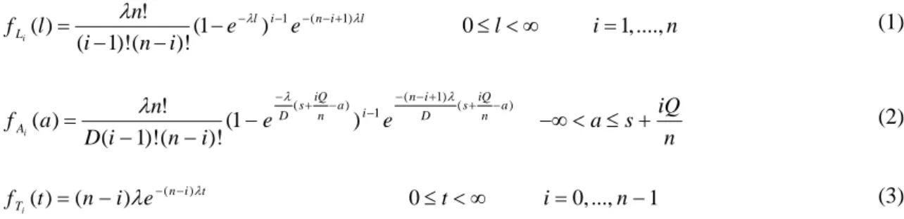
In order to derive expressions for the expected inventory carried during each cycle time, we need the probability density function of the ith order statistic of lead times. We also define two new

random variables A_i =s+iQ n−DL_iandT_i=L_i+1−L_i, which are the net stock just after the ith delivery and the time between ith and (i+1)th delivery, respectively. Net stock is defined as the subtraction of backorders from on-hand stock. Also T₀and T_n have been defined as the lead time of first delivery and the time lag from the last delivery to the end of cycle time. When the distribution of lead times is exponential with parameterλ, the probability density functions ofL_i, A_iandT_i can be obtained as follows using elementary statistics:

n i l e e i n i n l

fLi (1 l)i n i l 0 1,....,

)! ( )! 1 ( ! )

( − 1 ( 1) ≤ <∞ =

− −

= λ −λ − − −+ λ ₍₁₎

n iQ s a e e i n i D n a

f n a

iQ s D i n i a n iQ s D

Ai = − − − −∞< ≤ +

− + + − − − − + − ) ( ) 1 ( 1 ) ( ) 1 ( )! ( )! 1 ( ! ) ( λ λ

λ ₍₂₎

1 ..., , 0 0 ) ( )

(t = n−i e−( −) ≤t<∞ i= n− fTi n i t

λ

λ (3)

As mentioned before, each cycle time can be divided ton+1 time ranges: from the time at which the order is placed to the first delivery, from ith to (i+1)th delivery (for i=1,...,n−1) and from the last delivery to the end of cycle time. The expected inventory carried during the ith time range (I_i) can be obtained, based on the cases that occur during that time range. Two cases can occur during the first time range (Figure 2) depending on the first delivery time.

The expected inventory carried in case 1.1 (EI_1.1) and case 1.2 (EI_1.2) are as follows:

D s n D s n D s l n D s

l L _De

s e n D n s dl e n l Dl s dl l f l Dl s EI λ λ λ λ λ

λ − −

= − = = + − − − = − =

_∫

_∫

l L _De

s dl l f D s EI λ − ∞ = = =

∫

Thus, the expected inventory carried during the first time range (I₁) can be obtained as follows:

) 1 ( 2 2 2 . 1 1 . 1

1= + = + −

− D s n e n D n s EI EI I λ λ

λ (4)

s s

Case 1.1 Case 1.2

0

T T₀

Figure 2. Net stock in the first time range

Time Time

Based on the net stock after ith delivery and the time between ith and (i+1)th delivery, three cases can occur during the (i+1)th time range (Figure 3).

1 ..., , 1 )

( ) ( 2 )

( ) ( ) 2 (

0

2

0 0

2

1=

∫ ∫

∫ ∫

+ =

∞ = +

= =

+ f t f adtda i n

D a da

dt a f t f Dt at

I n

iQ s a

D A

t T A

n iQ s a

D A

t T A

i i i i

i

i i

(5)

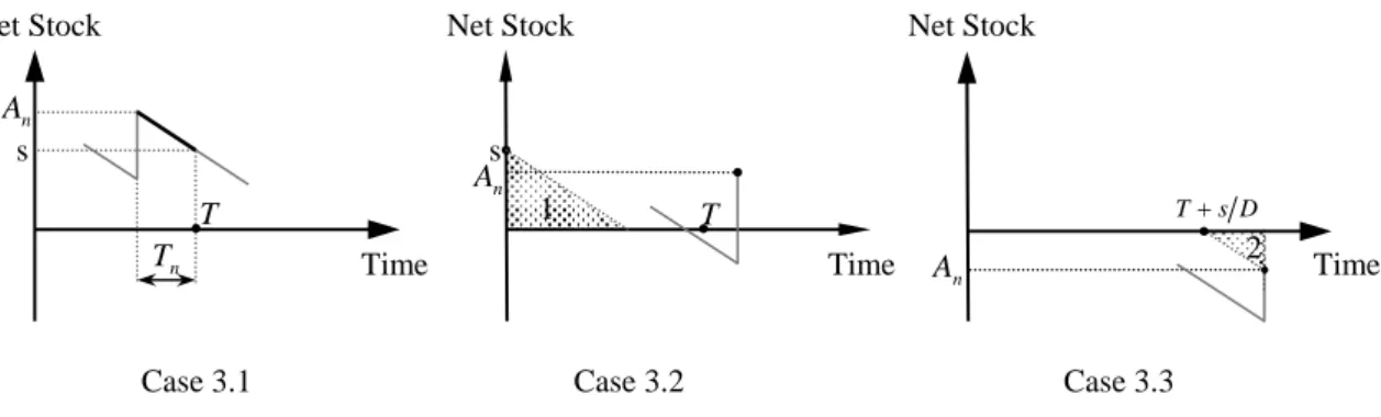
The above expressions can not be simplified before knowing the value of n. Three cases can occur during the last time range (Figure 4) depending on the net stock after the last delivery.

The time horizon of the model is assumed to be infinite. Therefore, as in most inventory systems, we need to obtain the expected total cost for one cycle and then find the expected total cost per unit time. An implicit assumption of this method is that the selected cycle time is a renewable process. If we assume that the on-hand inventory level just after the last delivery is above the reorder point (e.g. Sedarage et al, 1999), thus the start point and finish point of each cycle will be the same (equal to the reorder point) and therefore, the cycle time is renewable. However, in this paper we are not limited to this restrictive situation (case 3.1 in subsection 2.1). Therefore, other situations (case 3.2 and case 3.3) may also occur where the on hand inventory just after the last delivery is not above the reorder point.

The expected inventory carried in case 3.1 where the net stock just after the last delivery is above the reorder point can be obtained easily. However, in cases 3.2 and 3.3, calculation of cost functions needs more discussion. In these cases, the last delivery is received after the cycle time since then the

Case 2.1 Case 2.2 Case 2.3

Time Time Time

Figure 3. Net stock in the (i+1)th time range i

T T_i T_i

i A

i A i

A Net Stock

Net Stock Net Stock

Case 3.1 Case 3.2

Time Time Time

Figure 4. Net stock in the last time range n

A

n A

n A n

T

s s

2 T

1 T+sD

Case 3.3 T

last time range is equal to zero. Nevertheless, in these cases we expand our calculation from cycle time to the time in which the net stock reaches zero (T+s D). The orders to both suppliers are simultaneously placed when the summation of net-stock and ordered quantity, i.e. inventory position, reaches the reorder level. Moreover, as it can be seen in obtaining cost functions in the first time range, the net stock at the start time of each cycle time has been considered to be equal to reorder level, which in cases 3.2 and 3.3 will not be satisfied for next cycle. Thus, assuming no order crossover, we omit the first hatched triangle from inventory holding costs and the second hatched triangle from shortage costs because they will be considered in the next cycle time on average. Not doing this correction makes us calculate the inventory and shortage costs at the same time (shortage for one cycle and inventory for the next or previous one). In other words, in these cases calculation of hatched triangles is shifted to the next cycle. Thus the expected inventory carried in cases 3.2 and 3.3 (EI_3.2 andEI_3.3) will be negative. The expected inventory carried for three cases in this time range is as follow:

∫

−

= s Q

s

a _D fA a da

s a EI

n( )

) 2 ( 2 2 1 . 3

∫

a _D fA a da

s a EI n 0 2 2 2 .

3 ) ( )

2 (

∫

−

= 0 2

3 .

3 ( )

2

a _D fA a da

s EI

n

Thus, the expected inventory carried during last time range (I_n+1) can be obtained as follows:

D s da a f a D EI EI EI

I sQ

a A n n 2 ) ( 2 1 2 0 2 3 . 3 2 . 3 1 . 3

1= + + =

∫

+ =

+ (6)

2.3.Shortage Cost

Employing the same method, the expected shortage incurred during the ith time range (S_i) can be obtained as follows:

D s n e n D S λ λ − = _{2 2}

1 (7) 1 ..., , 1 ) ( ) ( 2 2 ) ( ) ( 2 ) ( 0 0 2 0 2

1 = −

− + − =

_{∫ ∫}

_{∫ ∫}

+ f t f a dtda i n

at Dt da dt a f t f D a Dt S

a t T A

n iQ s a D A

t T A

i i i i i i

(8)

∫

+ =−

0 ₂

1 ( )

2 1

a A

n a f a da

D S

n

(9)

∑

∑

= +

=

+ 1

1 1

1 n

i i n

i

i S

I

h π .

2.4.Expected Total Cost

Using above expressions and resorting to simplification, we get the following expected total cost per unit time (ETCUT):

1 1

1 2

1 1

1 1

2 2 1 2

2 2

2 2 2 2

( )

( )

( 1)

n n

i i

i i

n n

n s n s i i

i i

D D

D

ETCUT C nC h I S

Q

Dh I D S D C nC

Dh s hD D

e e

Qn n Q n Q Q

λ λ

π

π π

λ λ λ

+ +

= =

+ +

− −

= =

= + + +

+ + + = + − + +

∑

∑

∑

∑

3. COMPUTATIONALRESULTS

We need numerical research procedures to find the optimal solution because no closed-form solution exists for the values of s, Q and n that minimize the expected total cost. There is some widely used optimization software to solve the above nonlinear mixed integer programming model.

By substituting the values of integer variable (n) in the model, the problem becomes a pure

nonlinear programming. Therefore, for sensible number of suppliers (n≤10), at most ten pure

nonlinear problems should be solved. Here, the optimal solution is found using LINGO 9.0.

As an example, we obtain optimal solutions for multiple-supplier system for different numbers of

suppliers using the following parameters: D=10000 units/unit time, λ=15 /unit time,

h=$1/unit/unit time, π=$15/unit/unit time, C₁=$120/order and C₂=$30/order. The minimum cost (ETCUT =2028.97) can be achieved by employing four suppliers and ordering a quantity of 814.78 to each one per period, when the net stock reaches 37.4.

We survey the effects of lead time variability, shortage-to-inventory ratio, ratio of fixed-to-variable ordering elements and demand on the optimal number of suppliers. Moreover, the trend of savings percentages obtained by employing more suppliers will be discussed. For these purposes different sets of parameters have been defined: (1) seven levels for the shortage-to-inventory ratio:

] 30 ,..., 10 , 5 , 1 [ /h∈

π ; (2) six levels for the ratio of fixed-to-variable elements of ordering cost:

] 6 ..., , 2 , 1 [ / 2 1 C ∈

C ; (3) eight levels for demand:D∈[2000,4000,...,16000]; (4) twelve levels for lead

times uncertainty: λ∈[10,15,...,65]. The probability of order crossover is less then 0.024 for all cases which is negligible.

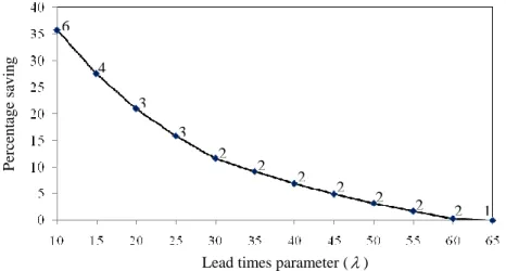
3.1 Different Levels of Lead Time Deviation

As it can be seen in Figure 5, the percentage savings obtained in a multiple sourcing system tends to be higher when lead times are more unpredictable. Moreover, the optimal number of suppliers (the

integer printed above each node in Figure 5) is a non-increasing function ofλ. For instance,

increase in lead time standard deviation from 0.05 to 0.10 changes the optimal number of suppliers from 3 to 6 and percentage savings of employing multiple sourcing from 20.95 to 35.74. The reason is that by increasing lead time variation, the backorder cost increases and therefore lead time

reduction will be more attractive. It also can be interpreted that dual-sourcing is the optimal solution for a wide range of lead time parameters.

3.2 Different Levels of Ratio of Fixed-to-Variable Ordering Elements

We obtained optimal solutions for decision variables in a multiple sourcing inventory system using six different levels of C₁/C₂ whereC1 is assumed to be fixed. We present the results in Table 1. For

the range of parameters used, the percentage savings from multiple sourcing compared to sole-sourcing and number of suppliers increase by the ratio. Although, the improvement in percentage savings has a diminishing rate.

Table 1: Effect of C₁/C₂ ratio on the optimal number of suppliers

Parameters Multiple sourcing

2 1/C

C s Q ETCUT Optimal n Savings (%)

1 221.4 3649.1 2783.9 2 11.26

2 86.9 3457.2 2344.1 3 19.71

3 24.5 3355.1 2149.9 4 24.33

4 37.4 3259.1 2029.0 4 27.56

5 0.0 3214.9 1949.0 5 29.79

6 5.7 3168.3 1886.3 5 31.64

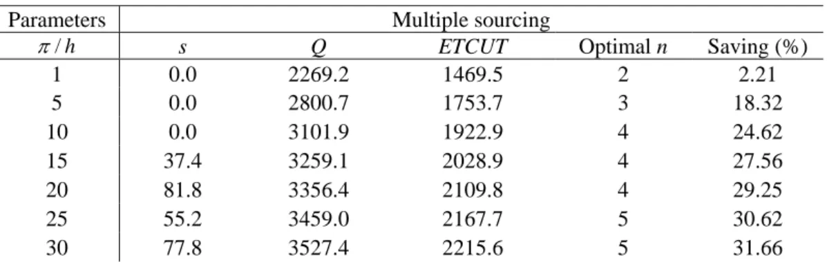
3.3 Different Levels of Shortage-to-Inventory Ratio

The optimal number of suppliers and the percentage savings from multiple sourcing compared to sole sourcing increases by π/h ratio. As mentioned before, increasing the number of suppliers decreases the effective lead time and then the expected inventory carried and shortage incurred. Higher shortage cost per unit per unit time raises the role of shortage cost in the expected total cost and thus more savings can be obtained by reducing the expected shortage incurred. Since then, adding one more supplier may result to savings that outweighs the increased part of ordering cost (see Table 2).

6 4

3 3

2 2

2 2

2 ₂

2 1 Lead times parameter (λ)

Percent

age savin

g

Table 2: Effect of π/h ratio on the optimal number of suppliers

Parameters Multiple sourcing

h /

π s Q ETCUT Optimal n Saving (%)

1 0.0 2269.2 1469.5 2 2.21

5 0.0 2800.7 1753.7 3 18.32

10 0.0 3101.9 1922.9 4 24.62 15 37.4 3259.1 2028.9 4 27.56 20 81.8 3356.4 2109.8 4 29.25 25 55.2 3459.0 2167.7 5 30.62 30 77.8 3527.4 2215.6 5 31.66

3.4 Different Levels of Demand

Figure 6 depicts the trends of savings percentage and optimal number of suppliers for different demand values. A number of facts can be discerned from the figure. First, the percentage savings from multiple-sourcing compared to sole-sourcing increases by demand for a fixed number of suppliers. The main reason is that by increasing demand per unit time, the savings in inventory and shortage costs increase and thus multiple sourcing will be more beneficial. However, most of benefits are recognized by the early increase in demand. Further increase, for all the observed cases, yields only marginal improvements. For example an increase in demand from 2000 to 4000 in a three-supplier system results in 9% increase in the percentage savings while the same increase from 14000 to 16000 results in just 0.64% additional improvement.

Second, the optimal number of suppliers, shown by arrows in Figure 5, increases by demand. This is because inventory and shortage reduction in a system with higher demand may outweigh an additional ordering cost and thus more suppliers may find this beneficial. And third, although increasing the number of suppliers from 1 to the optimal number of suppliers for a fixed amount of demand is beneficial, this improvement is of diminishing kind, with most of benefits realized with the initial increase in the number of suppliers from one to two. This seems to suggest that only limited suppliers should be pursued. This is because most of savings in the inventory holding and shortage costs are obtained by just adding the second supplier and therefore further increases in the number of suppliers will be less effective in improving inventory level and backorder. Thus, in a multiple-sourcing supply chain usually employing two supplier consequences most of benefit of order splitting, except in erratic environments.

4. CONCLUSION

We developed a multiple-sourcing inventory system with stochastic lead times and constant demand where the order quantity is equally split between some identical suppliers. In this paper we employed a new method that lets us obtain the cost functions for any number of suppliers. In this method we divide each cycle to some ranges instead of calculating cost functions for all possible combinations of supply arrivals. Moreover, the model developed in this paper is not limited to the situation in which the last installation stock goes above the reorder point.

Numerical results show that the optimal number of suppliers and the percentage savings from multiple sourcing tend to be higher for uncertain situations with more variable lead times or competitive environments where shortage cost is higher. In other words, as lead time variability increases, the savings from multiple sourcing will also increase and employing more suppliers may be beneficial. Moreover, increase in the factors such as demand and shortage-to-inventory ratio raises the role of inventory carried and shortage incurred in the model, and thus employing more than one supplier as a solution to lessen them will be more motivating.

Furthermore, we found that although increasing the number of suppliers may be beneficial; this improvement is of diminishing kind, with most of benefits achieved by the initial increase of suppliers to two. Therefore, in a multiple-sourcing supply chain employing two suppliers usually leads to the major benefits of order splitting. Thus if it is difficult or costly to obtain the exact number of suppliers, one may consider dual-sourcing as a moderate solution.

Some extensions of this research might be of interest. In this paper, we assumed suppliers to be identical. In practice, they may be different in terms of purchasing price, product quality or delivery time. Moreover, in our current analysis we assumed the costs associated with transportation are part of ordering cost. However, one may consider economies of scale in transportation. Additionally, lead-times are considered to be independent of order quantity. In practice, lead times may be negatively correlated to order quantity.

REFERENCES

[1] Chiang C. (2001), Order splitting under periodic review inventory system; International Journal of Production Economics 70; 67–76.

[2] Chiang, C., Benton, W.C. (1994), Sole sourcing versus dual sourcing under stochastic demands and lead times; Naval Research Logistics 41; 609–624.

[3] Dullaert W., Maes B., Vernimmen B., Witlox F. (2005), An evolutionary algorithm for order splitting with multiple transport alternatives; Expert Systems with Applications 28; 201–208.

[4] Hill R.M. (1996), Order splitting in continuous review (Q,r) inventory models; European Journal of Operational Research 95; 53–61.

[5] Hong J.D., Hayya J.C. (1992), Just-in-time purchasing: single or multiple sourcing?; International Journal of Production Economics 27; 175–181.

[6] Lau H.S., Zhao L.G. (1993), Optimal ordering policies with two suppliers when lead times and demands are all stochastic; European Journal of Operational Research 68 (1); 120–133.

[7] Minner S. (2003), Multiple-supplier inventory models in supply chain management: a review; International Journal of Production Economics 81–82; 265–279.

[8] Ramasesh R.V., Ord, J.K., Hayya J.C., Pan A. (1991), Sole versus dual sourcing in stochastic lead-times, (s,Q) inventory models; Management Science 37 (4); 428–443.

[9] Ramasesh R.V., Ord, J.K., Hayya, J.C. (1993), Note: dual sourcing with non-identical suppliers; Naval Research Logistics 40; 279–288.

[10] Ryu S.W., Lee K.K. (2003), A stochastic inventory model of dual sourced supply chain with lead-time reduction; International Journal of Production Economics 81–82; 513–524.

[11] Sculli D., Wu S.Y. (1981), Stock control with two suppliers and normal lead times; Journal of the Operational Research Society 32 (11); 1003–1009.

[12] Sedarage D., Fujiwara O., Luong H.T. (1999), Determining optimal order splitting and reorder levels for n-supplier inventory systems; European Journal of Operational Research 116; 389–404.

[13] Thomas D.J., Tyworth J.E. (2006), Pooling lead-time risk by order splitting: A critical review; Transportation Research Part E 42; 245–257.

[14] Tyworth J.E., Ruiz-Torres A. (2000), Transportation’s role in the sole versus dual-sourcing decisions; International Journal of Physical Distribution and Logistics Management 30 (2); 128–144.