TRANS_Final_Burton_Allen.pdf

(1)

DETERMINANTS OF CYCLING TO WORK

IN INNER LONDON

by

ALLEN ANTHONY BURTON

A Master’s Project submitted to the faculty of the University of North Carolina at Chapel Hill

in partial fulfillment of the requirements for the degree of Master of City and Regional Planning

in the Department of City and Regional Planning.

Chapel Hill, NC

2014

Approved by:

______________________

(2)

2

Executive Summary

Cycling to work in London, as in many large cities in the Western world, has become increasingly popular in recent years. In fact, the number of journeys by bicycle in Greater

London increased 80 percent from 2002 to 2012 according to Transport for London (TfL, 2013). As London has yet to aggressively expand its on-street bicycle facilities, the trend presents questions about why the growth has occurred. In addition, 2011 UK census data reveals

bicycling has emerged as a much more popular form of transportation in certain parts of London than in others.

The purpose of this paper is to examine what accounts for the spatial patterns of Inner London districts with high rates of cycling to work, using 2011 UK census data on a variety of variables

that have been shown to influence cycling in other research. This study differs from previous studies in London in the extent of variables examined, the geography studied, and in utilization of the recently available 2011 UK census data.

What are the determinants of cycling to work in Inner London?

Through an OLS regression analysis, this study considered a variety of determinants of cycling shown to influence cycling in previous studies. These include

demographic, socioeconomic, and some environmental variables. The study area is Inner London, a geographically

contiguous and relative small area, with a relatively consistent built environment. The geographic unit of analysis is MSOA, a census statistical area with a median population of about 8,000. After adjusting for multicollinearity between variables, outlying observations, and insignificant predictors, the study identified the following as significant variables in predicting the proportion of residents within Inner London MSOAs who cycle to work (the dependent variable), with the direction of association of each indicated in parentheses:

Figure A: Inner London MSOAs by proportion cycling to work in 2011

(3)

3

• Creative workers (+) • 3+ Deprivations (+) • V. Good Health (+) • Male (-)

• White (+)

• Other Households (+) • No car (+)

• Tube station (-) • Transit share (-)

The reduced model containing these variables has an adjusted R-square value of 0.81. The biggest story presented by the findings is the strength of correlation between the dependent variable and the proportion of creative workers in an MSOA (visualized by Figures A and B). Certain findings were surprising in that they ran counter to what would have been expected given past research. These were the negative association between the percent of males in an MSOA and the percent of workers cycling, an insignificant relationship between the existence of bike share in an MSOA and the percent of workers cycling, and also an insignificant relationship between the dependent variable and the percent of young adults in an area.

The results provide a better understanding of the characteristics of Inner London districts with high cycling levels, which is especially pertinent as the city prepares to implement its recently announced “Vision for Cycling in London.” Of particular relevance are the following:

• The findings on creative workers, racial significance, indicate the degree to which

cultural and social influences may be at play in determining the decision to cycle. While some past research has explored this association, it is limited.

• Findings on negative association between the share of workers using transit and the

presence of tube stations suggests a supplementary relationship between cycling and transit in London. This is useful information for transportation planners looking at the transportation network holistically.

The findings also leave many unanswered questions for future research to explore. First and foremost is the question of whether creative workers themselves are cycling more, or there is simply something about the areas they tend to live that are more conducive to cycling. That districts with more men cycle less also leaves unanswered questions, as other studies in London have found men there cycle more. Assessing whether the study’s findings hold for Outer

London, and whether they hold when cycling infrastructure is accounted for would also be of interest for future study.

(4)

4

Acknowledgements

I first would like to thank my advisor, Daniel Rodriguez, for providing thorough and valuable guidance on how to enhance and improve this paper.

I also would like to thank DCRP PhD students Gwen Kash, Lindsay Maurer and Louis Merlin for providing useful feedback when I presented my paper to them.

(5)

5

Bicycle use has increased dramatically in many metropolitan areas in recent years, especially in the Western world. Miles cycled in the UK increased 20 percent from 1998 to 2012 (DfT, 2014), the number of bike commuters in the US rose 64 percent from 1990 to 2009 and by 42% in Canada (Pucher and Buehler, 2011), and by 25 percent in a sample of Danish, Dutch and German cities from 1975 to 1995 (Pucher and Buehler, 2008). Cycling is associated with

improved health (Wen and Rissel, 2007; Pucher et al, 2010), and is an essentially carbon neutral form of transportation in a world becoming more concerned about greenhouse gases and air quality. As a result, many cities are implementing policies to encourage more cycling. London is an example, as Mayor Boris Johnson launched the city’s Vision for Cycling plan last year.

London has seen a large increase in cycling; the number of journeys by bicycle in Greater London increased 80 percent from 2002 to 2012 according to Transport for London (TfL, 2013). Figure 1 shows the recent growth in cycling that has occurred in London, and provides a good

visualization of the uneven growth spatially. It shows almost no growth in cycling across the outer fringe of London, while a greater than 100 percent increase in cycling across the central London cordon has occurred over the past decade. As figure 2 in the next section helps convey, though, the increase in cycling has not been universal throughout London. The purpose of this paper is to examine what accounts for the spatial patterns of Inner London districts with high rates of cycling to work. Numbers from the 2011 UK Census reveal large differences across Inner London in terms of the share of workers who cycle to work, ranging from less than 1 percent in certain areas, to greater than 20 percent in others. In fact, 18 of the 20 wards with the highest cycling share are in a geographically contiguous part of

London’s East End. This huge disparity is all within a relatively small area that has largely ubiquitous access to good transit service, fairly uniform densities and mixes of use. The gap between low- and high-cycling areas has only widened in recent years, as those areas with the highest shares in 2011 were also those that had the biggest increases from 2001 to 2011. Whereas in 2001 the highest-share ward had 4.4 times the London median, by 2011 it had 6.9

Source: (TfL, 2013

(8)

8 times the median (UK Census 2001 & 2011). Further, most of the highest cycling share wards are located just outside of the area served by London’s popular bike share system. Since the built environment do not vary much, it seems demographics and socioeconomic status could tell part of the story; this research will consider key indicators of each. In addition, it will also consider a few attributes of the transportation network.

(9)

9

Literature review

A number of studies have looked at characteristics of users and geographies in relation to cycling ridership, which inform this study’s selection of predictive variables. In their comprehensive review of the literature on socio-economic factors influencing cycling, Heinen et al (2010) found that men are more likely to cycle than women. They found mixed results with regards to age, unable to draw a solid conclusion. Some of their identified research had found cycling declines as age increases, while others did not find it to be a significant factor. They found even more mixed results regarding cycling by income level, with some studies finding a positive correlation between incomes and cycling rates, and others finding a negative one. Still, others found no significant relationship at all. A study in Washington DC exploring a similar question to the one this study attempts to answer, though, found cyclists were predominantly male, age 25 to 40, and from higher income groups (Buehler et al, 2011). Finally, regarding employment, Heinen et al (2010) found part-time workers cycle to work more than full-time ones, those without children, and students all cycle more than average.

In its similarly comprehensive literature review, the Victoria Department of Transport (2009) found, of particular interest to this study, that recent movers and, again, university student populations are more likely to cycle.

Beyond these instructive comprehensive reviews, several targeted studies provide relevant results. Several provide insight into the demographic characteristics of cyclists. Moudon et al (2005) found cycling is more popular among men, young adults, transit users and those who are physically active and in good health. They found many environmental attributes, including presence of bike lanes, traffic speeds and volumes, block sizes, and slope, to be insignificant when objectively measured.

Two studies on users of the increasingly popular bike share systems – which, in some cities, London included, contribute a growing proportion of bicycle commuters – have found predictors of use to be at least as dependent on demographic and socioeconomic factors, particularly

income, age, and race, as on environmental ones (Daddio, 2012; Maurer, 2011).

Cervero and Duncan (2003) discovered built environment factors – including street and block characteristics, land use diversity and intensity – exerted far weaker influences on walking and bicycling than control variables, such as weather, daylight, and others. Many of these control variables would be consistent throughout a given city. Still, other studies have shown certain infrastructure qualities to be significant. Fraser and Lock (2011) found dedicated and separated cycle facilities, population density and distance of trips to influence cycling.

(10)

10 degree, were male, and aged 25-64 (Pucher et al, 2011). Additionally, it revealed interesting spatial trends within the cities it examined. The researchers determined cycling was concentrated in central cities, and especially in “gentrified” neighborhoods. New York’s Lower East Side and Williamsburg neighborhoods, along with Portland’s Inner Northeast and Southeast districts were specifically cited as examples. This alludes to factors beyond just environmental ones being at play, as nearby neighborhoods with similar levels of access had much different rates of cycling. It suggests social and demographic factors could be influential. Related to this, studies in Belgium and a sampling of smaller American cities found psychosocial and individual attitudes and social environment factors are stronger predictors of cycling than environmental and infrastructural characteristics (deGeus et al, 2007).

Rietveld and Daniel (2004) studied international municipal policies with respect to bicycling and found most of the variation in bicycle use is related to physical aspects such as altitude

differences and city size, and features of the population (such as share of young adults). Policy-related variables found to be important were safety and road network characteristics. The authors also conclude that cultural tradition should be studied to give further insight into differences in cycling patterns.

Finally, Pucher et al (2010) did an international review and found culture, custom and habit tend to foster bicycling in cities with high levels of bicycling and do the opposite in cities with low levels of bicycling. They cite research that has found non-cyclists who are surrounded by other cyclists may be more likely to have contemplated cycling and thus more responsive to policy interventions, so the same intervention in a city with already high levels of cyclists may have different results than one in a city with lower levels. It also means people in neighborhoods with higher levels of cycling might be more inclined to cycle than if that same person lived in a neighborhood with lower levels

In general, studies have found conflicting results, but it seems demographic and cultural

influences are just as strong as, if not stronger than, environmental ones. Additionally, several of the studies identified social and cultural factors as influential, which can provide useful

information for interpreting the effects of certain variables.

London-‐specific findings

Findings from studies specific to London are particularly instructive as key variables can be heavily influenced by local context.

(11)

11 was not looking strictly at commuter cycling, and was done before cycling to work had become common in central London. Therefore, its results are probably most impacted by recreational cycling indicators (Bird and Holden, 1986).

A more recent study (from 2007, several years before 2011 census numbers were released), found that London wards with more females and higher car ownership cycled less. It also found infrastructure alone to be insufficient in creating higher levels of cycling (Parkin et al, 2008). Other variables the researchers identified as being relevant in the literature include: age, sex, car ownership, income, education level, ethnicity, household size, marital status and type of

employment. Geographic variables they identified largely are irrelevant to this study due to the environmental nature of the study area; these include seasonality and weather, urban versus rural, and car-oriented or not. Each of these factors is largely constant throughout the study area.

A survey of 500 cyclists in London that looked for explanations for the large increase in cycling in London over the past decade found a variety of factors, among them changes in attitudes and lifestyles, social networks and life events. These represent factors that can only be captured in a stylized survey, but suggest an explanation for certain districts of London seeing more cycling than others (Crockett et al, 2011).

A survey specific to users of London’s Cycle Hire scheme (popularly known as “Boris Bikes”) showed its users are less likely to be female, and less likely to live in what it classified as deprived areas of London (Ogilvie and Goodman, 2012). As the commute to work numbers encompass those riding on their own bikes and those using Boris Bikes, this provides a finding on a subset of the studied population.

Recently, researchers determined parts of London where cycling was faster to get into central London than using public transport, and found that generally central wards scored higher for cycling, while outlying ones scored higher for public transport (Stevenson, 2013). Although this Figure 2: Map of London wards by cycling

to work share

(12)

12 helps explain why a ward in Croydon might have a lower cycling rate than one in Hackney, it does not answer the question of why Dalston has more than three times the share of cyclists as nearby Spitalfields. Again, physical determinants do not tell a large part of the story.

Finally, figure 2 above, which prompted the idea for the research, was done by Bolt Burdon Kemp law firm in London, clearly illustrates the spatial inconsistency with which people in London cycle to work.

In sum, the findings from London mirror those from elsewhere. Non-environmental influencing variables include sex, age, income, and more difficult to measure ones such as social network influences.

(13)

13

Research Question

This study seeks to quantify the determinants of cycling to work by MSOA in Inner London and discuss the implications of these findings. It uses 2011 UK census data with an emphasis on demographic and socioeconomic variables to answer the question:

What are the determinants of cycling to work in Inner London?

The result of this analysis will be identification of the demographic and socioeconomic indicators that most closely correlate with the census geographic unit Medium Layer Super Output Areas (MSOAs) that have high shares of cycling. Although a causal relationship will be difficult to establish, the association will provide London planners with a better sense of which parts of the city have characteristics associated with higher rates of cycling. The share of the population cycling to work has grown, especially in many of the areas that had the highest shares in 2011, and finding out more about who is living in these areas could be helpful. As other Western cities have been found to have similar spatial inconsistencies and patterns of cycling, this could help inform research that might examine other major cities.

Methodology

Methods employed

This study takes direction from a several recent studies that examined similar questions in other large cities (Parkin et al 2008; Buehler et al, 2011). In each of their studies, the researchers built logit models using their chosen variables. As the outcome variable for this study is a continuous variable, the proportion of workers cycling, rather than a dichotomous one, whether or not a given individual cycled, it uses OLS regression to estimate a model of cycling to work by Middle Layer Super Output Area (MSOA), a geographic statistical unit defined by the UK Office for National Statistics (ONS). Parkin et al (2008) weighted the observations to account for unequal worker populations among geographical units. This study uses proportions, which avoids the need for weighting.

The proportion of an MSOA’s working population that cycled to work as of the 2011 census will serve as the dependent variable, and the indicators identified below serve as independent

(14)

14

Study area

The study area for the analysis is Inner London, as defined by ONS (and illustrated in Figure 3). This represents 14 boroughs1, which includes 244 wards and 396 MSOAs. Table 1 provides the descriptive statistics of the MSOAs within the study area, which has a total population over 3.2 million. For comparison, the study area’s total area (122 sq mi) is between the size of New York City boroughs Brooklyn (97 sq mi) and Queens (178 sq mi). Its total population density

(26,219/sq mi) is almost equal to that of New York City (27,550/sq mi), also in between that of Brooklyn (36,356/sq mi) and Queens (21,116/sq mi) individually (American Community Survey, 2007-2012). The average population per MSOA is about 8,000, or about double that of the “optimum” US Census tract (US Census Geography, 2012).

Figure 3: Inner London Boroughs (aqua) within Greater London

Table 1: Inner London descriptive statistics

396 Inner London MSOAs

Total population 3,231,901

Average population 8,161 Median population 8,088 Minimum population 5,509 Maximum population 14,358 Average population density 31,552/sq mi

Total area 122 sq mi

Data source: ONS 2011 UK Census

(15)

15

Dependent variable

The dependent variable for this study is the share of workers cycling to work according to the 2011 UK Census. The total number who indicated “cycling” as their method of travel to work was divided by the difference of the total population and the number of “not employed” persons to obtain the share of workers cycling to work in each MSOA. As Table 2 shows, the average percentage of workers cycling to work among the 396 MSOAs was about 6.5 percent, with a range of 0.6 percent to 21.9 percent. The analysis transforms the dependent variable to the square root to ensure normality of the variable.

Table 2: Cycling to work descriptive statistics

Descriptive statistics for Cycling to work

Sample size (MSOAs) 396

Average 6.5%

Median 6.1%

Minimum 0.6%

Maximum 21.9%

Std. deviation (sample) 3.7%

25th Percentile 4.0%

75th Percentile 8.3%

Data source: ONS 2011 UK Census, Method of Travel to Work

Independent variables

The study considers 15 variables to examine cycling to work indicators among MSOAs. Table 3 provides a summary of the variables with descriptive information. Most are straightforward, and are provided by the ONS at the MSOA level. The demographic and socioeconomic variables include age, sex, race, education level, renter-occupied housing, household type, availability of vehicles, deprivation dimensions (as a measure of poverty), and declared levels of health. They describe the kinds of people living in the MSOAs.

(16)

16 professionals; architects, and others2. The UK Department for Culture, Media and Sport provided guidance on selecting these classifications; its own categories of creative sector groups were compared with ONS classes to define the variable (DCMS, 2011). Although other research has shown young professionals and people who live in gentrifying areas, which tend to attract creative types, are more likely to cycle to work, it has not been shown whether districts with creative workers are cycling more.

Additionally, the share of workers employed in managerial and director roles is used as a

measure of professionals. Part time workers have been shown to be more likely to cycle to work, and they are also considered.

Gentrification was measured using change in socioeconomic status, as defined by the ONS. This was inspired by the analysis done by Savills, a London real estate group, whose London

gentrification map was published in the Economist, among other outlets (Economist, 2013). A value for each MSOA was calculated based on the number of residents in each of the eight socioeconomic classes (ONS NS-Sec indicator), in both 2001 and 2011. The amount of change in value between these two censuses was used as the indicator of how much an area had

gentrified. For the 10 MSOAs which had changed between 2001 and 2011 and therefore were not comparable, the mean value was used for the regression analysis.

A spatial analysis of a few influencing aspects of the transportation network is employed using ArcGIS. Data from Transport for London providing locations of London Underground

(familiarly known as “Tube”), Overground stations and cycle share scheme stations was coded by MSOA (MSOA boundary data from ONS, hosted by Esri UK). The Underground and Overground data lacked the locations of Docklands Light Railway (DLR) stations, which essentially act as extensions to the tube. These were manually entered into the data using DLR station locations in Google Maps. Bus stops are ubiquitous in Inner London, and therefore were not included among the variables. The percent of workers using public transportation to

commute is also used. Finally, population density is used as an indicator of the built environment. Both of these variables come from ONS 2011 UK Census data.

(17)

17 Table 3: Summary of Variables

Variable Name Unit Anticipated Effect Scale Data Source Date Dependent

Cycling

Sq. root of

Proportion of workers cycling to work N/A MSOA ONS 2011 Independent

Demographics

Young adult Proportion Of all people aged 23-‐37 Positive MSOA ONS 2011

Male Proportion Of all people who are Male Positive MSOA ONS 2011

White Proportion Of all people who are White British Positive MSOA ONS 2011

SES

No car Proportion of households w/ no vehicle Positive MSOA ONS 2011

Renters Proportion of residences private rentals Positive MSOA ONS 2011

Other

households Proportion Of households designated "Multifamily Other" Positive MSOA ONS 2011

University Proportion

Of all people with university

degree Positive MSOA ONS 2011

Deprivations Proportion Of population at 3+ deprivation dimensions Unknown MSOA ONS 2011

Managerial Proportion

Of workers in

Professional/Managerial

roles Unknown MSOA ONS 2011

Health -‐ very

good Proportion Of all people in "very good health" Positive MSOA ONS 2011

Part time Proportion Of workers employed part time

Creative Proportion Of total employed in selected creative sectors Positive MSOA ONS 2011

Transportation network

Tube Dummy Tube stations w/in MSOA (1=yes) Negative Study area TfL 2012

Bike share Dummy Outside cycle share scheme boundary (1=yes) Negative Study area TfL 2012

Transit share Proportion Of workers commuting by transit Ambiguous MSOA ONS 2011

Other

Density People/sq mi Population density Unknown MSOA ONS 2011

(18)

18

Regression model development

A multivariate linear regression was run with the 15 independent variables of interest. After running several tests to examine the strength of the model, many adjustments were made.

Summary statistics for each of these variables can be found in table 4 below.

Table 4: Summary statistics of variables

As the dependent variable, the proportion of workers cycling to work, did not exhibit a normal distribution, the square root of the variable was used, instead. Figures A-1 (F-distribution) and A-2 (histogram) in the appendix visualize the relatively normal distribution of this variable after the adjustment; Table A-2 shows the statistical results with square root yielding the lowest chi-square value of the transformations. Similarly, the chi-square root of the percent of creative workers was used to adjust that variable to a more normal distribution.

Next, the variance inflation factor (VIF), was used to identify multicollinearity among the variables. This analysis resulted in dropping four variables – proportion renters, education qualification 4+, and proportion employed in managerial/director roles – which drastically improved the VIF scores to acceptable levels. Tables A-4 and A-6 in the appendix show the VIF scores of the variables in the full and reduced models.

(19)

19 Studentized residuals were used to identify outlying residuals, and leverage and DFBETA tests were used to identify the outliers with greatest influence on regression coefficient estimates. Based on these analyses, ten observations were removed from the data set, reducing the sample size from 396 to 386. This helps to ensure certain variables are not over- or under-estimating due to a few strong outliers unrepresentative of the rest of the sample.

After making these adjustments to the model, the results of the regression analysis are summarized in table 5 below.

Table 5: Adjusted full regression model results

Variable Coefficient Std Error p-‐value

Young adult -‐0.056 0.058 0.337 Male -‐0.483 0.111 0.000*** White 0.084 0.026 0.001*** No car 0.054 0.026 0.004*** Deprivations 0.588 0.119 0.000*** Creative 0.623 0.036 0.000*** Health -‐ very good 0.191 0.061 0.002*** Other households 0.602 0.078 0.000***

Part time 0.045 0.053 0.394 Gentrification 0.017 0.044 0.698 Density 0.000 0.000 0.698 Transit share -‐0.121 0.032 0.000***

Tube -‐0.013 0.004 0.001*** Bike share -‐0.006 0.006 0.343

Constant 0.074 0.077 0.333

R² 0.8161

Adjusted-‐R² 0.8092 F(Prob>F) 117.62 (0.0000) ***=p<0.01

As table 5 shows, five of the independent variables tested were found not to be statistically significant in predicting cycling to work among MSOAs. These were then eliminated to produce the reduced model of solely statistically significant variables. The magnitude of the remaining coefficients changed little from the full model, and are included in table A-5 in the appendix.

Reduced model equation:

ŷ=(Cycle to work)-0.483(Male)+0.084(White)+0.054(No

(20)

20 The reduced model contains seven independent variables that are statistically significant and exhibit low levels of collinearity. The variables are measures of association or correlation, and not causation. Based on the coefficients derived in the model, the effects of the significant independent variable, the square root of the proportion of the population cycling to work, can be interpreted as follows:

• Male: A 10 percent increase in the proportion of the population of an MSOA that is male is

associated with a 2.3 percent decrease in the proportion of workers cycling to work.

• White: A 10 percent increase in the proportion of the population of an MSOA that is white is

associated with a 7.1 percent increase in the proportion of workers cycling to work.

• No car: A 10 percent increase in the proportion of the population of an MSOA that does not

have access to a car is associated with a 0.3 percent increase in the proportion of workers cycling to work.

• Deprivations: A 10 percent increase in the proportion of the population of an MSOA that

satisfies at least three deprivation dimensions is associated with a 3.5 percent increase in the proportion of workers cycling to work.

• Creative workers: A 10 percent increase in the square root of the proportion of the working

population of an MSOA that is employed in a creative industry is associated with a 3.9 percent increase in the proportion of workers cycling to work.

• Health: A 10 percent increase in the proportion of the population of an MSOA that has

designated its health status to be “very good” is associated with a 0.4 percent increase in the proportion of workers cycling to work.

• Other Households: A 10 percent increase in the proportion of households within an MSOA

classified as multi-family other is associated with a 3.6 percent increase in the share of workers cycling to work.

• Transit share: A 100 percent increase in the proportion of workers who commute via transit in an MSOA is associated with a 0.14 percent decrease in the proportion of workers cycling to work.

• Tube: Having a tube station located within an MSOA is associated with a 0.002 percent

(21)

21

Discussion

This regression model provides useful insight into the key factors correlated with cycling to work in Inner London. Its R-squared value is relatively high. About 81 percent of the variation in the dependent variable can be explained by the seven significant independent variables.

Following is a discussion of each of the variables considered in the analysis, and the explanations of the findings.

Independent Variables

Male residents

Given previous findings to the contrary in similar studies (Buehler et al, 2011; Heinen et al, 2010; Ogilvie and Goodman, 2012; Parkin et al, 2008; Pucher et al, 2011), it is surprising that the proportion of male residents had a negative correlation with cycling to work. Even the bivariate association between cycling and the proportion of male residents was negative (b=-0.706, p<0.01) Perhaps there is something about MSOAs with fewer males that makes them more prone to cycling, and could be related, for example, to the proportion of residents employed in creative industries. Further research on this might provide answers to this unusual finding.

White

Again, previous studies have found Whites to cycle more than minority populations; this seems to hold in Inner London (Daddio, 2012; Maurer, 2011). That the White British demographic is significantly wealthier than any of the major minority groups in the UK (IRR, 2014), it is a bit surprising, though, as it runs counter to the finding on deprivation dimensions.

No car

That the share of population without a car did not influence the rates of cycling was expected, given past findings (Pucher et al, 2011; Parkin et al, 2008). The spatial patterns reveal some of Inner London’s poshest neighborhoods (notably in Kensington & Chelsea), where car ownership is relatively high, also have quite low rates of cycling (see Figure A-5).

Deprivations

(22)

22

Creative industries

The reduced model shows an extraordinarily strong correlation between the proportion of an MSOA that is employed in one of the designated creative industries and the proportion of workers who cycle. This variable represents the strongest correlation by far, and Figure A-3 in the appendix provides the graphical representation of its correlation with the dependent variable. The Beta weights (shown in Table A-5) give the relative weights of the coefficients. This makes the relative contribution of the creative industry variable especially clear; its Beta weight is 0.73, while the next closest variables are 0.33. Maps of this variable visualize the spatial similarity between MSOAs with high creative industry employment and those with cycling mode shares (Figure A-7 and Figure A-4).

Although it was expected this variable would have an effect, it is surprising just how strongly this one variable predicts cycling to work. Perhaps the biggest question is whether it is creative workers themselves, or if it is something about MSOAs where creative workers live that have higher shares cycling. This finding could be related to others that have found social factors and cultural influences are at play in influencing whether people cycle (Titze et al, 2008; deGeus et al, 2007; Pucher et al, 2010), and that a larger share of people in these industries have started to cycle because some of their co-workers began cycling. If this is true, though, it also would likely be true that a disproportionate number of people in these industries picked up cycling to begin with.

Changing the way this variable is defined likely would change its effects on the model. As it is currently defined, it represents a fairly broad set of industries, and, in Inner London boroughs, includes an average of about 30 percent of all workers. Narrowing this definition to, say, strictly artistic classes, or expanding it to include Richard Florida’s more broad definition, likely would alter the results, and further study could examine the degree to which these alterations would affect the results.

Health

(23)

23

Other households

This considers all households who are classified as multifamily other, which means households that do not fall into one person, married couples with or without children, same-sex civil partners with or without children, cohabitating couples with or without children, and lone parents with or without children. Other households, then, are likely to be groups of adults living together. As those employed in creative industries tend to earn less than other professionals, and given the exorbitant cost of living in London, it seems likely these households would also have creative industry workers among them.

Transit mode share

The anticipated direction of influence of this variable was deemed “ambiguous” during the development of the methodology for this study. On the one hand, it would seem that bicycling and transit use might complement each other, and that similar types of populations would use the two. On the other hand, though, it could be that the amount of people riding bikes cuts into the amount riding transit. It seems the latter is the case in Inner London. This is advantageous for Transport for London, as its buses and trains are quite packed during peak hours, and more people switching to cycling frees up space for those who feel they do not have an alternative to transit.

Tube

Although Tube is significant, it has the smallest relative impact on the model in terms of affecting cycling share (as measured by Beta weights shown in Table A-5 in the appendix). It follows, though, that both tube station presence and transit ridership have the same effect on cycling. It was decided that using tube stations themselves, rather than with buffers around them, was appropriate, as adding small buffers did not make a large difference in terms of how many MSOAs were counted. In many MSOAs with a tube station, the neighboring MSOAs also have tube stations, as the lines are contiguous and run through contiguous MSOAs. It is thought that adding a buffer would not make a significant difference in the results. Further, including MSOAs where a small part overlaps with the buffer could produce unwanted effects. Another method would be to calculate the distance between the centroid of an MSOA and the nearest tube station. Still, this method has imperfections. Choosing simply whether a tube stop is in an MSOA is the most straightforward way to analyze this variable.

Insignificant variables

• Young adult: it is surprising this variable has an insignificant effect. Other studies have

(24)

24

• Part time: other studies have found part time workers are more likely to cycle to work;

perhaps individually they are in London, too, but they may have represented constant or too small proportions of workers to make a statistical impact in this analysis at the MSOA level.

• Density: as densities across Inner London do not fluctuate greatly, it is unsurprising this

variable does not have a significant effect. Given a larger study area, perhaps even just expanded to include the rest of Greater London, may have resulted in a different effect.

• Bike share: this was also unexpected, as the cycle hire scheme has been immensely popular, and, as Figure 4 shows, 67 percent of cycle hire rides are made for

commuting to and from work. Users of the bike share must have a docking station nearby their home in order to use it for their work commute. Figure A-6 maps the bike share docks against a background of MSOAs by cycling mode share; the result visualizes the lack of

relationship between the two

variables in Inner London. Further, although it was insignificant, the model showed the presence of a bike share station to have a negative effect on cycling to work share.

•

Other variables

Although the educational

qualifications variable was thrown out of the model for its high degree of collinearity with other variables, it was one of the more significant predictors, and had a negative correlation with cycling. This variable measured the proportion of an MSOA’s residents with level 4 qualifications or higher, the

alternative options being level 1, 2, Fig. 5: Bike routes in central

London

Source: Google Maps

Source: Transport for London, 2011

(25)

25 3, no qualifications, other qualifications, or apprenticeship. Level 4 is the highest educational attainment in the UK.

Although further information on the bike network potentially could explain more of the spatial variation in cycling, London is currently largely devoid of bicycle provisions on roadways. Perhaps because of this reality, data on the London bicycle network was not possible to be used for this analysis, but, again, Inner London has relatively consistent infrastructure throughout. Figure 5 is taken from Google Maps, and illustrates existing on-street bicycle lanes and off-street bicycle routes. As solid, lighter green lines represent on-street bike lanes, it is evident they exist on a very small proportion of Inner London streets, with no noticeable spatial trends. Figure 6 shows a map of existing Cycle Superhighways in London. Most have not yet been constructed. As the map shows, the only existing superhighways are in South London and East London. None exist in Hackney, which has the highest rate of cycling to work among the London boroughs. This all could help explain why Parkin et al found infrastructure alone had an insignificant effect on cycling. In light of this information, excluding this variable from the study does not seem to present a deficiency to its strength.

Over- /under-prediction

Some analysis was done of the model’s success predicting cycling to work. The top 15 (only three of which the model predicted more than double the actual proportion) were analyzed statistically. The median values of the modeled variables for these 15 MSOAs were compared to the rest of the areas in London. Only density seemed to have a significant difference – these areas had a median density of 149.3 people/sq mile, whereas the sample as a whole is 120 people/sq mile. Figure A-9 in the appendix shows the MSOAs in the study area spatially, with a visualization of the degree of over- or under-prediction. There seem to be no concerning trends, with MSOAs with high over-prediction in the center, on the fringe, and to the north, south, east and west. On the whole, though, it is notable that the model over-predicts the share cycling.

Source: Transport for London

(26)

26

Future research

Future research could seek to answer a number of questions provoked by this study.

This study only considered Inner London, as it has higher cycling rates than Outer London, and represents a more uniform study area in terms of transportation access and built environment. This allows for better treatment of demographic and socioeconomic variables. Future research could consider whether these indicators hold for Outer London, too.

Additionally, looking at employment destinations would provide better information about what effect this has on workers’ decisions to ride bikes. It could be, for example, that more creative jobs are located in bike-friendly central London, while a greater share of other jobs are located in less bike-friendly outer London.

Again, the finding that MSOAs with more men cycle less is in direct contradiction with what other studies have found. Further exploring the reasoning behind this could provide answers as to why this is true for Inner London.

Additionally, looking at employment destinations would provide better information about what effect this has on workers’ decisions to ride bikes. It could be, for example, that more creative jobs are located in bike-friendly central London, while a greater share of other jobs are located in less bike-friendly outer London.

A final question of particular interest is related to the most significant variable in this study. MSOAs with high numbers of people employed in creative industries were found to have high rates of cycling to work. These industries, though, are not new, and these MSOAs have not always had high rates of cycling to work. What caused people living in these areas to start cycling in high numbers? If it is the creative workers themselves, why did they start cycling? And will the trend spread to people working in other industries? A stylized survey could attempt to answer some of these questions.

(27)

27

Conclusion

This study provides interesting discoveries, and gives insight into the characteristics that differ between areas with high versus low rates of cycling in Inner London. The biggest story presented by the findings is the strength of correlation between the dependent variable and the proportion of creative workers in an MSOA. The implication of this finding relates to the studies cited in the literature review that found cultural and social influences help determine whether people cycle. If that is true, it would follow that people might be influenced by their co-workers to try cycling, and is something surveys could help determine. Certain findings were surprising in that they ran counter to what would have been expected given past research. These were the negative

association between the percent of males in an MSOA and the percent of workers cycling, an insignificant relationship between the existence of bike share in an MSOA and the percent of workers cycling, and also an insignificant relationship between the dependent variable and the percent of young adults in an area.

The results provide a better understanding of the characteristics of Inner London districts with high cycling levels, which is especially pertinent as the city prepares to implement its recently announced “Vision for Cycling in London.” Of particular relevance are the outcomes for creative workers, racial significance, indicate the degree to which cultural and social influences may be at play in determining the decision to cycle. While some past research has explored this association, it is limited. Additionally, the negative association discovered between the share of workers using transit and the presence of tube stations suggests a supplementary relationship between cycling and transit in London. This is useful information for transportation planners looking at the transportation network holistically.

To improve the conclusions of this study, identifying a method to look specifically at whether creative workers are riding more, or it is simply something about districts where they live. It would be an ecological fallacy to say that simply because areas with more creative workers have more cyclists, that creative workers themselves are cycling more. Further study is needed to determine whether that is the case, but this study provides the data to prompt such an

investigation.This holds for the other demographic and socioeconomic variables, as well. In addition, further data on roadway characteristics would have been useful, as many studies have found perceived safety on roadways to be a significant contributor to whether people cycle (Moudon and Lee, 2003).

(28)

28

REFERENCES

Bird, J., & Holden, D. J. (1986). BICYCLE OWNERSHIP AND USE - SOME COMPARISONS BETWEEN THE 1978-1979 NATIONAL TRAVEL SURVEY AND THE 1981 GREATER LONDON TRANSPORTATION SURVEY (No. CR 14). Transport and Road Research Laboratory.

Buehler, Ralph, Andrea Hamre, Dan Sconenklar and Paul Goger. “Trends and Determinants of Cycling in the Washington, DC Region.” US DOT RITA Report No. VT-2009-05. 2011 Cervero, R. and M. Duncan, 2003. Walking, Bicycling, and Urban Landscapes: Evidence from the

San Francisco Bay Area. American Journal of Public Health, 93 (9), 1478-1483.

Crockett, Jon, Reid, Stuart, Kroeger, Katharina, & Matson, Lilli. (2011). Who’s in the peleton and why? understanding the factors behind cycling growth in London. Presented at the European Transport Conference 2011, Association for European Transport.

David Daddio. (2012). MAXIMIZING BICYCLE SHARING: AN EMPIRICAL ANALYSIS OF CAPITAL BIKESHARE USAGE. A Master’s Project submitted to the faculty of the Department of City and Regional Planning at the University of North Carolina at Chapel Hill.

De Geus, B., De Bourdeaudhuij, I., Jannes, C., & Meeusen, R. (2007). Psychosocial and

environmental factors associated with cycling for transport among a working population. Health Education Research, 23(4), 697–708. doi:10.1093/her/cym055

Department for Culture, Media and Sport. (2011). Creative Industries Economic Estimates. UK DCMS.

Department for Transport. (2013). Statistical data set, Pedal cycle traffic.

Economist, The. The great inversion: mapping gentrification. September 9, 2013 Florida, R. (2014). The rise of the creative class, revisited. New York: Basic Books.

Fraser, S.D. and K. Lock, 2010. Cycling for Transport and Public Health: A Systematic Review of the Effect of the Environment on Cycling. Eur J Public Health.

Heinen, E., van Wee, B., & Maat, K. (2010). Commuting by Bicycle: An Overview of the Literature. Transport Reviews, 30(1), 59–96. doi:10.1080/01441640903187001

Institute of Race Relations. (2014). Poverty Statistics.

John Stevenson. (2013, September 13). Bikes faster than public transport for most London journeys under 8 miles. road.cc. Retrieved from http://road.cc/content/news/93687-bikes-faster-public-transport-most-london-journeys-under-8-miles

Kevin Krizek, Ann Forsyth, & Laura Baum. (2009). Walking and Cycling International Literature Review. Victoria Department of Transport.

Lindsay K. Maurer. (2011). Suitability Study for a Bicycle Sharing Program in

Sacramento, California. A Master’s Project submitted to the faculty of the Department of City and Regional Planning at the University of North Carolina at Chapel Hill.

(29)

29 Moudon, A.V., et al., 2005. Cycling and the Built Environment, a Us Perspective. Transportation

Research Part D-Transport and Environment, 10 (3), 245-261.

Ogilvie, F., & Goodman, A. (2012). Inequalities in usage of a public bicycle sharing scheme: Socio-demographic predictors of uptake and usage of the London (UK) cycle hire scheme. Preventive Medicine, 55(1), 40–45. doi:10.1016/j.ypmed.2012.05.002

Parkin, J., Wardman, M., & Page, M. (2007). Estimation of the determinants of bicycle mode share for the journey to work using census data. Transportation, 35(1), 93–109. doi:10.1007/s11116-007-9137-5

Pucher, J., & Buehler, R. (2007). Cycling for Everyone: Lessons from Europe. Transportation Research Board.

Pucher, J., & Buehler, R. (2011, March). Analysis of Bicycling Trends and Policies in Large North American Cities: Lessons for New York. University Transportation Research Center, Region 2. Pucher, J., Buehler, R., Bassett, D. R., & Dannenberg, A. L. (2010). Walking and Cycling to Health:

A Comparative Analysis of City, State, and International Data. American Journal of Public Health, 100(10), 1986–1992. doi:10.2105/AJPH.2009.189324

Pucher, J., Buehler, R., Merom, D., & Bauman, A. (2011). Walking and Cycling in the United States, 2001–2009: Evidence From the National Household Travel Surveys. American Journal of Public Health, 101(S1), S310–S317. doi:10.2105/AJPH.2010.300067

Transport for London. Travel in London Report 3. 2011. Transport for London (TfL0. Travel in London Report 6. 2013

Transport for London. (2013). How has cycling grown in London and how will it grow in future? US Census Bureau. (2012). Census Tracts. Retrieved February 20, 2014, from

(30)

30

APPENDIX

Table A-‐1: Inner London Boroughs and populations

Inner London Boroughs (study area)

Name Population ('11)

Camden 220,338

City of London 7,375

Hackney 246,270

Hammersmith & Fulham 182,493

Haringey 254,926

Islington 206,125

Kensington & Chelsea 158,649

Lambeth 303,086

Lewisham 275,885

Newham 307,984

Southwark 288,283

Tower Hamlets 254,096

Wandsworth 306,995

Westminster 219,396

Total 3,231,901

Table A-‐2: Dependent variable transformations for normality

(31)

31 Table A-‐3: Regression results, full model

_cons .0743488 .0767167 0.97 0.333 .

bikeshare -.0052732 .0055561 -0.95 0.343 -.0323716

tube -.013775 .0039653 -3.47 0.001 -.0875141

transitshare -.121436 .0324151 -3.75 0.000 -.1255032

density 1.04e-06 .0000478 0.02 0.983 .0006368

gentrification .0169022 .0435722 0.39 0.698 .0107132

parttime .045215 .0529899 0.85 0.394 .0457176

householdother .6016931 .0782212 7.69 0.000 .340579

healthverygood .1905934 .0605599 3.15 0.002 .1462323

creativeindsqrt .6230658 .0356266 17.49 0.000 .6515501

deprivations .5877654 .1190369 4.94 0.000 .2907676

nocar .0776936 .0271346 2.86 0.004 .1194568

white .083944 .0259516 3.23 0.001 .1631151

male -.4831379 .1115848 -4.33 0.000 -.1429382

youngadult -.0555632 .0577664 -0.96 0.337 -.0551843

cycletoworksqrt Coef. Std. Err. t P>|t| Beta Total 1.92711103 385 .005005483 Root MSE = .0309

(32)

32 Table A-‐4: VIF scores, full model

Table A-‐5: Regression results, reduced model

Mean VIF 3.61

tube 1.28 0.780925 gentrifica~n 1.54 0.649787 density 1.74 0.574900 male 2.20 0.454757 transitshare 2.26 0.441604 bikeshare 2.35 0.426025 creativein~t 2.80 0.357080 nocar 3.51 0.284739 householdo~r 3.96 0.252818 healthvery~d 4.36 0.229563 white 5.13 0.194898 parttime 5.79 0.172645 youngadult 6.64 0.150569 deprivations 7.00 0.142921 Variable VIF 1/VIF

_cons .1234019 .0708115 1.74 0.082 .

tube -.0153129 .0037968 -4.03 0.000 -.097285

transitshare -.1239613 .0276661 -4.48 0.000 -.1281131

householdother .5513036 .0561976 9.81 0.000 .3120568

healthverygood .1607128 .05547 2.90 0.004 .1233065

creativeindsqrt .6295682 .0346459 18.17 0.000 .6583498

deprivations .6674069 .0998699 6.68 0.000 .3301662

nocar .0477513 .0232565 2.05 0.041 .0734195

white .069921 .0232428 3.01 0.003 .1358664

male -.5253012 .1041924 -5.04 0.000 -.1554124

cycletoworksqrt Coef. Std. Err. t P>|t| Beta Total 1.92711103 385 .005005483 Root MSE = .03091

(33)

33 Table A-‐6: VIF scores, reduced model

Mean VIF 2.74

(34)

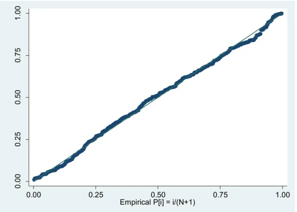
34 Figure A-‐1: F-‐distribution of transformed dependent variable

Figure A-‐2: Histogram of transformed dependent variable

0.

00

0.

25

0.

50

0.

75

1.

00

N

orma

l F

[(cycl

e

to

w

o

rksq

rt

-m)/

s]

0.00 0.25 0.50 0.75 1.00

Empirical P[i] = i/(N+1)

0

2

4

6

D

en

si

ty

.1 .2 .3 .4 .5

(35)

35 Figure A-‐3: Two-‐way scatter plot of cycle to work sqrt with creative industry sqrt

.1

.2

.3

.4

.5

C

ycl

e

to

w

o

rk

sq

rt

.1 .2 .3 .4 .5

(36)

36 Figure A-‐4: Map of square root of percent cycling (dependent variable) by MSOA3

(37)

(38)

38 Figure A-‐6: Map of sqrt pct cycling with tube stations* and cycle hire docks by MSOA

(39)

(40)

(41)

41 Figure A-‐9: Map of model predictions of dependent variable by MSOA4

TRANS_Final_Burton_Allen.pdf

Table of Contents