1203.pdf

TABLE OF CONTENTS

PAGE

1.0 INTRODUCTION

1.1 Use of Aquifer Tracer Tests 1

1.2 Purpose of Present Study 2

2.0 PRINCIPUES OF CONTAMINANT TRANSPORT

2.1 Introduction 3

22 Groundwater Row Equations 3

2.2.1 Steady-State Saturated Flow 4

2.2.2 Transient Saturated Flow 5

23 Contaminant Transport Processes 6

2.3.1 Physical Processes 6

2.3.1.1 Advection 6

2.3.1.2 Hydrodynamic Dispersion , 7

2.3.2 Chemical Processes 8

2.3.2.1 Diffusion 8

2.4 The Advective-Dispersive Equation ^ ^ 9

3.0 FIELD TRACER TESTS

3.1 Types of Tracers 11

3.1.1 Temperature Tracers 12

3.1.2 Dye Tracers 12

3.1.3 Ionic Tracers 13

3.1.4 Radionuclide Tracers 14

3.2 Types of Tracer Tests 15

3.2.1 Single-Well Tracer Tests 15

3.2.2 Two-Well Tracer Tests 17

4.0 FIELD DATA COLLECTION

41 Description of Field Site 19

4.2 Tracer Test Procedure 23

4.2.1 WeUs 23

4.2.2 Equipment Used 25

TABLE OF CONTENTS (Cont'd)

PAGE

5.0 METHODS OF DATA ANALYSES

5.1 Description of Tracer Test Simulation 36

52 Tracer Transport Modeling 37

6.0 CONCLUSIONS 49

•

Rgure 3.1

nOURES

Single Well Tracer Test

PAGE

16

Rgure 3.2

Two Well Tracer Test

18

Figure 4.1

Site Location Map

20

Figure 4.2

Topographic Location Map

21

Figure 4.3

Site Map

22

Figure 4.4

Tracer Test Well Details

24

Figure 4.5

Tracer Test Control Box

26

Figure 4.6

Tracer Test Equipment Layout

27

Figure 4.7

Tracer Test No. 1 Breakthrough Curve

29

Figure 4.8

Tracer Test No. 2 Breakthrough Curve

31

Figure 4.9

Observed Recovery Well Drawdown

34

Figure 5.1

Pumping Stress at Screened Interval

38

•

Figure 5.2

Two Well Tracer Test - 0 Hours

40

Figure 5.3

Two Well Tracer Test - 2 Hours

41

Figure 5.4

Two Well Tracer Test - 4 Hours

42

Figure 5.5

Two Well Tracer Test - 6 Hours

43

Figure 5.6

Two Well Tracer Test - 26 Hours

44

Figure 5.7

Percent Tracer Recovery vs. Time

46

Figure 5.8

Two Well Tracer Test - 240 Hours

47

APPENDICES

Appendix A Tracer Test No. 1 Data

Appendix B Tracer Test No. 2 Data

Appendix C Computer Modeling Data Files

1.0 INTRODUCnON

1.1 Use of Aquifi^ Tracer Tests

Due to the increasing number of lawsuits being ffled related to groundwater contamination sites,

predictions concerning the source of the contamination, its present course and future destination

have become the bread and butter of the subsurface hydrology business. In order to procure funding

for most contamination remediation efforts, culpable parties and those at risk by the migration of

the plume must be identified. The tools most often used to make these predictions are groundwater

models.

Mathematical groundwater models require that the user input many site specific aquifer parameters

that are used to describe the contaminant transport hydraulics and the subsurface conditions over

a site. These parameters include hydraulic conductivity, hydrodynamic dispersion, and contaminant

sorption and decay, either chemical or biological. ^

The hydraulic conductivity of an aquifer is a property of a water bearing formation that is defined

as the capacity of a porous medium to transmit water. The conductivity when used in model

calculations with the gradient and porosity determines the average direction and rate of groundwater

flow. The transport of solutes in the direction of the flowing groundwater is called advection.

Hydraulic conductivity can vary over a site not only in a horizontal plane but also vertically. In

order to obtain accurate modeling results over a large area with different conductivities, these

variations should be taken into account

^^^^^^W^^^—ffV***-a tr^^^^^^W^^^—ffV***-ansverse direction (perpendicul^^^^^^W^^^—ffV***-ar to the principle direction of flow). Hydrodyn^^^^^^W^^^—ffV***-amic dispersion

occurs due to mechanical mixing of the groundwater during advection and due to molecular diffusion

of the contaminant

Aquifer tracer tests may be performed to identify the spatial variability of hydraulic conductivity

within an aquifer, and to estimate the effective hydrodynamic dispersion using tracer breakthrough

data obtained during the test. This can be accomplished by packing off sections of fully penetrating

well screens and performing tracer tests at different vertical locations within the aquifer. By

separately analyzing these data sets, a set of hydraulic parameters can be estimated for each selected

screened interval.

12. Purpose of Present Study

The main objective of this study was to obtain a better understanding of the groundwater flow

pattern that is present at a particular area of a research site by measuring certain aquifer

parameters. The groundwater at the site had become contaminated with gasoline due to the failure

of underground storage tanks and associated piping. One of the first phases of the field study

involved the installation of groundwater monitoring wells; these included two pairs of wells

specifically designed for tracer studies. Two two-well field tracer studies were then performed using

each pair of welk.

The tracer tests had three objectives: (1) estimate aquifer parameters of the area in question, (2)

2.0 PRINCIPLES OF CONTAMINANT TRANSPORT

2.1 Intiodiictioii

In order to adequately understand contaminant transport in groundwater, the processes and

equations that are used to describe groundwater flow must be studied. The groundwater flow

equations form the basis for the transport equations because the bulk of the contamination in the

groundwater will propagate in the direction of and at a velocity equal to the average linear

groundwater velocity. This process is known as advection.

In addition to advection, localized processes that affect the transport of solutes within a groundwater

system are also very important to contaminant transport modeling. The phenomena of contaminant

dispersion, sorption, and reaction are included in the contaminant transport equations to further

describe these additional transport processes. The correct inclusion of these properties into a

model is essential to adequately describe the location, shape, and concentration of a propagating

contaminant plume.

22, Groundwater Flow Equations

The derivations of the equations used in groundwater flow applications are based on the

conservation principles dealing with mass, momentum, and energy. The basic law of flow is Darcy's

law. When Darcy's law is combined with an equation of continuity that describes the conservation

of fluid mass during flow through a porous medium, a partial differential equation of flow is the

result (Freeze and Cherry, 1979). Different forms of the flow equation result for steady-state,

The following sections review the three most commonly used forms of the groundwater flow

equations. The sections are a summary of Chapter 2, Section 2.11, "Groundwater" by R. Allan

Freeze and John A. Cherry (1979).

22.1 Steatty-State Saturated Flow

The equation of groundwater flow under steady-state conditions through an anisotropic saturated

porous medium:

i(K,!L)+i(is*) + i(K,^) = o (1)

dx. dK dy dy dz dz

The terms x and y refer to the principal horizontal axes with z representing the vertical axis. The

hydraulic head at any point in the three-dimensional flow field is represented by h. The subscripted

value of hydraulic conductivity, K, refers to the hydraulic conductivity in the direction of the three

principle axes.

\.

For the case of an isotropic medium, the hydraulic conductivities in the x, y, and z directions will

be equal, ie., K^^ = IC = K^.. Further simplification of the equation is possible if it can be assumed

that the aquifer medium is homogeneous as well.

Therefore, for the case of steady-state flow through a homogeneous, isotropic medium the equation

reduces to:

^h 4. ^h 4. ^ = 0 (2)

ax^ ay2 az2

This equation is known as the Laplace equation. The solution to the equation, the function h(x,y,z),

is the hydraulic head, (h), at the point (x,y,z) in the flow field. The usual application of this

equation is to a field site that has been divided into a 2-dimensional grid with each point in the grid

-\

of the hydraulic head, is then calculated for a range of depths (z) within the aquifer. Contour maps

of the local groundwater equipotential lines at specific depths (z) within the aquifer, can be then

generated.

?.?..?. Transient Saturated Row

For the case of a transient flow condition, the time rate of change of the hydraulic head will be

changing with time and must be accounted for in the equation. The groundwater flow equation used

to describe transient flow through a saturated anisotropic porous medium is as follows:

3 , 3hv 3/3h. d . 3h. 3h

_ (K, _) + _ (Ky _) 4. _ (K, !i) = S3 _ (3)

dx. ax dy dy d^ 3^ 3t

The term S^ is the specific storage term defined as the volume of water that a unit volume of a

saturated aquifer releases from storage under a unit decline in hydraulic head. The dimensions of

S^arepL]-!. \

For the special case of homogeneous and isotropic media, the equation reduces to:

3^h + 3^h ^ d^h — S3 3h ^4\

3x2 g^ gjj2 K a

Further reduction of the equation is possible for the special case of a horizontal confined aquifer

of thickness b. The storage coefficient, S, is defined as:

S = S3b (5)

In words, the storage coefficient or storativity of a saturated confined aquifer is the volume of water

that is released fi'om storage per unit surfece area of aquifer per unit decline in hydraulic head. The

The transmissivity, T, of a confined aquifer is a parameter used as a measure of the available yield

of a confined aquifer. T is defined as:

T = Kb (6)

The dimensions of transmissivity are [L'^/T].

Inserting the storage coefficient and the transmissivity into the equation, and assuming a

2-dimensional analysis is required, the equation for the special case of a horizontal confined aquifer

of thickness b, reduces to:

6^h ^ d^h _ S dh ^j\

ax^ dy^ T a

The solution to the equation, h(x, y, t) predicts the groundwater hydraulic head at any point on a

horizontal plane through the aquifer at any time, t.

23 Contaminant Transport Processes

23.1 Physical Processes

23.1.1 Advection

Advection is the process by which a dissolved solute or contaminant is carried by and in the direction

of the flowing groundwater. The bulk of the contamination is transported by this process.

The rate of the transport is equal to the average linear groundwater velocity, v, where v = v/n, v

23.12. HydnDdynamic Dispersion

Dispersion is a mixing process that causes the spreading of the contaminant from its advective path.

This phenomenon is caused in part by mechanical mixing and in part by molecular diffusion from

thermal-kinetic energy of the solute. The spreading causes dilution of the contaminant The

dispersion caused by mechanical mixing of the groundwater alone is called mechanical dispersion.

On a microscopic scale, mechanical dispersion is caused by three processes. The first is mixing of

the molecules due to the varying velocities of the molecules in the individual pore spaces between

particles. This is due to the frictional forces exerted on the molecules from the media. The second

process is caused by the varying pore sizes between media causing the molecules to move at different

pore velocities around the particles. The third process is related to the irregular and differing

shapes of the pore channels.

The spreading of the contaminant in the direction of the bulk of the flowing groundwater is called

longitudinal dispersion, whereas spreading in directions perpendicular to the direction of

groundwater flow is referred to as transverse dispersion. As can be expected, the dispersion in the

longitudinal direction is usually much larger than its transverse counterpart.

When using a 2-dimensional contaminant transport model, if the principal axes are aligned with the

direction of flow, the x direction, the dispersion in the x direction is the longitudinal dispersion and

For the one-dimensional case, the coefficient of hydrodynamic dispersion can be expressed in terms

of two components (Freeze and Cherry, 1979):

Dj = a«v + D* (10)

where: D^ is the coefficient of hydrodynamic dispersion, [L^/T]

a* is the dispersivity, [L]

D* is the coefficient of effective molecular diffusion for the solute in the porous medium,

[L2/T]

V is the pore velocity in the longitudinal direction, [L]

When doing transport modeling in 2 and 3-dimensions, the dispersion terms for each of the principle

directions are used along with all the off-diagonal terms, ie., D^ Dyy, D^, D^ Dy^ D^, D^ Dy^,

and D^y. Equations for all six dispersion terms can be found in Chapter 7-3 of Bear, 1979.

23.2 Qiemical Processes

232.1 Diffusion

Molecular diffusion is a microscopic physicochemical mixing process caused by varying concentration

gradients. Diffusion in solutions is the process whereby ionic or molecular constituents move under

the influence of their kinetic activity in the direction of their concentration gradient (Freeze and

Cherry, 1979). During fluid motion, such as flowing groundwater, diffusion acts as an additional

mechanism to provide solute mixing.

The coefficient of molecular diffusion, D, comes &om Pick's first law which can be stated as follows

(Freeze and Cherry, 1979):

F = -D(dC/dx) (11)

where: F = mass flux of the solute, [M/L^

D = aqueous diffusion coefficient, [L'^/T]

C = solute concentration, [M/L^]

dC/dx = concentration gradient, [M/L ]

The diffusion coefficients for ions in aqueous solutions have been well documented and are available

in many standard chemistry textbooks. Some of the major ions in groundwater (Na"*", K"*", Mg"*"^,

Ca'''^ Cr, HCO3", SO^'*''^) have diffiision coefficients in the range of 1 X 10'^ to 2 X 10"^ m/s @

25 degrees Celsius (Freeze and Cherry, 1979). The coefficients are temperature dependent For ions

in porous media, however, the "apparent" diffusion coeffiicients are much smaUer than in water due

to adsorption and because the ions follow longer paths of diffusion caused by the presence of

particles in the solid matrix (Freeze and Cherry, 1979).

The apparent diffusion coefficient for nonadsorbed particles in porous media, D , is represented by

the following (Freeze and Cherry, 1979):

D* = S>D (12)

where 2> is an empirical coefficient which accounts for the effects of the solid matrix on the

diffusion. In laboratory studies, experimental values for 2) of between 0.5 and 0.01 have been

commonly observed (Freeze and Cherry, 1979).

2.4 The Advective-Dispersive Equation

is called the advective-dispersive equation. One commonly used form of this equation is given below

(for a complete derivation of the advective-dispersive equation, see Freeze and Cherry, 1979,

Appendix X):

ac r a'^c a^c a^c-i r ac ac ac -i

_=LDx _ + Dy _+ D, _j-[v^_ + Vy_ + v,_J -q/n (13)

at ds? dy^ d^ ax ay az

where: C = concentration of solute = mass of solute/unit volume of solution

q = rate of change of solute mass (sink)/unit volume of porous media

V = pore or seepage velocity

n = porosity of the media

D = (D^ D^ D2):dispersion coefficients

The sink term q refers to the rate of loss of mass of solute/unit volume of porous media. The

changes usually occurring to a dissolved contaminant in groundwater include sorption ontoylnto the

media and losses due to chemical reactions and/or biological degradation. The form of Equation

13 above assumes that the aquifer medium in question is homogeneous, isotropic, and saturated. The

flow conditions are assumed to be steady, and Darcy's Law is applicable. The equation also assumes

that the effective transport mechanisms present are advection and dispersion. The solution to

Equation 13 is a prediction of the concentration of the solute in question at a desired point in time

at a known location.

Solving the equation requires approximation of the partial differentials by iterative numerical

techniques using finite difference and finite element modeling or the use of analytical methods.

Some analytical solutions exist for cases such as tracer slug injection into a column, with and without

adsorption. (For a discussion of some of the currently available analytical solutions, see Section 7-9

in Bear, 1979.)

Equation 13 can be used to model a field tracer test by predicting the expected concentration of the

tracer as a function of time at the point of withdrawal assuming that the tracer is conservative. By

attempting to match the model results with the actual field breakthrough data, the aquifer

parameters that were estimated in order to run the model can now be determined more accurately.

Numerous model runs using different aquifer parameters may have to be made in order to achieve

a close match of the two data sets.

3Ja FIELD TRACER TESTS

3wl Types of Tracers

In their paper presented at a 1955 American Water Works Association meeting in Sacramento,

California, Warren J. Kaufman and Gerald T. Orlob discuss characteristics of an ideal groundwater

tracer. The authors site the following properties:

"

ͣ

ͣ

, \ " ;

_ͣ

\

ͣ

1. A satisfactory tracer should be susceptible to quantitative determination in very low

concentrations;

2. It should be entirely absent from the injected water or present only at low

concentrations in the displaced water;

3. It must not react with the injected or displaced waters to form a precipitate;

4. It must not be absorbed by the porous medium; and

5. It must be cheap and readily available.

Although the authors were referring to the tracing of groundwater movement under natural gradient

conditions for the purpose of watershed development and protection, their ideal tracer properties

Bear (1979) describes an ideal tracer as one that is inert with respect to its liquid and solid

surroundings and that does not affect the liquid's properties. In reality, however, the introduction

of a tracer into an aquifer does cause changes to the groundwaters' density and viscosity. In

situations where an artificial tracer is introduced in relatively low concentrations, the ideal tracer

assumption may be appropriate. In other cases for example where the groundwater density may vary

significantly within the aquifer due to seawater intrusion, the assumption that the chloride

introduced by the intrusion will behave as an ideal tracer is not valid.

3.1.1 Temperatoie Tracers

Water temperature has the potential to be a fairly useful tracer although it has not been used

extensively. The method seems to have the most potential in granular media, firactured rock, and

karst regions (Davis et al., 1985). Temperature tracers have been used to trace vertical groundwater

movement in boreholes (Keys and MacCarey, 1971; Sorey, 1971), and to trace the artificial recharge

of a naturally heated lake water into an aquifer forriiation (Keys and Brown, 1978).

A problem with using temperature tracers exists, however, due to changes in the density and viscosity

of groundwater caused by temperature changes. These changes affect the flow rate and the direction

of the groundwater. Experiments conducted in a laboratory setting have attempted to illustrate

these effects (Davis et al., 1985). In order to minimize these negative effects, the temperature

difference between the tracer and the background should be kept as small as possible.

3.L2 Dye Tracers

Various organic dyes have been used for surface water and groundwater tracing since the late 1800's

with extensive use of fluorescent dyes beginning around 1960 (Davis et al., 1985). Dyes are easy to

use and have high detectibility, however, dyes travel slower than water due to adsorption and

therefore are not conservative as are ionic or radioactive tracers (Davis et al., 1985). Some of the

more commonly used dyes include fluorescein, pyranine, lissamine FF, rhodamine WT, and sulfo

rhodamine B. A number of factors have been shown to interfere with the measurement of

fluorescent dye concentration. These factors include temperature, pH, alkalinity, and salinity (Davis

et al., 1985). Sorption and toxicity problems with the dye tracers have also been researched (Smart

and Laidlaw, 1977).

Although dyes are more often used for surface water work, groundwater tracer experiments using

dyes have been conducted. An experiment conducted using three different fluorescent dye tracers

ran into problems when the injection slug of tracer was introduced too slowly and the dye was

diluted below detection limits (Naymik and Sievers, 1985). Better results from groundwater tracing

experiments can be obtained using conservative ionic or radioactive tracers.

3.13 Ionic tracers

\

Ionic compounds have been employed extensively and Successfully as groundwater tracers. The most

common and successful species used include chloride (CI"), bromide (Br"), lithium (Li"*"), ammonium

(NH^"*"), magnesium (Mg'*"''), potassium (K"*"), iodide (I"), sulfate (S04~), organic anions (such as

benzoate), and fluorinated organic anions (Davis et al., 1985). Ionic tracers, especially anions, are

considered to be conservative under most aquifer conditions. Anionic tracers are considered to be

conservative because the anions usually will not decompose in the system, adsorb to the media, nor

undergo emion exchange.

Cations, on the other hand, have the tendency to react with the media by undergoing the process

of cation exchange. This process occurs when naturally occurring background cations such as

sodium and calcium are displaced and forced into solution by the introduction and the binding of

Under certain conditions, more than one ionic tracer should be used. In one of his papers on the

3-dimensional natural gradient tracer tests that were performed at the Canadian Forces Base Borden

in Ontario, Canada, Freyberg (1986) discusses his reasons for using both chloride and bromide as

tracers. The author explains that a contaminant plume containing elevated levels of chloride ions,

but negligible levels of bromide ions, is emanating from an abandoned landfill upgradient from the

experimental site. The plume is thought to lie below the experimental zone. By inspecting the

chloride:bromide concentration ratios for the samples collected during the experiment, the author

was able to identify the intersecting regions between the experimental and the landfill plumes.

Freyberg (1986) also discusses how the use of the two nonreactive tracers thought to behave so

identically, provided additional information on aspects of sampUng variability. Different analysts

performed the data reduction for the two ions which allowed for observation of any variability by

the analyst's judgment

In their paper on groundwater contaminant migration from a landfill, Sudicky et al., (1986) describe

their reasons for choosing a chloride tracer for their field experiments with a natural gradient

dispersion test The authors cite that chloride was selected for the tracer because it meets most of

the criteria for an ideal tracer. In addition, chemical analyses for chloride ion are inexpensive with

analytical precision being generally high.

3.1.4 Radionuclide Tracers

The majority of radioactive tracers used today are from sources of contamination already present

in the aquifers. According to one source the use of artificially introduced radioactive tracers has

declined in many countries including the United States (Davis et al., 1985). Field detection of

radioactive tracers is possible at very low concentrations using fairly simple field equipment (Molz

et al., 1986). In addition, tracers can be selected that have half-lives so short that they are

essentially decayed after a few hours or a few days (Davis et al., 1985).

32 Types of Tracer Tests

It is generally agreed that tracer tests are currently the most reliable field methods for obtaining

data to describe dispersion in groundwater (Molz et aL, 1986). All tracer tests fall into one of two

categories; forced or natural gradient

Natural gradient tests involve the introduction of a conservative tracer into an aquifer and

monitoring the movement of the tracer under natural groundwater flow conditions. Because the

natural movement of groundwater is in most cases very slow, the projected duration of a natural

gradient tracer test over even a small horizontal distance can take from weeks to months to

complete. For this reason, forced gradient tests have been developed to allow tracer tests to be

completed within much shorter time frames.

Forced gradient tracer tests introduce much higher hydraulic gradients than are present under

natural flow conditions into the aquifer through the use of one or a series of pumping wells. The

increased groundwater flow rate which is a response to the pumping stress, forces the groundwater

to flow much faster than it would under natural flow conditions allowing a shorter duration test.

The two most common types of forced gradient tracer tests are single-well and two-well tests.

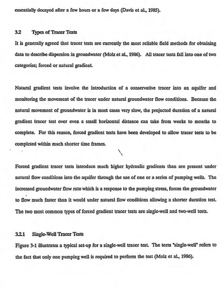
32.1 Single-Well Tracer Tests

Figure 3-1 illustrates a typical set-up for a single-well tracer test. The term "single-well" refers to

WITHDRAWAL

CoutW

Qout

Ti n 1 n n ) i i'l r

SAMPLING PORT

INJECTION

Cin(t)

Qin

/^77^7^T^777

\

WATER TABLE

ͣ

ZONE OF INJECTED TRACER

FIGURE 3.1

SINGLE WELL TRACER TEST

(Ref: Davis etaU 1985)

During the test, a tracer solution having a known concentration, Cjn(t), is injected at a known rate,

Qjjj, for a known period of time into a well that is fully penetrating and screened over the entire

thickness of the aquifer. After a certain period of time, the flow may be reversed and the tracer

solution is pumped from the welL The recovered tracer solution pumped from the well at

concentration, Com(t), may be used to develop a breakthrough curve of concentration vs. time data.

In many cases it may be useful to calculate the percentage of tracer recovered.

In cases were the vertical conductivity distribution in the aquifer is desired, multi-level sampling

wells can be used in conjunction with the injection well. Concentration vs. time measurements are

then made at the different isolated points in each observation well during the experiment (Molz et

al., 1986). Horizontal hydraulic conductivities are estimated using the tracer travel time and tracer

concentration data measured at each vertical sampling interval

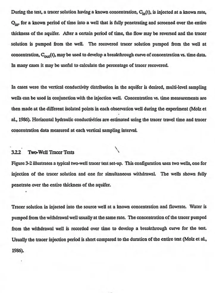
3.2.2 Two-Well Tracer Tests "^

Figure 3-2 illustrates a typical two-well tracer test set-up. This configuration uses two wells, one for

injection of the tracer solution and one for simultaneous withdrawal. The wells shown fuUy

penetrate over the entire thickness of the aquifer.

Tracer solution in injected into the source well at a known concentration and flowrate. Water is

pumped from the withdrawal well usually at the same rate. The concentration of the tracer pumped

from the withdrawal well is recorded over time to develop a breakthrough curve for the test.

Usually the tracer injection period is short compared to the duration of the entire test (Molz et al.,

WITHDRAWAL

Cout(t)

Qout

PUMPED WELL

11 rn n

INJECTION

Cin(t)

Qin

kt

-© (E^-S

n n iT/j 1 / n i i in

y.

_ ^

INJECTION WELL

T-i 11 n I) I n 11 7 r

N

\

.^rsfl

_{M_8L£}

FIGURE 3.2

TWO WELL TRACER TEST

(Ref: Davis et aU 1985)

Two-well tests may be carried out in either a recirculating or non-recirculating mode (Molz et al.,

1986). In the recirculating mode, the water pumped from the withdrawal well is reinjected back into

the injection welL The injection concentration of tracer solution in this case will be equal to the

sum of the tracer solution plus the concentration of the withdrawn water from the aquifer.

By using multi-level observation weUs to collect groundwater samples during the test, horizontal

conductivities may be estimated from the concentration and time data.

4J0 FIELD DATA COLLECnON

4^1 Description of Field Site

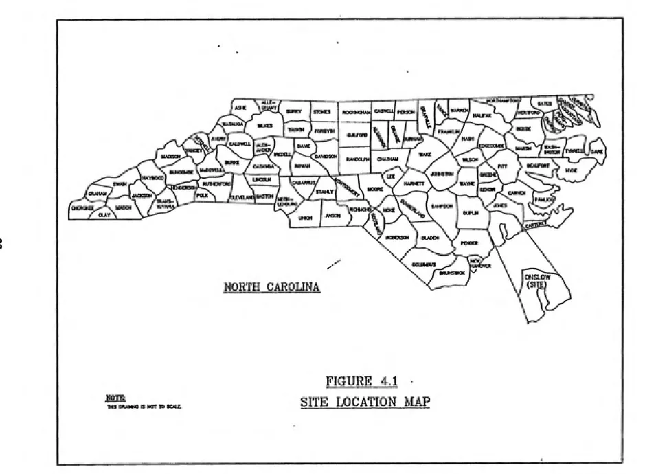
This study was conducted at the Terrawa Terrace site located at Camp Lejeune, North Carolina

(Figures 4.1, 4.2, and 4.3). Geologically, the site is located within the North Carolina coastal plain

which is characterized by sandy soils and a shallow groundwater table. Boring logs and published

soil data maps indicate that approximately 200 feet of fine to medium grained sands mixed with

varying amounts of clay (Mayer and Miller, 1988) comprise the surficial unconfined aquifer which

is underlain by a confining layer. The average depth to groundwater at the site is approximately 25

feet

A gas station at the site has been identified as the source of subsurface gasoline contamination

caused by leaking underground storage tanks and associated piping. It is estimated that

approximately 7400 gallons of leaded and unleaded gasoline were released between September 1985

g

CASWui

ROCKtNGHAM PEHOTH ItERIFORD

\\h-WATAUOA

YAOKIM 1 fORSYTO

AStRY

<=*">»*"• *l£3<- DAME

njOECOMBEl „^^„ ^WAW-

DAVIDSON WL5QN

CATATOA UcOOWELl

JOHNSTON I I OR

UNCOIN

CABAnnus RUTWRFOBD

POLK

5TANLY OARVEH

CRAHAM PAMUCO

TRAHS-YIV,

CHEROKEE^^'^ UACON

CLAY

mCHMONO^^ HOKE

^WSON

RENDER

lAHOVER

ONSLOW

(SITE

NORTH CAROLINA

mm.

im iNAwm n NOT TO acAii.

FIGURE 4.1

Ai

^'

^

Pointy

MORGAN

^

SCALE 1:50,000

0

n: :e

2 MILES

3

CAUP LEUSUNE SPECIAL UAP

NORTH CAROLINA - EAST COAST

1976

PREPARED BY DMATC AND DMAHC

PUBUSHED BY THE

DEFEMSE MAPPING AGENCY HYDROGRAPHIC CENTtR

WASHINGTON, D.C.

FIGURE 4.2

A-2-J I

A-1

ASPHALT-^^

STATION UNION 76

ASPHALT

OB-11

PUMP

ISLAND

UNDERGROUND

TANKS

OB-8

USMC STORM

LEGEND:

-- EXISTING WELLS

A BENCHMARK

NOTE: TRACER TEST NO. 1: INJECTION WEa A-13

WITHDRAWL WELL A-11

TRACER TEST NO. 2: INJECTION WELL A-12

WITHDRAWL WELL A-10

FIGURE 4.3

SITE MAP

After the release was discovered, a consultant was retained to perform groundwater contamination

assessment and remediation services. Eleven monitoring wells were installed during the initial

phase of the investigatioiL Eventually, a pump and treat system designed to remove free gasoline

from the surface of the water table and to remove dissolved gasoline constituents from the

groundwater was designed and constructed at the site. The underground storage tanks were

removed in May 1987 and the area served as a groundwater contamination research site.

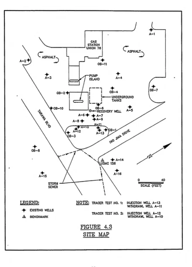
During July and August of 1987, a UNC research team installed 16 additional groundwater

monitoring weUs including twelve multi-level sampling wells. A map of the site included as Figure

4.3 shows the well locations as of December 1987.

42, Tracer Test Procedure

4.2.1 WeUs

Two two-well tracer tests were performed at the site using two different pairs of weUs. Test No.

1 was conducted on August 25, 1987 using wells A-11 and A-13. Test No. 2 test took place on

November 12,1987 using wells A-10 and A-12. During the two tracer tests, the existing groundwater

recovery and treatment system continued to operate. The average groundwater pumping rate from

the recovery well as measured before the start of each tracer test was approximately 10 gpm. It is

assumed that this average rate was maintained during the two tests.

Each pair of welk consists of an injection well and a withdrawal well. The injection wells, weUs

A-12 and A-13, are constructed of 48 feet of 2 inch diameter stainless steel casing with 2 feet of slotted

stainless steel screen. The withdrawal wells, wells A-10 and A-U, are constructed of 50 feet of 4

inch diameter stainless steel casing with 2 ft. screen sections. Construction details of the two

INJECnON WELLS

STEEL RISER: 6" DIA. WITH LOCKING CAP

WITHDRAWAL WELLS

STEEL RISER: 4" DIA. WITH LOCKING CAP

'^^S^

*.**¥.>)

5S5SSSSS5?3SSSSS55SSSSS5S5S5S5S5S5SSSS5SSS5SS^S5S5?^!SS

CONCRETE COLLAR EXTENDING'

2' BELOW GROUND SURFACE.

COLLAR IS TAPERED, 18" DIA.

AT SURFACE. AND SLOPED TO

_GRADE AWAY FROM CASING.

GROUT BACKRLb NEAT CE.MENT

SEAL OF 1/2' BENTONITE PELLETS

SAND

BACKFILL-CASING: 4" DIA., TYPE 304

STAINLESS STEEL, FLUSH

THREADED, SCH 10

CASING: 2" DIA., TYPE 304

STAINLESS STEEL. FLUSH THREADED,

SCH 10

SCREENED SECTION: 2' LENGTH, 4"

DIA., TYPE 304 STAINLESS STEEL

SCREEN, WIRE WOUND. FUT BOTTOM

ON SCREEN SECTION.

SCREENED SECTION: 2" LENGTH, 2'

DIA.. TYPE 304 STAINLESS STEEL

SCREEN, WIRE WOUND. FLAT BOTTOM

ON SCREEN SECTION

L

55ES555555S5^

LT.*^

>.•>

5^r^

liQIE: CRAVING IS NOT TO SCALE

FIGURE 4.4

TRACER TEST WELL DETAILS

4:12 Equipment Used

In order to be certain that the pumps controlling the rate of tracer solution injection and the rate

of groundwater withdrawal are producing identical yields, it is imperative during a tracer test that

the injection and withdrawal flow rates be continuously monitored. In addition, sampling ports must

be conveniently located to allow for frequent sample collection of tracer solution and withdrawn

groundwater. With these ideas in mind, a tracer test control box was designed and constructed as

shown in Figure 4.5.

To monitor and control the groundwater withdrawal rate from the pumping well, the box contained

a flowmeter, a sampling port, and control valve. The groundwater was pumped from the withdrawal

well using a stainless steel submersible pump. The tracer solution was pumped from the mixing

tanks to the injection well via the magnetic motor pump housed in the control box. The injection

line was also equipped with a flow control valve, a sampling port and an instantaneous readout

flowmeter. An inline filter housing was plumbed in for use during a subsequent experiment. A filter

cartridge was not placed in the housing during the two tracer tests. An equipment layout illustrating

the hardware setup during the two tests is shown in Figure 4.6. The hardware setup for the two

tests was identical.

4.23 Tracer Test No. 1

Tracer Test No.l was started at approximately 11:00 am on August 25, 1987 and continued for a

duration of 25.5 hours. Prior to the start of the test, 90 gallons of tracer solution were prepared

using groundwater from the site. A measured amount of sodium chloride was added to bring the

concentration of the solution equal to 250 mg/L of chloride plus whatever background chloride

concentration was present (approximately 15 mg/L Q-). A total of 85.16 grams of chloride were

TO OUTFALL

TO

INJECTION

ͣ

UNE

-TV

-GILMONT FLOW METER

DWYER FLOW METER--PVC PIPE

X

INJECTION FLOWRATE CONTROL VALVE

5

COLE-PARMER

MAGNETIC MOTOR PUMP

PUMP

2

T

PORT \

O

FLOWRATE CONTROL

• STAINLESS

STEEL PIPE

FROM WITHDRAWAL

ͣ

0.2 ii RLTER HOUSING

(TEFLON)

50

SCALE (FEET)

FIGURE 4.5

TRACER TEST CONTROL BOX

TRACER SOLUTION

VESSELS

TRACER SOLUTION

PUMPED

GROUND-WATER TO OUTFALL

CONTROL

BOX

PUMPED —

GROUND

WATER

— 1/2"

STAINLESS

STEEL

UNES

TRACER SOLUTION

ͣ

2" INJECTION

ͣ

4' WITHDRAWAL ^"^^

WEIL

NOTE: PLAN MEW NOT TO SCALE

FIGURE 4.6

Tf^s-The tracer solution was injected via the injection well, well A-13, at a flowrate of 0.25 gallons per

minute (gpm) and the groundwater was withdrawn from the pumping well, well A-11, at a flowrate

of 0.25 gpm. The flow rate was controlled by fine tuning with the control valves. When all of the

tracer solution was injected, the influent line was switched to vessels containing background

groundwater. For the duration of the test, the background groundwater was continuously injected

at the 0.25 gpm flowrate to maintain a steady state system.

Groundwater samples from the pumping well were collected every 15 minutes for the duration of

the test. A mobile on-site laboratory was set up to analyze the samples for chloride concentration.

A complete listing of the data collected from Tracer Test No. 1 is included as Appendix A. The

analytical method used to analyze the samples for chloride concentration was Method A

(Mercurimetric Titration), ASTM D 512 - 80.

By reducing the collected data, the breakthrough cti^^e, shown in Figure 4.7, was developed.

4i4 Tracer Test No. 2

Tracer Test No. 2 was started at approximately 6:34 am on November 12, 1987 and continued for

a duration of 30 hours. Prior to the start of the test, 120 gallons of tracer solution were prepared

using groundwater from the site. A measured amount of sodium chloride was added to bring the

concenfration of the solution equal to 250 mg/L of chloride plus whatever background chloride

concentration was present (15 mg/L C1-). A total of 113.55 grams of chloride were injected over the

duration of the test

The tracer solution was injected into the injection well, well 12, and the groundwater was withdrawn

from the pumping well, well 10, at a flowrate of 0.5 gallons per minute (gpm). The flow rate was

controlled by fine tuning with the confrol valves. As was done during the first tracer test, when all

E

z

g

H Z

u

o z o o

u

Q q: o

-J

I

o

80

70

60

-50

40

30

20

10

-0 -ly

RESULTS FROM FIRST TRACER TEST

TRACER CONCEN. = 250 mg/L CHLORIDE

J

20

TIME IN HOURS

r

of the tracer solution was injected, background groundwater was injected at the same flowrate to

maintain a steady state system.

Groundwater samples from the pumping well were collected every 30 minutes for the duration of

the test. The mobile on-site laboratory used for Tracer Test No. 1 was used to analyze the samples

for chloride concentration. A summary of the parameters for Tracer Tests No. 1 and 2 is as follows:

Flowrate

Injection Well

Withdrawal well

Radial Distance

Test Duration

Tracer Injection Time

Injected tracer volume

Tracer concentration

Mass of Injected Tracer

TRACER TEST NO. 1

0.25 gpm

A-13 (2" O.D.)

A-11 (4" O.D.)

3.84 feet

25.5 hours

6 hours ^\

90 gallons

250 mg/L chloride

85.162 grams

TRACER TEST NO. 2

0.5 gpm

A-12 (2" O.D.)

A-10(4"O.D.)

2.63 feet

30 hours

4 hours

120 gallons

250 mg/L chloride

113.549 grams

By reducing the collected data, the breakthrough curve, shown in Figure 4.8, was developed. A

complete listing of the data collected from Tracer Test 2 is included as Appendix B. The analytical

method used to analyze the samples for chloride concentration was Method A (Mercurimetric

Titration), ASTM D 512 - 80.

1^

-I

\

E

z

g

z

u

o z o o

u

Q

o: o

_J

I

o

80

70

-60

50

-40

30

RESULTS FROM SECOND TRACER TEST

TRACER CONCEN. = 250 mg/L CHLORIDE

20

10

-20

TIME IN HOURS

43 Discussion of Results

The test parameters selected prior to Tracer Test No. 1 were chosen using the most reliable site

data available. The breakthrough curve obtained from the test data was not as complete as it could

have been because the "tail" of the curve did not approach the abscissa asymptotically. Additional

data should have been collected until the flattening of the curve had been obtained. Although the

samples collected were being analyzed in the field within a short time, the duration of the test, the

fi-equency of sampling, and the field laboratory conditions which prohibited sample analysis at night,

all contributed to misjudging what the true length of the test should have been.

In order to correct this problem for Tracer Test No. 2, the injection and withdrawal flow rate was

doubled to allow for the capture of more tracer solution in a shorter period of time. It was ako

decided to lengthen the minimum duration of the test to 30 hours. By incorporating these two

changes into the tracer test procedure, the plotted breakthrough data from Test No. 2 as shown in

Figure 4.8 appear to be more representative of a complete test

It is interesting to note the percent of the total mass of injected chloride recovered from each test;

37 percent for Tracer Test #1 and 52 percent for Tracer Test #2. With both injection and

withdrawal wells only about three feet (one meter) apart, the tracer solution injected in the center

of the screened interval of both of the injection weUs, the submersible pumps installed in the center

of the screened intervals of the withdrawal wells, and both wells having approximately the same

screened interval, it would seem logical to expect to recover most if not all of the injected tracer

during each of the tests.

Factors that could account for the difference in the amount of the tracer recovered between Test

#1 and Test #2 include the difference in the flow rates and the duration of pumping.

Another factor that may have influenced the tracer test results is the construction of the withdrawal

well for Test #2, well #A-11. The construction of this well is somewhat suspect due to problems

that occurred in the field during drilling. The completed depth of the well is approximately 18

inches less than the other weUs making the screened interval o&et somewhat as compared to the

other tracer wells. The percent of total mass of tracer recovered during Test #2 may have been

even greater if the injection well had been completed to the same depth as the withdrawal well.

Because the point of injection of the tracer was at 50 feet below grade under a standing water

column of approximately 25 feet, the tracer was injected under pressure. The hydraulics of injecting

0.25 to 0.5 gallons per minute of solution probably caused a radial flow of the solution to spread in

all directions. Whether the pumping stress caused by the withdrawal well was strong enough to

overcome the spreading of the tracer and pull it back toward the withdrawal well in the duration

of the test could account for the majority of the tracer loss.

\

The other obvious possible cause of tracer loss is the apparent pumping stress induced by the

recovery well located approximately 40 feet from the tracer wells. Water levels in the monitoring

wells as measured around the time of the first tracer test are shown on Figure 4.9. Using this data

and assuming that they are representative of steady state conditions and that the surface horizontal

gradient is approximately equal to the gradient at 50 feet below grade, an estimate of the horizontal

groundwater velocity in the vicinity of the tracer test wells can be calculated. Assuming a hydraulic

conductivity of 1 x 10 ft/sec (Mayer and Miller, 1988), an effective porosity of 0.40 (typical for

sandy coastal plain aquifers), a horizontal gradient in the vicinity of the tracer wells of approximately

0.018 (as estimated from Figure 4.9) and assuming Darcy's Law applies, the horizontal velocity can

then be calculated to be approximately 4.5 x 10"^ ft/sec. Assuming that the duration of the tracer

4^

16-1

0 16

SCALE (METERS)

1—I—I—r

J___I___I___I___I___L

FIGURE 4.9

OBSERVED RECOVERY WELL DRAWDOWN (IN METERS)

withdrawal well is located between the recovery well and its respective tracer injection welL If the

groundwater moved 6 inches in the direction toward the pumping well during each tracer test, one

would ©q)ect that this would assist in the capture of the tracer as opposed to causing the tracer to

be lost

The loss of the tracer could also be attributed to the presence of a vertical gradient in the vicinity

of the tracer test wells caused by the recovery well. In their modeling study of the hydraulics of the

pumping recovery well at the Camp Lejeune site, Mayer and Miller (1988) determined that a vertical

gradient did exist in the vicinity of the pumping well. The recovery well is screened at an interval

of approximately 40 to 45 feet below grade (Mayer and Miller, 1988), whereas the tracer test wells

are screened at 50 feet below grade and are located approximately 40 feet away from the recovery

well. Using the data from the simulated hydraulic heads as a function of elevation in the immediate

vicinity of the recovery well (Mayer and Miller, 1988) at a depth of 50 feet below grade, a vertical

gradient due to the recovery well pumping stress of approximately 0.0075 and a vertical velocity of

1.8 X 10 ft/sec can be estimated. The actual vertical gradient in the vicinity of the tracer wells will

be significantly less than at the recovery well as demonstrated in the areal graphical vertical head

distributions shown in the referenced paper. Therefore, during the 30 hour duration of the tracer

tests, it is estimated that the groundwater may have moved less than 3 inches vertically upward due

to the stress induced by the recovery well. The stresses induced by the recovery well probably did

have some effect on the movement of the tracer and could be accountable for some of the losses.

However, these losses as estimated herein appear to be negligible. The effects of density and

temperature differences were assumed to be negligible and were not taken into account in the

5.0 METHOD OF DATA ANALYSIS

5.1 Descriptioii of Ttaca Test Simulatioii

By using equations that attempt to simulate the breakthrough response, certain aquifer parameters

can be estimated. These equations are usuaUy solved using computer models. To estimate the

aquifer parameters using the tracer test breakthrough data, the preferred method of analysis was the

use of a readUy available public domain computer based curve matching model. With the assistance

of the International Groundwater Modeling Center (IGWMC) of the Holcomb Research Institute

at Butler University in Indianapolis, Indiana, the available models were identified. The list was

narrowed to one potential model, since analytical solutions have not been derived for conditions

similar to those investigated in this study. The model chosen for further evaluation was the

Computer Aided Tracer Test Interpretation Code, "CATTI" by J.P. Sauty and W. Kinzelbach, May

1988. The model is a computer code used to estimate aquifer transport parameters from tracer test

data by either manual adjustment or by automatic least-square determination. CATTI is a

nonproprietary code and is distributed through the IGWMC

Since the CATTI documentation did not provide a complete description of the underlying theory

of the model, the author of the model, J. Sauty, was contacted in France. He was able to supply an

additional reference (Sauty and Kinzel, 1988) which was carefully reviewed. Upon further review,

it was determined that the CATTI program was an empirical solution, which was based upon a

radially symmetric flow field. This was a clear violation of the conditions under which the

experimental data was collected.

Also, CATTI simulates breakthrough data from either instantaneous or continuous tracer injection

tests for the case of radial flow, however, the actual field tests involved injecting tracer over a 4 to

6 hour period. The injections were neither instaneous nor continuous. After reviewing these model

limitations an alternate scheme was sought.

52, Tracer Transport Modeling

Since efforts to locate a satisfactory analytical solution failed, a numerical approach was deemed

necessary. Several models exist in the public domain to simulate the tracer tests performed.

The groundwater hydraulics in the vicinity of the tracer wells were simulated using the

McDonald-Harbaugh "Modular Three-Dimensional Finite-Difference Ground-water Flow Model" (McDonald

and Harbaugh, 1988). In order to run this model, a finite difference grid was set up around the

vicinity of the pair of wells used for Tracer Test #1. The model grid was set up with 17 columns

with a total dimension of 33.83 feet, 34 rows with a total dimension of 38.83 feet, and nine layers

with a total dimension of 134 feet The grid was set up with varying size cells with the sizes of the

cells decreasing as they approach the location of the wells. Cell sizes ranged firom 2x2 inches to

6x6 feet The ocact dimensions of the model grid including each cell block are included in the

MAIN.DAT input file included in Appendix C. Using the site parameters for hydraulic conductivity,

the model was run to simulate steady state flow conditions. The model was set up with a constant

head boundry on the perimeter and no flow boundaries on the top and bottom. The screened

interval was used as a separate layer. The simulation was run neglecting any effects from the

recovery welL

The hydraulic gradient as calculated from this three dimensional groundwater flow simulation for

the screened interval of both wells is shown in Figure 5.1. According to the modeling results, no

U I I II I II III I m I I 11 H I 11 I III 111 H I II III 11 HI I II I 11 111 I H II H 11 11 H 11II11

o o

6 66

J^

o o

-111 nil...mil iiiniimiimii iiiliiiimiiiiiiiiiiiiiiiiiiiiiiiiiiii

in

ID

LU

Assuming that the tracer particles move perpendicularly toward the equipotential lines, it appears

from the results shown in Figure 5.1, that the tracer would indeed move radially outward from the

well.

To track the path of the particles and to generate time of travel information to confirm whether the

percentage of tracer recovered during the tracer tests was reasonable, the three dimensional particle

tracking program, MODPATH, was used. MODPATH (Pollock, 1989) is a post-processing package

developed to compute three dimensional path lines based on steady-state simulations obtained from

the U.S. Geological Survey Modular Three-Dimensional Finite-Difference Ground-water Flow

Model.

MODPATH uses a semi-analytical partical tracking scheme based on the assumption that each

directional velocity component varies linearly within a grid cell. Given the initial position of a

partical anywhere in a cell, the coordinates of any other points along its pathinline within the cell,

and the time of travel between them, can be computed by the model (Pollock, 1989).

Data is input to MODPATH through a combination of files and interactive dialogue. The model

input data includes the input files BAS.DAT, BCF.DAT, WEL.DAT, OCDAT, SIP.DAT and the

output files BUDGET.OUT and HEAD.OUT used and generated in the execution of the Modular

Three-Dimensional Finite-Difference Ground-water Flow Model. MODPATH also requires the

data file MAIN.DAT. A detailed descriptiuon of the input parameters for these two files are

included in the model user manual (Pollock, 1989). A copy of each of the input files used to run

the simulation is included in Appendix C A companion program, MODPATH-PLOT, was used to

generate the graphical presentation of the MODPATH particle tracking output as shown in Figures

.fpwfflSWSRJ

t---_---1

L 3

ͣͣ

,____________________^---1

11 i- 1

All---1_________________________1

lLi-l.--l__

1

[

FIGUFE52

TWO WELL TRACER TEST - 0 HOURS

40

0 1 2 FEET

I.I I I iJ---1

s

_%

I I I I

2 FEET

nGURE5.3

TWO WELL TRACER TEST - 2 HOURS

0 1 2 FEET

1 I I I I I________I

FK3URE5.4