By: Sarah Flinn
Honors Thesis Economics Department
The University of North Carolina at Chapel Hill
April 2015
Approved:
Acknowledgements
I would like to take a moment to thank my faculty advisor, Brian McManus. He has provided
me with invaluable insight and support in my studies, and he has always pushed me to work and think harder. I would also like to thank Klara Peter, the Honors Thesis Director for the
Economics Department, for steering me in the right direction with my research. Finally I would
Abstract
This paper uses patient-level pooled cross sectional data from the National Ambulatory Medical
Care Survey (NAMCS) to study the impact on the adoption IT systems in the health industry (namely stand alone offices) in the form of Electronic Medical Record (EMR) systems. It also examines what physician characteristics make adoption more probable. When looking at patient
visits from the years 2005-2010, an OLS model shows that full EMR systems increase patient visit time by about 3%, however there is reason to believe that these results are biased due to
endogeneity in the EMR variable. Because EMR systems are not randomly assigned to physician offices, there is likely a link between the type of patients a physician serves, and that physician’s choice to adopt EMR systems. After using instrumental variables and a two stage least squares
regression, I am able to show that the adoption of EMR systems decreases patient visit time by 24.2%. The IV and 2SLS show that endogeneity exists within the EMR variable, and in fact
I. Introduction
It is obvious that technology is playing a large role in nearly all aspects of life in the United States. Up until recently however, the medical field has been slow to adopt IT systems in comparison to other industries due in part to high initial costs and slow financial returns
(Christensen 2007). While the economic benefits of adopting health IT may not be large, the social benefits that patients receive from Electronic Medical Records (EMRs) is thought to be
significant, and thus the driving force behind EMR adoption. Throughout my research, I examine the effect of EMR adoption on the time a patient spent with a physician per visit in an office setting. While it is intuitive that EMR systems would increase physician efficiency
through a reduction in paper work (for notes, labs, prescription orders, imaging etc.), a simple OLS model of patient visit time on EMR systems shows the opposite. While analyzing data from
visits in 2005-2009 with an OLS regression, full EMR systems increased the time of a visit by 3%. Although the results are statistically significant, they cannot be trusted completely due to omitted variable bias and endogeneity in the EMR variable. A 2SLS model and instrumental
variables correct for some of the endogeneity in the EMR variable shows that the use of EMR systems actually decreases patient visit time by over 24%. Throughout this paper, I analyze how
efficiency changes with the adoption of EMR systems, model a physician’s probability to adopt EMR systems, and use instrumental variables to control for some of the bias in the EMR variable in order to better understand the impact of EMR systems on patient visit time.
The push for EMRs started in 2004 when President Bush set a goal that every American would have an Electronic Medical Record by 2014. That push was continued shortly after
goals that were established to make medical care better for the patient. The five goals are as follows:
a. Ensure privacy and security precautions for personal health information.
b. Improve population and public health. c. Improve care coordination.
d. Engage patients and families.
e. Improve quality, safety, and efficiency and reduce health disparities.
Goals C and E are the driving forces in my research. This study assesses whether or not EMR
adoption substantiates the goals of the HITECH act. Another aspect of the HITECH is the federal mandate that requires every patient to have an EMR by the end of 2014 or the
office/hospital will face fines. By modeling a physician’s choice to adopt EMR systems before
2014, I am also able to predict what physician characteristic will lead to a successful (efficient) EMR adoption, once that adoption is mandatory (Hoggle 2011).
Through my research I hope to assess whether or not EMRs improve efficiency, and determine what physician characteristics increase the probability of adopting EMR systems. While there are many different ways to measure efficiency, I look at the length of time a patient
spends with a physician. It cannot be explicitly said that shorter appointments are better than longer appointments because aspects such as severity of the patient’s reason for visit and how
thorough the physician’s examination is could cause to longer visit times, and that would be a good thing. However, when comparing visits that are identical in all ways except for the use of EMR systems one can see if the EMR systems increase or decrease visit time. If there is a
doctors would be able to treat more patients in a given period of time. Additionally, it is important to note that efficiency could be different for different types of patients. For example,
EMRs may be more beneficial to patients who regularly see a doctor for a chronic illness versus those who only come in for a minor illness as needed. Furthermore, I examine at what physician characteristics increase the probability of adopting EMR systems prior to the HITECH Act. The
National Ambulatory Medical Care Survey (NAMCS) should be a sufficient data set to model the previously listed questions.
This paper is beneficial because there have not been many high quality economic studies about EMR adoption. Many of the studies completed thus far have simply looked at the cost benefits of adopting EMR system, and not the social benefits. Furthermore, those studies have
taken place at the hospital level, versus the office level. One study published in Applied Economics in 2014 examined the effects of EMR adoption on the time a patient spent with a physician and the quality of care the patient received. One large problem with the study was that only 4720 observations were used, all of which came from 2008. The data I will be using is a pooled cross section that contains patient visits from 2005-2009 and over 170,000 observations
in total. My data is able to show change over time, and benefits from the large amount of observations. My contributions show the impact of EMR systems on patient visit time, provides
a probability function on the physician level for adopting EMR systems, and most importantly controls for some of the endogeneity in the EMR variable using instrumental variables and a 2SLS model. The 2SLS results contradict some previous studies that claim EMR systems are
inefficient, however those studies did not take any efforts to control for endogeneity in the EMR variable. Finally, without surprise, doctors who primarily use more data and testing in their
(such as psychiatrists). The remainder of the paper is broken into eight sections as follows: literature review, theoretical model, empirical model, data, results, conclusion, appendix (which
contains all tables and graphs), and references.
II. Literature Review
Although Economists have spent a lot of time studying the effects of IT adoption in many
different business sectors, those effects have not been analyzed much in the health care industry yet since IT adoption has been slow. Michael C. Christensen and Dahlia Remler (2007) explain
that the hesitation to adoption IT systems in the health industry is mostly due to network
externalities and uncertainty in returns (they also note that over time barriers to adoption should decrease and lead to a better outcome for all stakeholders). However, due to the HITECH act of
2009, EMR adoption is starting to become a hot topic in economics. Because health cannot but valued in a purely monetary sense, it is often times hard to measure the impact of EMR systems,
and whether or not that impact is positive. So far, much of the focus has been on the cost impact of adopting EMR systems, specifically on a hospital level. Other studies have also examined what hospital characteristics impact EMR adoption, how EMR adoption impacts the length of a
patient’s visit, and if EMR systems have an impact on the quality of care a patient receives. David Dranove, Chris Forman, Avi Goldfarb, and Shane Greenstein (2014) seek to
examine the high cost of EMR systems, and at what point in time after adoption such systems would become economically efficient. As with multiple other findings, they find that initially the operating costs increase when EMR systems are adopted. This study suggests that the initial
cost of EMR systems range from $25,000 to $45,000 per physician with operating cost of up to $9,000 a year. Furthermore, it is found that urban hospitals suffer initial cost as much as $9
the HIMSS (Healthcare Information and Management Systems Society) survey, along with data from the American Hospital Association’s (AHA) annual survey and US Census and US County
Business Pattern data. This paper stands out from others, due to the fact that it follows the cost effects of EMR adoption from the time of adoption to years down the road. After separating EMRs into different categories based on capabilities, the study also set up a large amount of
controls to better assess the change due to such EMR systems. Controls include hospital level controls from 2009 (natural log of inpatient days and of outpatient visits), fixed hospital effects
from 1996 (such as number of beds, ownership, births, Medicare/Medicaid patients etc.), and county level controls from 2000 (such as population, age proportion, race, education level, and income). Here the dependent variable of interest is operating expenses per admission, and it was
modeled with data obtained from Medicare Cost Reports. A linear regression with ln(costs) was used for the analysis. The results of this study are not all that surprising; hospitals in IT intense
areas saw a significant 3.4% cost decrease three years after adopting basic EMR systems, and a marginally significant 2.1% drop in cost three years after adopting advance EMR systems. Hospitals in non-IT intensive areas still suffer cost increases even years after EMR adoption.
While the article does a good job of assessing the rise or fall of cost to examine the efficiency of EMR systems, it only examines the rise or fall of costs on a hospital level, not an office level.
Furthermore, it is difficult to measure whether or not there are other societal benefits from adoption, aside from cost effectiveness driving hospitals to adopt. As Dranove et al. did for their study; I will be using a linear regression model to look at the effects of EMR adoption on the
length of time a patient spent with a physician. I will also use many of the same controls as this study did, but just in a slightly different way (which will be discussed in section six).
paper in which the effect state laws that cap copy fees for patient records are analyzed. Throughout the paper two main questions are examined: how do copying caps1 affect the
competition in the health care market and how do copying caps affect adoption of EMRs. Both of the questions above are addressed on a hospital level. The first main question embodies the patient’s propensity to switch doctors based on whether or not the state that patient lives in an
area that has a law that caps the copy cost for patient records. Using MarketScan claims data from 2001-07, matched with data on state laws and data on physician markets and the Area
Health Resource File (AHRF, 2001-2007) the contributors were able to assess the how the patients propensity to switch doctors changed with state copy caps, and how the cost of medical care changed as a result of copy caps. In short, copy caps made patients more likely to switch
physicians due to a decrease in cost in obtaining their medical records. To build off of the question of how patients would respond to caps, the paper next looks at how hospitals respond to
caps, particularly in the form of EMR adoption. The theory behind a hospital’s response to caps is that when hospitals cannot charge over a certain amount for paper records, they loose the incentive to use paper. Data from the Healthcare Information and Management Systems Society
(HIMSS) along with previously mentioned data was used to model the probably of adopting EMR systems. Not only does the model account for state laws, but it also provides insight into
general reasons a hospital chooses to adopt EMR systems. The model used to predict EMR adoption is as follows:
EMRkct =αc+γt +θWkct+βXct+δLct +εkct
where subscripts k,c,t correspond to hospital, county, and year respectively. Alpha and gamma
1 Copying caps are defined as the maximum amount of money a physician’s office can charge a
patient for a copy of his/her medical records.
http://www.nber.org/data/national-ambulatory-medical-are county/year fixed effects, while W, X, and L http://www.nber.org/data/national-ambulatory-medical-are a set of hospital characteristic, time varying county characteristics, and an indicator of a state law capping copying costs. It was found that
hospitals in states with copy cap laws were 8% more likely to adopt EMR system than other states. Moreover, for-profit hospitals are less likely to adopt EMRs while teaching hospitals are more likely to adopt. For the purposes of my study, state copy caps will not be included because
it does not change other characteristics of the hospital after EMR adoption has taken place. Additionally, I will be looking at EMR adoption in physician offices and other smaller medical
centers, not hospitals. By adjusting the model I will be able to see what qualities in a physician make it more probable to adopt either full or partial EMR systems. Because the data I am using only ranges from 2005-2010 (all visits range from years 2005-2009), I look at physicians who
switched to EMR systems voluntarily, not because of the federal mandate. The physician qualities that make it more probable to adopt EMR systems will likely be predictors for what
qualities will lead to successful adoption after the federal mandate is put in place.
Finally, much of my research will be based of a study done by Christopher S. Brunt and John R. Bowblis (2014). There paper asks three key questions in regards to EMRs: what
physician/practice attributes are associated with EMR adoption, how does EMR adoption change the physician’s productivity, and how does EMR adoption change the quality of care a patient
receives. The article uses data from the 2008 Restricted Health Tracking Physicians Survey (HTPS) that surveyed of 4720 physicians nation-wide. After excluding medical students, federal employees, foreign medical graduates temporarily allowed to practice medicine in the United
States, and physicians who spent less than 20 hours a week on direct patient care, 1211
observations were kept. Key variables used in the study include whether or not EMRs are used,
physician’s age, years in practice, income level, ownership in practice, types of patients treated, if the physician accepted Medicare/Medicaid, hours on administrative tasks a week, quality of
care given to patients, and geographic region among multiple other controls. When analyzing physician characteristics associated with EMR adoption, a linear probability model was used with EMR as the dependent variable. The results for the types of physicians who chose to adopt
EMRs are not surprising: age, income, practice size, practice type, and a rural location all played significant roles in physician’s choice in adopting EMRs. It was found that a 5% increase in
years of age decreases full EMR adoption by 22%, Pediatricians were 16.9% less likely to adopt than family care doctors, physicians earning more that $150,000 a year were 11-13% more likely to adopt than physicians earning less than $100,000 a year, physicians in rural areas were 15.5%
less likely to adopt and large practices (6 physicians or more) were over 15% more likely to adopt full EMR system than practices with only 1 or 2 physicians. To analyze physician
productivity, either amount of time spent per patient or number of patients seen per week were used as the dependent variable. Holding all other factors constant, physicians who adopted full EMRs reported spending on average 2.8 minutes more per patient and seeing 7 fewer total
patients per week. There is no significant evidence that EMR adoption affected the quality of care a patient received. While this article does a good preliminary job at analyzing the effects of
EMR adoption, there are some limitations that need to be addressed. The HTPS survey is not panel data or a pooled cross section; it only surveys the physician one time in 2008. From the survey, there is no way of knowing how long a physician has had EMR systems or how
efficiency changed over time. Instead of using data from only one year, I have data from 2005-2010. The data I am using has over 35 times as many observations as the sample Brunt used.
using interaction terms between the year and type of EMR system in place. The authors also admit that the EMR variable is likely endogenous, and that precautions were not taken to control
for that. In my research, I use instrumental variables and a 2SLS model to begin to control for the endogenous EMR variable. Even though I am not able to capture all of the unobserved variables associated with physician output and EMR systems, this is a step in the right direction.
My hope is to be able to overcome many of the limitations that Brunt et al. faced in their research.
III. Theoretical Model
Mark Pauly published one of the fundamental economic models for health 1980. In Pauly’s model, even though physicians are income maximizers, they still seek to satisfy the
patient’s objective(s). Pauly’s model for health production is as follows:
H = H (M1,M2;H0)
Here H is the amount of Health, M1 is the input produced by the physician using his own time
(such as office visits or surgeries), M2 is priced health input (such as prescription drugs or
in-patient hospital care), and H0 is an initial endowment of health. Today M1 can also include
emails between patients and physicians as well as other EMR functions. A physician’s goal is to maximize the patients’ utility that consists of H health, and other goods X. The patients’ utility
function is as follows:
U=U(X,H)
Today, EMR systems would play a role in that H through M1. One of the physician’s roles is to
updated production model for health that includes the use of EMRs would look something like this:
H=βX+αEMR+ε
In this model, H is still a measure of health, X are all of the observed variables that go into health (such as patient, physician, and office characteristics), EMR is an indicator variable for EMR
systems, and ε is an error term. Here H could be measured with patient visit time, quality of care received, patient recovery time etc. If H is measured in terms of quality of care, efficient EMR
systems would show HY>HN (where Y indicates the presence of EMR systems, and N indicates
the absence of EMR systems). If H is measured in patient visit time or patient recovery time, efficient EMR systems would show want HY<HN.
After looking at the health production function that includes EMR systems, it is necessary to look at two different physician profit functions, one that shows profit with the presence of
EMR systems, and one that shows the profit without. Such profit functions are as follows:
ΠY=P*HY-c(HY)-c(EMR)
ΠN=P*HN-c(HN)
In those functions, the subscript Y indicates the use of EMR systems, while N indicates the
absence of EMR systems. Π is profit, P is the price per unit of health, H is health, and c
indicates cost for health with/without EMR systems and then the cost of the EMR system itself. Although c(HY) may be more expensive than c(HN), offices that use EMR systems are likely to
offer more health, and may offer that health at a higher price. Once the EMR systems become cost effective, c(HY)< c(HN) is expected. In order to decide whether or not to adopt EMR
EMR*= ΠY – ΠN or EMR*=[ P*HY-c(HY)-c(EMR)] – [P*HN-c(HN)]
EMR=1 if EMR*>0 EMR=0 otherwise.
Prior to the adoption by law, physicians are assumed to only adopt EMR systems if EMR*>0. It is important to note that X and ε are contained in EMR* due to HY/N. While only about 18% of
medical expenditure in 1978 went to payments for physician’s services, Pauly notes that this small amount provides the financial incentive for physicians to determine the majority of
resources, outputs, and costs in the health field. If that still holds true today, prior to the HITECH act, physicians should have played a large role in deciding whether or not to adopt EMR systems. Their choice prior to the federal mandate will be important in modeling what
physician characteristics are best suited for EMR systems after adoption is mandatory.
IV. Empirical Model
Based on the modified theoretical model for health, I have established the following empirical model:
TIMEpht= β0 + β1EMRht + β2 Xpt + β3 Wht +θt +εpht
where p,h,t correspond to patient, physician, and year respectively. TIME is the amount of time the patient spends with the physician, EMR is a vector where “No EMR system” is the base, and “full EMR system” or “partial EMR system” are the other two options, X is a set of patient characteristics, W is a set physician characteristics, θ is year fixed effects represented by dummy variables for year 2005-2009 (with 2005 as the base), and ε is the error term which is likely
correlated with the EMR variable. Because EMR systems are not assigned randomly to physicians, one must assume (prior to the federal mandate), that physicians chose the systems
severity of patients seen and skill level of physicians, that makes physicians who choose to adopt EMR systems, and also have longer patient visit times. The time variable is modeled two ways;
the first way it is in its original format (discrete values ranging from 0-240 minutes), then because this variable seems to have a natural log distribution versus a normal one, it is also modeled by taking the natural log of the time plus one minute. X contains patient age, race, reason for visit (such as pre/post surgery), and patient payment method (such as private
insurance). W includes physician specialty (such as cardiology), region of office (such as South), type of office (such as private practice), and ownership status of office (such as
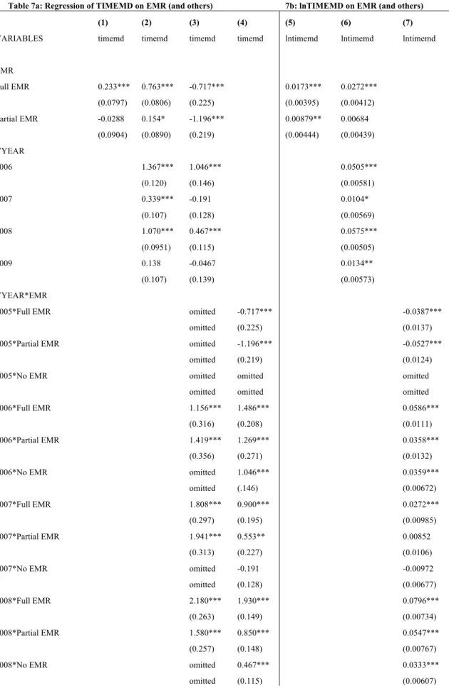
physician/physician group). I also use a model that includes an interaction term between year of visit and type of EMR system used. Each interaction coefficient may be compared to a visit in
2005 where no EMR system was in place. All cases in Table 7 are modeled using the OLS functional form with robustness checks. It is important to note that while the results from the
OLS models are significant, there is reason to believe that those results may be biased due to endogeneity in the EMR variable.
In order to correct for the endogeneity in the EMR variable, instrumental variables and a
two stage least squares regression is used. The first stage of the 2SLS models physician
characteristics that make it more likely that physician to adopt EMR systems. This comes from
the latent model that describes a physician’s choice to adopt EMR systems. The model is as follows:
EMRht = β0 +β1Wht+ β2Tht + θt +εht
variables for year 2005-2009 (with 2005 as the base), and ε is the error term. Physician
characteristics include physician specialty, region, practice ownership status, and type of practice
(these are the same variables used in the model for time). Technology characteristics include the type of electronic billing used (full, partial, or none) and the ability to do email consultations with patients. The probability of using an EMR system is modeled using the Probit model.
Even though the data will model the probability of choosing an EMR system, it will also be able to show what physician characteristics will be beneficial when that physician adopts due to the
Federal mandate and not by choice.
Finally, after computing both models, instrumental variables and a 2 stage least squares regression is used to control endogeneity in the EMR variable. My goal is to control for the
unobservable reasons that cause certain physicians to choose EMR systems, and in turn make those systems either efficient or inefficient. If the coefficient on the EMR variable changes with
the use of instruments, it can be concluded that the original results are biased (assuming that the instruments are valid). One instrument that could be used is a variable that shows the physician’s comfort level with technology. Since that particular variable is not available in the data set
electronic billing and e-mail consultations act proxies for a physician’s reasons for favoring technology.
V. Data
Statistics2. While the survey ranges from 1973-2012, I will only be looking at the years 2005-2010.The variable survey question the status of the physician’s EMR system was not asked until
2003, however that question was improperly coded for the years 2003 and 2004. The survey, which is randomized across the country, was given to physicians for a one-week period. During that time, the physician answers question both on his/herself and practice, and on the patients in
order to get more reliable results. While the survey is answered on a physician level, entries are reported on the patient visit level. Only visits to non-federally funded “office based, patient
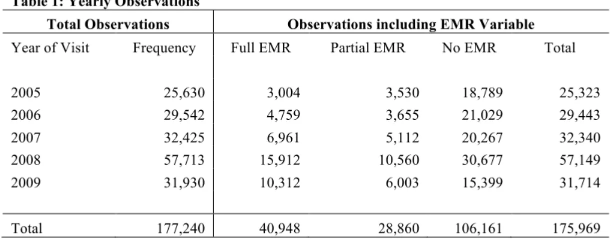
care” are included in the survey. Each year of the data is collected independently from all other years. The data is in the pooled cross sectional format. While there are a total of 177,240
observations in the sample, there are only 175,969 observations for the variable EMEDREC (for
a yearly breakdown of observations, see Table 1in the appendix).
NAMCS is a well-established, reliable data set. Sample design descriptions, variable
descriptions, and the codebooks for each year provide a clear insight into how the survey was conducted and how each variable should be used. The NAMCS data also provides many strengths in comparison to other surveys. First and foremost, data containing information on
electronic medical records is extremely hard to come by since EMR systems have only been introduced in recent years and many private practices and hospitals are not required to release
data. It is valuable in that it offers a large number of observations each year, and that the same questions are asked year after year. While panel data would have been much more ideal to follow how physicians individually adjust to EMR adoption over time, the pooled cross section
still allows researchers to study the overall change over time.
While this seems to be the best data source available at the time, it does not come without some challenges. There are no location or county codes, so it is not possible to obtain county
characteristics from other data sources. Another problem is in the fact that only non-federally funded office-based patient care facilities are surveyed. While physicians working in hospitals were not represented at all, 82.5% of the patients in the sample were seen in a private solo or
group practice. Another possible problem is with the TIME variable (time patient spent with physician). This is a discrete variable top coded at 240 minutes. The top code should not have
too much of an impact, seeing as only .04% of the time observations were top coded. I also include a model that uses lnTIME as the dependent variable, because time seems to be
distributed in the natural log form. To correct for times of 0 minutes, the variable generated is
actually ln(TIME+1). Missing values also do not cause many problems in the data set. The key independent variable, EMR, has .7% missing values. Other categorical variables either did not
have missing values, or the response “blank” was recoded and grouped with “other” in data analysis. I am looking at time as a measure of physician efficiency because cost and accuracy variables are not available in the data set. There have already been studies assessing the cost
impacts of EMR systems, however there have not been any studying better patient outcomes, i.e. more efficient visits, more accurate diagnosis, quicker recovery times, or lower mortality rates.
Because the NAMCS data does not include any information on accuracy of diagnosis, recovery times, or mortality rates, I use patient visit time as to examine EMR efficiency.
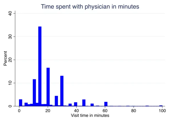
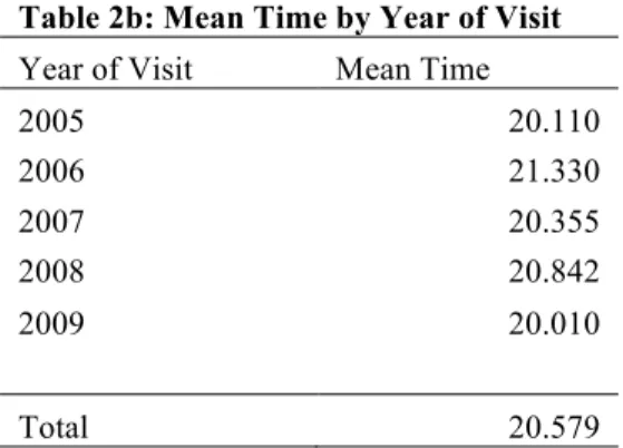
I have already touched on the fact that TIME, time the patient spent with the physician, is
the dependent variable. For the full data set, the mean time the patient spent with a physician is 20.58 minutes. That time fluctuates between 20 and 22 minutes year to year, in no specific
type of EMR system the physician is using. It is interesting to note that when only looking at type of EMR system and average time, partial EMR systems have the lowest average time a
patient spends with a physician. See Figure 1 and Table 2a-2b in the appendix for a description of TIME.
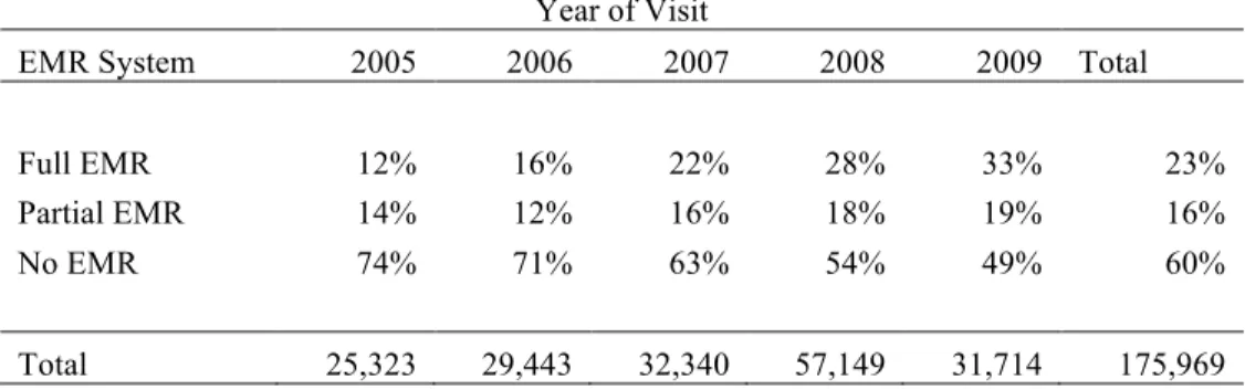
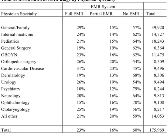
The variable EMR is the key independent variable for this study. EMR is a categorical
variable that describes the type of EMR system in place. Choices are Full EMR, Partial EMR (part electronic, part paper), or No EMR and Blank. For purposes of my analysis, I replaced all
“Blank” answers as missing values. Each year the percentage of physicians using EMR systems in some capacity increases. It is also interesting to look at the breakdown of EMR usage by physician specialty. While Cardiologists have the highest percent of EMR usage at 55% usage,
psychiatrists only have 21% usage. Those results make sense, seeing as Cardiology involves many high-tech tests and imaging while psychiatry does not. See Tables 1, 3 and 4 in the
appendix for a better description of the EMR variable. A description of other variables used in the analysis along with a set of summary statistics is included in the appendix in tables 5 and 6.
VI. Results and Findings
After running the regressions, one thing is clear from the beginning; EMR systems have a
significant impact on the length of time a patient spends with a physician. Although the results from the OLS models show a that EMR systems have a significant impact on patient visit time,
the results are likely biased due to endogeneity in the EMR variable. When looking at the baseline model for the impact of EMR systems on the natural log of patient visit time, full systems increase the time the patient spent with the physician by almost 3% in comparison to no
yearly time changes (later years were not more efficient as one might expect). Also as expected, in comparison to patients being seen for a new condition, pre/post surgery patients’ visits times
are 11% shorter and patients on routine visits for a chronic condition had 5% shorter visit times. That result could show that while EMR systems are not necessarily efficient for first time
patients, they do become efficient for that particular patient after his/her original visit. Once the
interaction term was introduced, visits in 2005 with full EMR systems are shown to be the most efficient. This result is very surprising and could be due to the endogeneity in the EMR variable.
When compared to the base cell, 2005 and no EMR system, all other years and combinations are less efficient. The magnitude of inefficiency (in comparison to the base cell) did not follow a pattern for years 2006-2009. These results can all be found in Table 7a-b in the appendix.
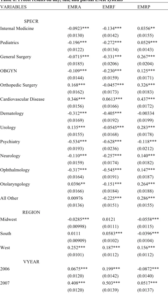
In order to model the physician’s decisions to choose EMR systems, I use three separate probit models (Results can be found in Table 8). I use three different dependent variables in the
probit models; the first is EMRA (=1 if full system or partial system is in place), followed by EMRF (full system) and EMRP (partial system). In comparison to 2005, the probability to adopt any system or a full system increased each year, however there were not yearly increases for
partial systems. If office owners felt as if they would be required to have full EMR systems in the near future, it is likely they would not adopt partial systems; instead you would expect them
to go ahead and adopt full systems. Furthermore, in comparison to family/general physicians, cardiologists were the most likely to adopt EMR systems in every model and psychiatrists were the least likely to adopt in each model. Both of these results validate the theory that physicians
whose jobs require analyzing more quantitative data (such as numerical test results or imagining) are more likely to adopt EMR systems versus those whose jobs require a qualitative analysis of
adopting full EMRs is the lowest. Those physician’s may feel as if they are already running their practice efficiently and therefore do not want to deal with the hassle of adopting EMR systems.
As far as region is concerned, offices in the West are the most likely to adopt EMRs in every model. I believe that could be partly due to the fact that Silicon Valley is located in the West, and the West in general seems a step ahead of the rest of the country in terms of technology
usage. Finally, offices with electronic billing methods and email consultations were more likely to adopt EMR systems across the board. Those two results are important because they hint at
physicians’ preferences for technology and that there may be heterogeneous effects for EMR systems. Physicians who are comfortable with or enjoy using technology should be more likely to adopt EMR systems. Moreover, those same physicians should be more efficient when using
EMR systems versus physicians who are not comfortable with technology.
The two stage least square model uses electronic billing and e-mail consultations as
instruments to capture some of the endogeneity in the EMR variable. Electronic billing and email consultations act as proxies for some other unobserved variable that causes physicians to favor technology. In order to use these instruments, it needs to be assumed that there is no
correlation between a physician’s technology preferences and the type of patients the physicians sees. Electronic billing is a categorical variable where 1=full electronic billing system in place,
2= partial electronic billing system in place, and 3= no electronic billing system. The sample is made up of 67% full systems, 24% partial, and 9% no electronic billing system. E-mail
consultations is a dummy variable where 1=yes the physician uses e-mail to communicate with
patients. Only 7% of physicians surveyed communicated with patients via email. In the 2SLS model, I use the variable EMRA again (=1 if either full or partial EMR systems are in place) as
variable. Prior to using the 2SLS model, the presence of any type of EMR system increased visit time by about 2%. After running the 2SLS model with EBILLREC (electronic billing) and
ECONR (e-mail consultations) as instruments for EMRA, the presence of any type of EMR system actually decreased visit time by 24.2%. I also ran the 2SLS model with only electronic billing as the instrument for the EMR variable, and then again using only e-mail consultations as
the only instrument. Both of those regressions show that once again, there is endogeneity in the error term. All results from the 2SLS model can be found in the appendix in Table 9. When
electronic billing is the only instrument used, any form of EMR system decreases patient visit time by 23.9%. Additionally, when e-mail consultations is the only instrument used, any form of EMR system decreases patient visit time by 58.1%. While all of the effects of EMR systems on
time are significant in all models, it can be concluded that electronic billing status is a stronger instrument than e-mail consultations (this could be due in large part that only 7% of physicians in
the sample use e-mail consultations). It is important to note that while these instruments are good, it is possible that better instruments may be found down the road in different data sets. There might still be unobserved variables that both cause physicians to have higher patient visit
times, and to have EMR systems. It is nearly impossible to pick up all of the endogeneity in the EMR variable.
VII. Conclusions
The 2SLS results are very important in my research. Not only do they show that there is endogeneity in the EMR variable, but the results also combat previous findings that EMR
systems are inefficient (in terms of patient visit time). Through out previous research, the endogeneity in the EMR variable seems to have been overlooked. Such endogeneity may be the
visit time. Without controlling for endogeneity, a 3% increase in time makes the systems look inefficient. The biased inefficiency results are a likely reason that some professionals are
hesitant to adopt the systems. That being said, the adoption of electronic medical records is more or less inevitable because of the HITECH Act, and an overall increase in technology throughout all industries. The data shows new EMR systems were being added every year the years
2005-2009; such new systems could be part of the reason why efficiency did not increase over the years (in the OLS model or in the 2SLS model). The 2SLS regression offers up very interesting
results. When adding in electronic billing and email consultations as instruments for EMR systems, EMR systems actually decreased the time of a visit by 24.2% (this result was significant at the 1% level). Much endogeneity exists in the EMR variable. It is not EMR systems alone
that increase the time of visit, but rather other unobserved variables. Such variables could be the type of patients the physician treats or how long the system has been in place. Electronic billing
and e-mail consultations are used as instruments in my research because I think that they are the best suited instruments my data set provides.
It is important to note that when looking at the results of my research, they are all for
patient visits in office settings, not hospital settings. While it is likely that similar results would occur when studying the effects of EMR systems on hospital visit times, there are some
differences in the two visits. Office visits tend to be shorter than hospital visits since in general longer, more advanced procedures and testing takes place in a hospital setting. I hypothesize that the sign of the impact of EMR systems on time is the same for office visits as hospital visits, but
those impacts might have different magnitudes. In future studies, panel data would be most beneficial in studying the effect of adopting EMR systems on physician efficiency. Being able to
EMR systems changed (grew) over the life of the EMR system. Panel data would also remove some of the endogeneity in the EMR variable if the physicians continued to see the same type of
patients year after year. It would also be beneficial to have dependent variables other than the amount of time a patient spent with a physician to measure the social benefits of EMR systems. Such benefits could include one for the quality of care received, patient recovery time, patient
mortality rates with certain diseases, detection time of certain diseases etc. Once better data is available for the use of EMR systems, more in-depth economic analysis of the systems will be
VIII. Appendix
Table 1: Yearly Observations
Total Observations Observations including EMR Variable
Year of Visit Frequency Full EMR Partial EMR No EMR Total
2005 25,630 3,004 3,530 18,789 25,323
2006 29,542 4,759 3,655 21,029 29,443
2007 32,425 6,961 5,112 20,267 32,340
2008 57,713 15,912 10,560 30,677 57,149
2009 31,930 10,312 6,003 15,399 31,714
Total 177,240 40,948 28,860 106,161 175,969
Figure 1: Distribution of time
0
10
20
30
40
Pe
rce
n
t
0 20 40 60 80 100
Visit time in minutes
Time spent with physician in minutes
All data from NAMCS 2005-2010 data sets N=177,240
This figure shows how the time a patient spent with a physician is distributed. In the graph, the time variable is top coded at 100 minutes.
Table 2a: Mean Time by EMR System Table 2b: Mean Time by Year of Visit EMR System Mean Time Year of Visit Mean Time
Full EMR 20.758 2005 20.110
Partial EMR 20.496 2006 21.330
No EMR 20.525 2007 20.355
2008 20.842
Total 20.579 2009 20.010
Total 20.579
Table 3: Break down of EMR System Type by Year of Visit Year of Visit
EMR System 2005 2006 2007 2008 2009 Total
Full EMR 12% 16% 22% 28% 33% 23%
Partial EMR 14% 12% 16% 18% 19% 16%
No EMR 74% 71% 63% 54% 49% 60%
Total 25,323 29,443 32,340 57,149 31,714 175,969
Table 4: Break down of EMR usage by Physician Specialty EMR System
Physician Specialty Full EMR Partial EMR No EMR Total
General/Family 29% 15% 57% 39,920
Internal medicine 24% 14% 62% 14,727
Pediatrics 21% 15% 64% 18,243
General Surgery 19% 19% 62% 6,364
OBGYN 23% 16% 62% 11,475
Orthopedic surgery 26% 20% 54% 8,509
Cardiovascular Disease 31% 23% 45% 9,496
Dermatology 19% 13% 68% 8,306
Urology 26% 19% 54% 9,494
Psychiatry 10% 12% 79% 8,244
Neurology 20% 16% 64% 9,813
Ophthalmology 15% 16% 70% 9,108
Otolaryngology 25% 19% 56% 8,217
All other 21% 20% 59% 14,053
Total 23% 16% 60% 175,969
Table 5: Variable Descriptions
Short Name Variable Name Long Definition TIME Amount of time patient
spent with physician
TIME is a discrete variable measured in minutes that takes on values 0-240. Time is recorded at the end of the visit by the physician.
EMR Type of EMR system used by physician
EMR is a categorical variable that contains values 1=Full EMR System, 2=Partial EMR System, 3=No EMR System
VYEAR Year of Visit VYEAR is a discrete variable that records the year the visit takes place. It ranges from 2005-2009
RACER Race of patient RACER is a categorical variable that records the race of the patient. 1=White, 2=Black, 3=Other.
REGION Geographical region the visit took place
REGION is a categorical variable that records the region of country where the visit took place. 1=Northeast, 2=Midwest, 3=South, 4=West. States included in the survey by region are as follows; Northeast: Connecticut, Maine, Massachusetts, New Hampshire, New Jersey, New York, Pennsylvania, Rhode Island, Vermont, Midwest: Illinois, Indiana, Iowa, Kansas, Michigan, Minnesota, Missouri, Nebraska, North Dakota, Ohio, South Dakota, Wisconsin, South: Alabama, Arkansas, Delaware, District of Columbia, Florida, Georgia, Kentucky, Louisiana, Maryland, Mississippi, North Carolina,
Oklahoma, South Carolina, Tennessee, Texas, Virginia, West Virginia, West: Arizona, California, Colorado, Idaho, Montana, Nevada, New Mexico, Oregon, Utah, Washington, Wyoming, Alaska, Hawaii.
MAJOR Major reason for the patient's visit
MAJOR is a categorical variable where 1=New Problem, 2=Chronic Problem, Routine, 3=Chronic Problem, Flare-Up, 4=Pre/Post Surgery, 5=Preventative Care (this includes yearly checkups and pre-natal care)
PAYTYPE0 Patient's payment method for the visit
PAYTYPE0 is a categorical variable that describes how the patient paid for the physician's services where 1=Private Insurance, 2=Medicare, 3=Medicaid, 4=Other, 5=Unknown RETYPOFF Type of office setting RETYPOFF is a categorical variable that describes the type of
office the physician is operating in where 1= Private Solo/Group Practice, 2= Free Standing Urgent Care, 3= Community Health Center, 4=Other
OWNS Ownership Status of the physician office
OWNS is a categorical variable that measures the ownership status of the practice where the visit took place.
1=Physician/Physician Group, 2=Health Maintenance Organization (HMO), 3=Community Health Center, 4=Medical/Academic Center, 5=Other
AGE Age of patient AGE is a discrete variable ranging from 0-100 that describes the age of the patient. Any patients falling under the age of 1 have an age recorded as 0. Any patients 100 or older have an age recorded as 100.
Table 6: Summary Statistics
Variable Mean
Std.
Dev. Min Max
Time 20.57695 13.81688 0 240
Age 45.90116 24.66199 0 100
Year of Visit 2007.23 1.317808 2005 2009
Variable Percent Variable Percent
Race Practice Ownership Status
White 83.23 Physician/Physician Group 76.95
Black 11.3 HMO 2.17
Other 5.46 Community Health Center 9.94
Medical/Academic Center 2.14
Reason for Visit Other 8.79
New Problem 32.28
Chronic, Routine 33.49 Physician Specialty
Chronic, Flare-Up 8.85 General/Family 22.72 Pre/Post-Surgery 7.56 Internal Medicine 8.31
Preventative Care 17.81 Pediatrics 10.42
General Surgery 3.65
Patient Payment Method OBGYN 6.55
Private Insurance 49.82 Orthopedic Surgery 4.87 Medicare 23.38 Cardiovascular Disease 5.37
Medicaid 13.17 Dermatology 4.7
Other 9.55 Urology 5.4
Unknown 4.09 Psychiatry 4.66
Neurology 5.52
Type of Office Setting Ophthalmology 5.19 Private Solo/Group Practice 82.57 Otolaryngology 4.7 Free Standing Urgent Care 3.97 All Other 7.94 Community Health Center 10.17
Other 3.29
Table 7a: Regression of TIMEMD on EMR (and others) 7b: lnTIMEMD on EMR (and others)
(1) (2) (3) (4) (5) (6) (7)
VARIABLES timemd timemd timemd timemd lntimemd lntimemd lntimemd
EMR
Full EMR 0.233*** 0.763*** -0.717*** 0.0173*** 0.0272*** (0.0797) (0.0806) (0.225) (0.00395) (0.00412)
Partial EMR -0.0288 0.154* -1.196*** 0.00879** 0.00684 (0.0904) (0.0890) (0.219) (0.00444) (0.00439)
VYEAR
2006 1.367*** 1.046*** 0.0505***
(0.120) (0.146) (0.00581)
2007 0.339*** -0.191 0.0104*
(0.107) (0.128) (0.00569)
2008 1.070*** 0.467*** 0.0575***
(0.0951) (0.115) (0.00505)
2009 0.138 -0.0467 0.0134**
(0.107) (0.139) (0.00573)
VYEAR*EMR
2005*Full EMR omitted -0.717*** -0.0387***
omitted (0.225) (0.0137)
2005*Partial EMR omitted -1.196*** -0.0527***
omitted (0.219) (0.0124)
2005*No EMR omitted omitted omitted
omitted omitted omitted
2006*Full EMR 1.156*** 1.486*** 0.0586***
(0.316) (0.208) (0.0111)
2006*Partial EMR 1.419*** 1.269*** 0.0358***
(0.356) (0.271) (0.0132)
2006*No EMR omitted 1.046*** 0.0359***
omitted (.146) (0.00672)
2007*Full EMR 1.808*** 0.900*** 0.0272***
(0.297) (0.195) (0.00985)
2007*Partial EMR 1.941*** 0.553** 0.00852
(0.313) (0.227) (0.0106)
2007*No EMR omitted -0.191 -0.00972
omitted (0.128) (0.00677)
2008*Full EMR 2.180*** 1.930*** 0.0796***
(0.263) (0.149) (0.00734)
2008*Partial EMR 1.580*** 0.850*** 0.0547***
(0.257) (0.148) (0.00767)
2008*No EMR omitted 0.467*** 0.0333***
2009*Full EMR
(1) (2) (3)
0.930*** (4) 0.166
(5) (6) (7)
0.0191**
(0.270) (0.142) (0.00797)
2009*Partial EMR 1.330*** 0.0874 0.0148
(0.296) (0.193) (0.00955)
209*No EMR omitted -0.0467 -0.00349
omitted (0.139) (0.00728)
REGION
Midwest -1.788*** -1.762*** -1.762*** -0.0759*** -0.0748***
(0.0971) (0.0971) (0.0971) (0.00477) (0.00477) South -0.823*** -0.811*** -0.811*** -0.0433*** -0.0427***
(0.0940) (0.0940) (0.0940) (0.00444) (0.00444)
West 0.115 0.133 0.133 0.00384 0.00495
(0.104) (0.103) (0.103) (0.00488) (0.00488) RACER
Black -0.176* -0.169* -0.169* -0.0128** -0.0126**
(0.0999) (0.0998) (0.0998) (0.00527) (0.00527)
Other 0.132 0.129 0.129 0.0290*** 0.0291***
(0.131) (0.131) (0.131) (0.00655) (0.00656)
SPECR
Internal Medicine 1.435*** 1.430*** 1.430*** 0.0706*** 0.0706***
(0.116) (0.117) (0.117) (0.00640) (0.00640) Pediatrics -0.860*** -0.834*** -0.834*** -0.0176** -0.0167**
(0.123) (0.122) (0.122) (0.00686) (0.00686) General Surgery 1.413*** 1.432*** 1.432*** 0.0873*** 0.0878***
(0.189) (0.189) (0.189) (0.00853) (0.00854) OBGYN -1.021*** -1.011*** -1.011*** -0.0283*** -0.0284***
(0.125) (0.125) (0.125) (0.00761) (0.00762) Orthopedic Surgery -0.421*** -0.433*** -0.433*** -0.0123 -0.0127
(0.152) (0.152) (0.152) (0.00799) (0.00799) Cardiovascular Disease 0.831*** 0.840*** 0.840*** 0.0562*** 0.0565***
(0.137) (0.137) (0.137) (0.00787) (0.00787) Dernatology -1.363*** -1.350*** -1.350*** -0.0855*** -0.0854***
(0.172) (0.172) (0.172) (0.00790) (0.00789)
Urology 0.623*** 0.630*** 0.630*** 0.0417*** 0.0419***
(0.145) (0.145) (0.145) (0.00761) (0.00763)
Psychiatry 15.42*** 15.41*** 15.41*** 0.549*** 0.549***
(0.212) (0.212) (0.212) (0.0100) (0.0100)
Neurology 9.655*** 9.682*** 9.682*** 0.376*** 0.377***
(0.198) (0.198) (0.198) (0.00809) (0.00812)
Ophthalmology 0.0250 0.0555 0.0555 0.0240*** 0.0249***
Otolaryngology
(1) (2)
0.448*** (3) 0.473***
(4) 0.473***
(5) (6)
0.0515*** (7) 0.0521*** (0.135) (0.135) (0.135) (0.00765) (0.00764)
All Other 5.511*** 5.511*** 5.511*** 0.180*** 0.180***
(0.184) (0.184) (0.184) (0.00763) (0.00763)
PAYTYPE0
Medicare -0.583*** -0.579*** -0.579*** -0.0288*** -0.0289***
(0.0975) (0.0975) (0.0975) (0.00474) (0.00474) Medicaid -0.443*** -0.451*** -0.451*** -0.0272*** -0.0276***
(0.0976) (0.0977) (0.0977) (0.00533) (0.00533)
Other 1.416*** 1.417*** 1.417*** 0.0148** 0.0147**
(0.131) (0.131) (0.131) (0.00639) (0.00639)
Unknown 1.357*** 1.332*** 1.332*** 0.00202 0.00128
(0.246) (0.246) (0.246) (0.00889) (0.00890) MAJOR
Chronic, Routine -1.050*** -1.049*** -1.049*** -0.0449*** -0.0448*** (0.0868) (0.0868) (0.0868) (0.00421) (0.00421)
Chronic, Flare-Up 1.000*** 0.996*** 0.996*** 0.0600*** 0.0600*** (0.125) (0.125) (0.125) (0.00565) (0.00565)
Pre/Post Surgery -1.994*** -2.005*** -2.005*** -0.105*** -0.106*** (0.144) (0.144) (0.144) (0.00658) (0.00658)
Preventative Care 0.726*** 0.722*** 0.722*** 0.0155*** 0.0154*** (0.0903) (0.0903) (0.0903) (0.00517) (0.00517)
OWNS
Health Maintenance Org. 0.776*** 0.784*** 0.784*** 0.0650*** 0.0663***
(0.217) (0.217) (0.217) (0.0107) (0.0107) Community Health Center -0.188* -0.170 -0.170 0.0449*** 0.0457***
(0.108) (0.108) (0.108) (0.00601) (0.00601) Medical/Academic Center 0.311 0.340 0.340 0.0489*** 0.0495***
(0.225) (0.225) (0.225) (0.00974) (0.00975)
Other -0.0868 -0.0754 -0.0754 0.0115* 0.0119**
(0.119) (0.119) (0.119) (0.00593) (0.00593)
AGE 0.0229*** 0.0229*** 0.0229*** 0.00137*** 0.00137***
(0.00206) (0.00206) (0.00206) (0.000101) (0.000101) Constant 20.52*** 17.90*** 18.24*** 18.24*** 2.886*** 2.770*** 2.785***
(0.0432) (0.146) (0.152) (0.152) (0.00210) (0.00789) (0.00818)
Observations 175,969 172,791 172,791 172,791 175,969 172,791 172,791 R-squared 0.0001 0.093 0.094 0.094 0.000 0.054 0.054
All data from NAMCS 2005-2010 data sets N=172,791
Robust standard errors in parentheses *** p<0.01, ** p<0.05, * p<0.1
Base variables: EMEDREC-No EMR system, REGION-Northeast, RACER-White, SPECR- General/Family, PAYTYPE0- Private insurance, MAJOR-New health problem, OWNS- Physician/Physician Group
Table 8: Probit results on any, full, and partial EMR systems
VARIABLES EMRA EMRF EMRP
SPECR
Internal Medicine -0.0923*** -0.134*** 0.0356** (0.0130) (0.0142) (0.0155) Pediatrics -0.196*** -0.272*** 0.0529***
(0.0122) (0.0134) (0.0143) General Surgery -0.0715*** -0.331*** 0.267***
(0.0185) (0.0206) (0.0204)
OBGYN -0.109*** -0.230*** 0.125***
(0.0144) (0.0159) (0.0171) Orthopedic Surgery 0.168*** -0.0457*** 0.326***
(0.0162) (0.0173) (0.0183) Cardiovascular Disease 0.346*** 0.0613*** 0.437***
(0.0156) (0.0166) (0.0172) Dernatology -0.312*** -0.405*** -0.00334 (0.0169) (0.0192) (0.0199) Urology 0.135*** -0.0545*** 0.283***
(0.0155) (0.0168) (0.0178) Psychiatry -0.534*** -0.628*** -0.118***
(0.0193) (0.0236) (0.0212) Neurology -0.110*** -0.257*** 0.140***
(0.0159) (0.0174) (0.0182) Ophthalmology -0.317*** -0.545*** 0.147***
(0.0164) (0.0191) (0.0187) Otolaryngology 0.0396** -0.151*** 0.264***
(0.0166) (0.0184) (0.0188) All Other 0.00976 -0.225*** 0.286***
(0.0136) (0.0151) (0.0155) REGION
Midwest -0.0285*** 0.0121 -0.0558*** (0.00998) (0.0111) (0.0115)
South 0.0111 0.0583*** -0.0396***
(0.00909) (0.0102) (0.0104)
West 0.252*** 0.187*** 0.156***
(0.0101) (0.0112) (0.0112) VYEAR
2006 0.0675*** 0.199*** -0.0872***
(0.0120) (0.0142) (0.0140)
2007 0.408*** 0.503*** 0.0517***
(1) (2) (3)
2008 0.662*** 0.735*** 0.155***
(0.0108) (0.0125) (0.0122)
2009 0.809*** 0.888*** 0.173***
(0.0119) (0.0135) (0.0133) OWNS
Health Maintenance Org. 1.109*** 1.087*** -0.218*** (0.0342) (0.0302) (0.0330) Community Health Center 0.389*** 0.193*** 0.356***
(0.0378) (0.0328) (0.0447) Medical/Academic Center 0.0294 0.116*** -0.0877***
(0.0235) (0.0251) (0.0281)
Other 0.409*** 0.328*** 0.211***
(0.0119) (0.0123) (0.0135) RETYPOFF
Free Standing Urgent Care 0.213*** 0.0969*** 0.187*** (0.0169) (0.0180) (0.0186) Community Health Center -0.328*** -0.294*** -0.126***
(0.0375) (0.0324) (0.0449)
Other 0.671*** 0.382*** 0.356***
(0.0247) (0.0239) (0.0253) EBILLREC
Full e-billing 0.806*** 0.919*** 0.178*** (0.0133) (0.0164) (0.0148) Partial e-billing 0.501*** 0.310*** 0.400***
(0.0141) (0.0176) (0.0154) ECONR
E-Mail Consults -0.0122*** -0.0286*** 0.0225*** (0.00203) (0.00214) (0.00251) Constant -1.483*** -1.981*** -1.487***
(0.0183) (0.0218) (0.0205)
Observations 168,251 168,251 168,251
All data from NAMCS 2005-2010 data sets N=163,961
Robust standard errors in parentheses *** p<0.01, ** p<0.05, * p<0.1
Base variables: REGION-Northeast, RACER-White, SPECR- General/Family, OWNS- Physician/Physician Group, RETYPOFF- Private Solo/Group Practice, No electronic billing
Table 9: IV 2SLS with EMR as instrumented variable
OLS IV with 2SLS
(1) (2) (3) (4)
VARIABLES ln(time) ln(time) ln(time) ln(time)
EMRA 0.0169*** -0.242*** -0.239*** -0.581*** (0.00346) (0.0208) (0.0208) (0.224) VYEAR
2006 0.0519*** 0.0573*** 0.0572*** 0.0643*** (0.00582) (0.00588) (0.00588) (0.00776) 2007 0.00813 0.0355*** 0.0352*** 0.0714***
(0.00576) (0.00622) (0.00621) (0.0246) 2008 0.0588*** 0.108*** 0.108*** 0.173***
(0.00509) (0.00637) (0.00638) (0.0431) 2009 0.0132** 0.0773*** 0.0766*** 0.161***
(0.00576) (0.00773) (0.00774) (0.0558) REGION
Midwest -0.0774*** -0.0817*** -0.0817*** -0.0874*** (0.00483) (0.00491) (0.00491) (0.00653) South -0.0461*** -0.0424*** -0.0424*** -0.0375***
(0.00448) (0.00457) (0.00457) (0.00575) West 0.00409 0.0254*** 0.0252*** 0.0533***
(0.00497) (0.00534) (0.00534) (0.0190) RACE
Black -0.0159*** -0.0252*** -0.0251*** -0.0373*** (0.00535) (0.00548) (0.00548) (0.00984) Other 0.0275*** 0.0249*** 0.0249*** 0.0215***
(0.00677) (0.00691) (0.00691) (0.00778) MAJOR
Chronic, Routine -0.0442*** -0.0475*** -0.0475*** -0.0519*** (0.00428) (0.00437) (0.00437) (0.00553) Chronic, Flare-Up 0.0610*** 0.0586*** 0.0586*** 0.0553***
(0.00573) (0.00586) (0.00585) (0.00666) Pre/Post Surgery -0.104*** -0.102*** -0.102*** -0.0992***
(0.00669) (0.00680) (0.00679) (0.00752) Preventative Care 0.0175*** 0.0200*** 0.0199*** 0.0232***
(0.00525) (0.00534) (0.00533) (0.00608) SPECR
Internal Medicine 0.0737*** 0.0657*** 0.0658*** 0.0552*** (0.00648) (0.00667) (0.00667) (0.0100) Pediatrics -0.0226*** -0.0387*** -0.0385*** -0.0598***
(1) (2) (3) (4)
General Surgery 0.0826*** 0.0768*** 0.0769*** 0.0692*** (0.00862) (0.00875) (0.00874) (0.0106) OBGYN -0.0350*** -0.0467*** -0.0466*** -0.0620***
(0.00778) (0.00795) (0.00794) (0.0132) Orthopedic Surgery -0.0146* 0.00349 0.00330 0.0272
(0.00806) (0.00829) (0.00828) (0.0180) Cardiovascular Disease 0.0549*** 0.0938*** 0.0934*** 0.145***
(0.00796) (0.00866) (0.00866) (0.0348) Dermatology -0.0882*** -0.115*** -0.115*** -0.150***
(0.00799) (0.00843) (0.00842) (0.0248) Urology 0.0375*** 0.0533*** 0.0532*** 0.0740***
(0.00774) (0.00792) (0.00791) (0.0163) Psychiatry 0.545*** 0.497*** 0.497*** 0.433***
(0.0102) (0.0109) (0.0109) (0.0431) Neurology 0.375*** 0.365*** 0.365*** 0.352***
(0.00824) (0.00847) (0.00847) (0.0125) Ophthalmology 0.0236*** -0.00239 -0.00211 -0.0365
(0.00727) (0.00772) (0.00772) (0.0241) Otolaryngology 0.0462*** 0.0544*** 0.0543*** 0.0652***
(0.00788) (0.00799) (0.00799) (0.0111) All Other 0.179*** 0.180*** 0.180*** 0.181***
(0.00773) (0.00785) (0.00785) (0.00833) PAYTYPE0
Medicare -0.0303*** -0.0331*** -0.0331*** -0.0369*** (0.00482) (0.00491) (0.00491) (0.00579) Medicaid -0.0285*** -0.0361*** -0.0360*** -0.0460***
(0.00540) (0.00553) (0.00553) (0.00883) Other 0.0166** 0.00707 0.00717 -0.00547
(0.00651) (0.00662) (0.00662) (0.0109) Unknown 0.00186 0.0344*** 0.0341*** 0.0772***
(0.00911) (0.00955) (0.00955) (0.0298) OWNS
Health Maintenance Org. 0.0742*** 0.192*** 0.191*** 0.347*** (0.0115) (0.0149) (0.0149) (0.103) Community Health Center 0.0440*** 0.0513*** 0.0512*** 0.0608***
(0.00614) (0.00626) (0.00626) (0.00914) Medical/Academic Center 0.0459*** 0.0616*** 0.0615*** 0.0823***
(0.0101) (0.0107) (0.0106) (0.0178) Other 0.00651 0.0519*** 0.0514*** 0.111***
(1) (2) (3) (4)
AGE 0.00136*** 0.00137*** 0.00137*** 0.00138*** (0.000102) (0.000104) (0.000104) (0.000112) Constant 2.774*** 2.837*** 2.836*** 2.920***
(0.00796) (0.00941) (0.00941) (0.0556)
Observations 168,251 168,251 168,251 168,251
R-squared 0.055 0.023 0.024
All data from NAMCS 2005-2010 data sets N=168,251
Robust standard errors in parentheses *** p<0.01, ** p<0.05, * p<0.1
Base variables: REGION-Northeast, RACER-White, SPECR- General/Family, PAYTYPE0- Private insurance, MAJOR-New health problem, OWNS- Physician/Physician Group
The variable EMRA is a dummy variable =1 if EMR= 1 or 2 (either a full or partial EMR system is in place) Model 1 is an OLS model of ln(TIME+1) on EMRA and a set of controls
Model 2 is an IV 2SLS where instrumented: EMRA, instruments: year, race, region, speciality, major, payment, ownership, age, billing, and e-mail consultation variables
IX. References
Baker, Laurence C., Kate Bundorf, and Daniel Kessler. "Expanding Patients' Property Rights in Their Medical Records (Working Paper No. 20565)." (2014): Retrieved from National Bureau of Economics. Web. <http://www.nber.org/papers/w20565>.
Brunt, Christopher S., and John R. Bowblis. "Health IT Adoption, Productivity and Quality in Primary Care." Applied Economics 46.15 (2014): 1716-1727.
Christensen, Michael C., and Dahlia Remler. "Information and Communications Technology in Chronic Disease Care: Why Is Adoption so Slow and Is Slower Better? (Working Paper No. 13078)." (2007): Retrieved from National Bureau of Economic Research. Web. <http://www.nber.org/papers/w13078>.
Dranove, David, Chris Forman, Avi Goldfarb, and Shane Greenstein. "The Trillion Dollar Conundrum: Complementarities and Health Information Technology." American Economic Journal: Economic Policy 6.4 (2014): 239-70. Web.
http://dx.doi.org/10.1257/pol.6.4.239
Hoggle, Lindsey Blevins, Martin M. Yadrick, and Elaine J. Ayres. "A Decade of Work Coming Together: Nutrition Care, Electronic Health Records, and the HITECH Act." National Center for Biotechnology Information. U.S. National Library of Medicine, 01 Nov. 2011. Web. 19 Oct. 2014.