Sharif University of Technology
Scientia IranicaTransactions E: Industrial Engineering http://scientiairanica.sharif.edu
Benders decomposition algorithm for robust aggregate
production planning considering pricing decisions in
competitive environment: A case study
A. Aazami and M. Saidi-Mehrabad
Department of Industrial Engineering, Iran University of Science and Technology, University Ave., Narmak, Tehran, P.O. Box 1684613114, Iran.
Received 13 November 2017; received in revised form 12 September 2018; accepted 13 October 2018
KEYWORDS Bi-level aggregate production planning; Robust optimization; Competitive
condition; Pricing; Benders decomposition.
Abstract.In operations research, bi-level programming is a mathematical modeling which has another optimization problem as a constraint. In the present research, regarding the current intense competition among large manufacturing companies for achieving a greater market share, a bi-level robust optimization model is developed as a leader-follower problem using Stackelberg game in the eld of Aggregate Production Planning (APP). The leader company with higher inuence intended to produce new products, which could replace the existing products. The follower companies, as rivals, were also seeking more sales, but they did not have the intention and ability to produce such new products. The price of the new products was determined by the presented elasticity relations between uncertain demand and price. After linearization, using the KKT conditions, the bi-level robust model was transformed into an ordinary uni-level model. Due to the NP-hard nature of the problem, Benders Decomposition Algorithm (BDA) was proposed for overcoming the computational complexities in large scale. Finally, using the real data of Sarvestan Sepahan Co as a leader company, the validity of the developed model as well as eciency and convergence of the BDA was investigated. The computational results clearly showed the eciency and eectiveness of the proposed BDA.
© 2019 Sharif University of Technology. All rights reserved.
1. Introduction
Today, globalization of economy, rapid changes in technology, and dierent behaviors of the customers looking for more suitable and cheaper products have led to fundamental changes in the nature of market competition [1,2]. These factors, along with the advent of e-commerce, have resulted in a competition among large manufacturing companies for achieving a greater
*. Corresponding author. Tel./Fax: +98 21 73225025 E-mail addresses: a [email protected] (A. Aazami); [email protected] (M. Saidi-Mehrabad)
doi: 10.24200/sci.2018.5563.1346
market share [1-5]. As an example of such competition, two hardware manufacturers, namely HTC and Nokia, are competing for more sales in the market [1]. In such a situation, some questions may come to mind such as \which company will win the competition?" and \what market share will be achieved by the winner company [6]?" The present study aims to answer such questions and simply model the competition between a manufacturing company, which has a higher selling power and popularity in market as a leader, and others. It is of a great importance and revenue to the leader to consider the competition in its APP and pricing decisions as a bi-level model.
As one of the most important problems in pro-duction systems, especially in current competitive
mar-kets, production planning aims at coordinating the production activities and providing an eective plan that optimizes objectives of the companies. In fact, production planning is a decision-making process of allocating resources to the production activities in a cost-eective manner that makes it possible for the manufacturer to be the winner of the competitive market [7]. APP, as a special production planning, comprises the simultaneous determination of produc-tion, inventory, and employment levels as well as other important production variables of a company during a nite planning horizon. Usually, the planning horizon of APP ranges from 6 months to one year. Assuming the production capacity constraint, the ob-jective of the APP is normally to minimize the total costs while meeting the non-constant and uctuating demand [8].
In the present research, the main competition is between the leader company, with a higher selling power and popularity, and the follower companies. These companies are independent and seek a greater market share. In fact, the competition is on the amount of sales and price of products. It should be noted that in the developed model, the focus is on the leader in that its decisions aect the decisions of the followers due to its higher popularity. This type of competition is modeled using a Bi-level Linear Programming (BLP) [9]. After linearization, using the KKT conditions, the bi-level APP model is trans-formed into an ordinary uni-level one. By solving the developed model, in addition to the APP decisions and the amounts of sales of the leader and the follower, the price of products is determined using elasticity relations.
Compared to the existing literature, the main contributions of the present study can be enumerated in 3 aspects. The rst one is that we consider the competition between a manufacturer company with its corresponding Supply Chain (SC) and other manu-facturer companies with their corresponding SCs in a competitive market. The main competitive factor is the selling price, which is determined using the proposed elasticity relations between the demand and price under pricing decisions. We utilize a leader-follower bi-level programming approach using the concept of Stackelberg game for developing the competitive APP model. To the best of our knowledge, there is no modelling eort that considers this kind of competition in the APP problems. The second one is that we address the inherent uncertainty of the parameters of the problem, especially market demand, which is controlled using multiple scenarios. In fact, we solve the uncertainty using a robust optimization method introduced by Mulvey et al. [10], which has not been used by researchers in the literature for the competitive APP problem. Considering the inherent uncertainty
makes the modeling of problems much closer to the real conditions. According to the research of Makui et al. [7], the APP problems are among the strongly NP-hard ones and the use of meta-heuristic methods for solving such problems would not guarantee obtaining accurate and global optimal solutions. Consequently, it can be claimed that the developed model is NP-hard and an ecient algorithm is needed to overcome its computational complexity. Therefore, as the third contribution, the powerful Benders Decomposition Al-gorithm (BDA) is proposed to solve the developed NP-hard model in large scale. We also study a real-life case from Sarvestan Sepahan Co., as a leader in the competitive market, in order to indicate applicability of the developed model and BDA to the real-world cases of APP.
The rest of the paper is organized as follows. Section 2 provides a review of the literature on APP, production planning, and the BLP problem in com-petitive market environment as well as the pricing problem. In Section 3, the mathematical model of bi-level APP in competitive environment is developed in the presence of uncertainty. Section 4 presents the proposed BDA for solving the developed model in large dimensions. In Section 5, performance and eciency of the developed model are tested using a set of data of a school notebook manufacturing company in Isfahan, Sarvestan Sepahan Co. Finally, the last section provides conclusion as well as some suggestions for future studies.
2. Literature review
The intense competition in competitive market has compelled the companies to satisfy the demand of customers with high speed and quality [11]. In most of the recent optimization and simulation models, it has been attempted to consider the existing competition in the market. Thus, it is very important to model the competition and solve the pricing problem to meet the demand. This section reviews the previous studies of modeling of the competitive environment for manufacturing companies (particularly the bi-level models) as well as the studies of the product pricing problems. Once a manufacturing company has no rival in the market, it will indeed be an exclusive company that obtains the whole market share. However, since there are other rivals in the market, in many cases, exclusiveness of the manufacturing company will be an unreal assumption [12].
Review of the literature is presented in the fol-lowing two sub-sections. First, the studies of BLP and pricing problems in a competitive market environment are presented. Then, some of the most important researches in the eld of production planning as well as APP will be reviewed.
2.1. Review of the literature on bi-level programming and pricing problems
In this section, we review a large and growing bodyof literature in the eld of BLP modeling with focus on the application of the BLP approach to formulating some problems such as Supply Chain Network Design (SCND), production planning, transportation, pricing, location-allocation, etc. According to our investiga-tions, the main modeling of the BLP was presented for the rst time in a study conducted by Bracken and McGill [13] in 1973, while, later, Candler and Norton [14] were the rst ones who used the name of bi-level and multi-level programming. Such problems did not attract attention of the researchers up to about 8 years later. Several researchers investigated the BLP with regard to the theory of Stackelberg game [15] and developed its mathematical formulation [16]. For further studies in this eld, the interested readers can refer to the highly valuable information in [14,16-24].
Ben-Ayed et al. [25], as the rst researchers, modeled the network design problem in the form of the BLP. They considered both the convex and concave investment functions in their formulation. Bard and Moore [26], who were pioneers in the eld of the BLP, presented the branch and bound algorithm for solving the quadratic BLP. Continuing their research, they [27] introduced a new algorithm for the discrete BLP, which began by transforming the objective function of the leader into a parametric constraint. Edmunds and Bard [28] developed an algorithm based on the branch and bound for Bi-level Non-Linear Program-ming (BNLP) problem. They helped completing the literature in this regard and their paper was among the rst studies of the BNLP. Yang [29] applied the BLP approach to the origin-destination matrix estimation problem in congested networks and presented ecient heuristic algorithms. Their approach integrated the standard least squares model and the standard network equilibrium model into one process. In 1998, Bard [23] presented optimization of the BLP problem along with all of its algorithms and applications in a book, which has been a scientic reference for the BLP problems.
Most of the previous reviewed papers were pub-lished before 2000. In the following, the literature after 2000 will be investigated. Maher et al. [30] formulated two problems in transportation network including trip matrix estimation and trac signal optimization ap-plying the BLP approach with stochastic equilibrium link for users. They proposed a solution algorithm for the two BLP problems and examined their algorithm on some networks. Moreover, Burgard et al. [31] applied the BLP modeling to chemical problems to identify gene knockout strategies for optimizing micro-bial strain. Gao et al. [32] developed a traditional BLP model for discrete network design problem and pro-posed a new solution algorithm using support function
concept to represent the relationship between improve-ment ows and new additional links. Shi et al. [33] contributed a generalized branch and bound algorithm to the literature for solving the BLP problems. The branch and bound algorithm has been the most success-ful algorithm for the BLP to overcome the complemen-tary constraints resulting from the KKT conditions.
According to our vast searches, the rst serious studies on the competition between two SCs were presented by Zhang [3]. He presented a variation inequality model to the literature on competition, in which the winning SC and its market share were determined. In 2007, Colson et al. [22] published a review paper in which they investigated many papers on bi-level optimization from both theoretical and practical aspects and presented the existing gaps in this eld. Sun et al. [34] developed a BLP model as well as a simple heuristic algorithm in order for the location of the logistics distribution centers to be determined. The upper level was to nd the optimal location and the lower determined an equilibrium demand distribution. Saharidis and Lerapetritou [9] presented a new solution method for the BLP problems based on the decompo-sition technique. Their proposed algorithm was based on the decomposition of the primary problem into a restricted master problem and multiple sub-problems using the BDA. In the eld of pricing and competition, Xiao and Yang [1] developed a competitive model of two SCs under demand uncertainty with price and service factors in order to assess the optimal decisions of chain components. Each SC included one risk-neutral supplier and one risk-averse retailer. Zhang and Rushton [12] developed a multi-site location-allocation model to select locations in competitive service sys-tems. Their presented objective function maximized utility of users with constraints on the waiting time of users and budget of owners. Zhang et al. [35] developed a BLP model for a seaport container transport network, in which the transportation companies competed on using the path with the lowest cost.
In the following, the related literature after 2010 will be reviewed. Gelareh et al. [36] designed a liner shipping hub network in a competitive environment and investigated the competition between a newcomer provider and an existing well-known operator. The newcomer maximized its market share by locating predetermined hubs in candidate ports and designing the network. Kucukaydin et al. [37] investigated the competitive facility location problem by determining the attractiveness of the follower. They formulated a BNLP model in which the leader was a new rm with a facility location problem to maximize its prot and the follower was its rival rm with existing facil-ities. Naimi Sadigh et al. [38] studied coordination of the manufacturer-retailer SC with price-dependent demand within Stackelberg game framework. They
also utilized the BLP to nd advertising expenditures, optimal equilibrium prices, and production policies. Kristianto et al. [39] presented a two-stage bi-level stochastic model for the mass production problem and considered the manufacturer as the leader and the consumer as the follower in order to model the contradictory objectives between them. They used the BDA to solve the proposed complex model and obtain an optimum solution.
In recent years, the number of studies in the literature on the application of the BLP approach by considering competition in SCs has been increasing. Rezapour and Zanjirani Farahani [40], as well-known researchers in the eld of modeling of competition, developed a new stochastic BLP model to design a competitive SC considering the two competitive factors of price and service level with foresight. They assumed that the network of the new SC was set \once for all," but further price and service level modications were possible. Rezapour et al. [41], in another research, used dynamic BLP to design an entrant SC for competition against an existing SC, where demand was elastic with respect to price and distance. They modeled the problem with the strategic facility location and ow decisions, and proposed exact and metaheuristic algorithms. Fallah et al. [6] considered the competition between two closed-loop SCs including manufactur-ers, retailmanufactur-ers, and recyclmanufactur-ers, in which the competition factors were the prices of new products and the in-centives given to consumers for taking back the used products. They studied the impact of simultaneous and Stackelberg competitions between two closed-loop SCs on their prots, demands, and returns in a non-deterministic environment. As a more related study to the previous research, Rezapour et al. [42] devel-oped a competitive closed-loop SC model using the BLP with price-dependent demands in order to design a strategic reverse network and tactical/operational
planning. They considered competitions not only
externally between two chains supplying new products but also internally in the new chain for supplying new and remanufactured products.
In more recent studies, Rashidi et al. [43] de-veloped a BLP model for the location of crosswalks in a multimodal transportation network to minimize the pedestrians' safety hazard and total transportation cost. They employed a greedy heuristic and a simulated annealing algorithm to solve the problem. Han et al. [44] presented a solution to the bi-level and tri-level programming problems using Particle Swarm Optimization (PSO) algorithm. They rst developed a novel bi-level PSO to solve general BLP problems and then, proposed a tri-level PSO for handling the tri-level programs that were more challenging than the BLPs. Saranwong and Likasiri [45] used the BLP to solve Distribution Center (DC) problem by which the
upper-and lower-levels were to minimize the transportation cost of shipping products from plants to DCs and from DCs to customers, respectively. They also presented four algorithms to obtain an optimal trade-o between the objective function values of the two levels. In the last paper we reviewed, but certainly not the latest research conducted on the BLP, Shamekhi Amiri et al. [46] developed a BLP for two competitive SCs under foresight competition and variable coverage. They proposed an iterative global search approach that inserted, in each iteration, the reaction of the follower in the leader's problem as new constraints.
Although researchers have noticeably focused on using the BLP approach in formulating some problems in the competitive environment, the explored literature on the BLP reveals that, to the best of our knowledge, there is almost no modeling eort that develops a BLP for the APP problems, especially where a manufacturer company competes with other manufacturer companies in their SCs.
2.2. Review of the literature on production planning and APP
In this sub-section of literature review, we investigate some important papers published after 2000 in the eld of production planning and APP. Ghazanfari and Murtagh [47] proposed a single-stage model for multi-objective hierarchical production planning problem with stochastic demand using chance-constrained goal programming approach. Their model had two levels, namely product type and product family, in which a type was a set of families with the same cost per unit of time. It is clear that the rst level referred to the APP. In 2006, Mula et al. [48] reviewed the literature on production planning problems, especially under uncertainty conditions. Their review included 83 papers from 1983 to 2006. According to their in-vestigations, considering uncertainty in manufacturing systems was a major progress, that is, the production planning models that ignored uncertainty had a very low rank relative to the models that included it. Leung and Ng [49] developed a three-objective goal program-ming model for the APP of perishable products. By applying postponement policy, they suggested dividing the production process of these products into two phases, including semi-nished production and nal assembly. Leung and Chan [50] developed a goal programming model for the APP by considering the resource utilization constraints such as production and machinery capacities. The objective functions were to hierarchically maximize prot, minimize repairing cost, and maximize machine utilization of a Chinese produc-tion plant in comparison to two other American ones.
After 2010, Mirzapour Al-e-Hashem et al. [51] developed a multi-objective robust optimization model for a multi-product and multi-site APP in an SC
including multiple suppliers, multiple manufacturers, and multiple customers. The rst objective function minimized the total losses of SC, such as production cost and hiring/ring cost, and the second objec-tive function took customer satisfaction into account through minimizing the amount of shortages. Subse-quently, Zhang et al. [52] developed a collaborative model for production planning in a multi-echelon SC under uncertain demand and price. They determined the production planning issue by considering bill of materials and the trade-os between inventories, pro-duction costs, and customer service level. To solve the complex model, they combined the scatter evolutionary algorithm, fuzzy programming, and stochastic chance-constrained programming. Ghasemi Yaghin et al. [53] presented a fuzzy goal programming for integrated pricing and APP in a two-echelon SC through a hybrid
fuzzy multiple-objective approach. The objectives
of their model were to maximize the total prot of manufacturer as well as the retailer and improve service aspects of retailing, simultaneously. Developing an APP model for two-phase production systems and solving it by genetic algorithm and Tabu search were studied by Ramezanian et al. [54]. Their considered ob-jective function was to minimize costs and instabilities in the work force and inventory levels.
In recent 5 years, Awudu and Zhang [55] were among the researchers who conducted studies in this eld. They presented a stochastic production planning model for a biofuel SC under uncertain demand and price to maximize prot. Their model determined the amounts of purchased raw materials, consumed raw materials, and produced products. They used the BDA with Monte Carlo simulation technique to solve the proposed model. Rahmani et al. [56] utilized a robust approach to formulating the APP problem in which some of the model parameters such as production costs and demand were fuzzy variables. They also used the concept of entropy to reduce the sensitivity of the uctuating data and achieve a more robust APP. Da Silva and Marins [57] presented a fuzzy goal programming model for solving a real APP problem under uncertainty applied the case study of a sugar mill. The decisions of agricultural and logistics phases were made on a weekly planning horizon to contain the whole harvesting season and the periods between harvests. Chakrabortty et al. [58] conducted a research on the PSO based on a possibilistic environment for a multi-period and multi-product APP problem. They proposed an approach that used a triangular possibility distribution to handle all the imprecise operating costs, demands, and the data related to capacity. Jabbarzadeh et al. [59] developed an en-hanced robust approach to the supply and demand management in simultaneous production-distribution planning under uncertainty. Their approach, called
\Elastic p-Robustness," resolved the need for estimat-ing the probability distribution of uncertain parame-ters when managing operational uncertainties of SC. Using production postponement policy, Makui et al. [7] contributed the robust APP problem to the literature for products with a very limited expiration date. In fact, they developed the model proposed by Leung and Ng [49]. They also proposed an exact solution approach, known as accelerated BDA, with two ecient acceleration inequalities to solving their problem.
In more recent papers, Ramyar et al. [60] de-veloped a multi-objective model for the APP in an SC with the objectives of minimizing the total cost and maximizing the minimum reliability of suppliers. They considered the probabilistic lead times in order to improve performance of the system and presented a Pareto-based multi-objective harmony search algo-rithm. Recently, Entezaminia et al. [61] proposed a robust multi-objective multi-site APP model in a green SC by considering the reverse logistics network. They took into account some green principles such as waste management, greenhouse gas emissions related to transportation modes, and production methods. Mokhtari and Hasani [62] presented a multi-objective fuzzy optimization model for cleaner production-transportation planning problem in manufacturing plants. They specied the optimal production level, inventory level, workforce level, back order level, transportation mode, and subcontracted products and minimized production and transportation costs as well as environmental eects. As the last paper reviewed in the eld of production planning, Hahn and Branden-burg [63] considered two relevant features of APP:
1. Sustainable operations planning including multiple
alternative production modes with the particular carbon emission related to production and social dimensions of dierent operating rates;
2. Integrated campaign planning with the operational
level in order to predict production decisions on lead times and work-in-process inventories. They considered carbon emission and overtime working hours as externalized factors and considered the internalized factors in terms of the resulting costs.
In the precise investigations and comprehensive review of the literature, it is observed that during the past 30 years, much more information has become available about the APP and the BLP, but so far no model has been developed using the leader-follower BLP using the concept of Stackelberg game in an APP with the outputs of production decisions and new product pricing, where pricing is done under elasticity relations between demand and price in a competitive market environment. In the present study, the inherent uncertainty of the problem parameters,
especially market demand, is considered as a multi-scenario state and controlled using the Mulvey et al. technique [10], which makes the modeling much closer to the real market conditions. Furthermore, due to NP-hardness of the problem, the BDA has been proposed for dealing with the computational complexities of large dimensions. The BDA has considerable prots over other solution methods (such as heuristic and meta-heuristic methods) including:
1. This algorithm is based on powerful algebraic
con-cepts;
2. Convergence of the algorithm and achieving optimal
solution have been proved analytically;
3. Each decision-maker can set the optimality gaps,
precisely.
In order to show applicability of the robust optimiza-tion model and the proposed soluoptimiza-tion approach, the real data of Sarvestan Sepahan Co., as the leader in competitive market, has been used. Therefore, in the next section, an existing model in APP is developed by applying fundamental and more realistic changes in the production problem as well as by considering the competition in production of the products as a bi-level model. Some of the ecient features of the proposed model are its simplicity and applicability to problems of the real world, especially the production problems of new products.
3. Mathematical modeling 3.1. Problem description
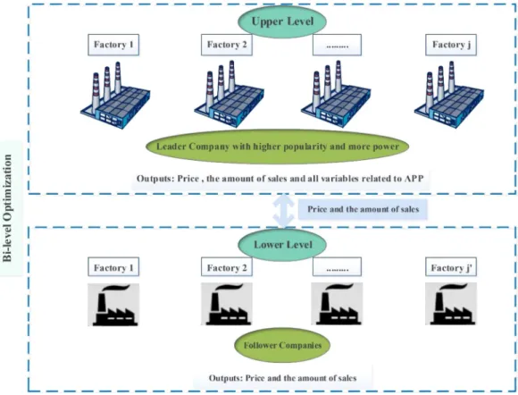
In the given problem, a leader company and sev-eral follower companies (rivals) are competing on the amount of sales and the selling price of products to acquire more revenue. The leader company, due to its background and higher popularity, has more power to acquire market share. The type of the competition in the market is pure, but the leader company is more known and older than its rivals. The main problem is that the leader company intends to produce some new products capable of replacing the existing products, while the rival companies do not intend and are not able to produce such new products. The amount of sales and the selling price of products for both the leader and the follower companies in addition to some variables related to the APP problem of the leader company should be appropriately determined. Because one manufacturer company has more power to acquire market share and act as a leader, the competition is modeled using BLP with regard to the concept of Stackelberg game [15], which properly matches the problem. Also, the basic APP model has been taken from the study by Makui et al. [7] and developed for the real competitive conditions. Figure 1 clearly illustrates the structure of the problem and the relationship between the leader and the follower in the competitive market.
This APP problem minimizes the costs to the leader company including production, setup, work-force, labor, inventory, hiring, and laying-o costs. Regarding the stochastic demand value, the model determines the production amount of product i in the manufacturing factory j by the workforce at level k in period t. Furthermore, the proposed model species the selling price, product inventory, number of the workforce, numbers of hiring and laying-o, and the amount of product that exceeds the demand for any type of product (over-fullment or oversupply). Since the revenue of the leader is deducted from the cost, the objective function of the leader is to minimize the total loss. The production problem for the rival companies has not been modeled due to special at-tention to production problem of the leader and the lack of information about rival companies. Therefore, the objective function of the follower will merely be maximization of the sales revenue.
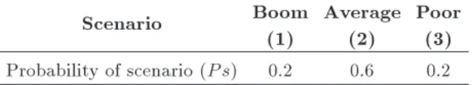
Considering the existing historical data and based on the comparison of the new products of the leader with similar products in the market, market demand along with some parameters of the APP is uncertain and they have inherently stochastic behavior in each period. This stochastic uncertainty can be a result of dierent factors such as change in the manner of customers and the existence of some complementary and alternative products. Thus, due to this uncertainty and because there is no information about their means and standard deviations to nd their distributions, regarding the historical data and opinions of the ex-perts, we only consider the states with the greatest probabilities instead of addressing all possible states of the uncertain parameters. It is clear that the states with the greatest probabilities are limited to some countable scenarios. Accordingly, some more probable scenarios with their probabilities of occurrence along with the value of each uncertain parameter in each scenario can be specied. The type of the considered uncertainty is a discrete stochastic variable of which the probability function is specied. Hence, scenario-based stochastic programming approach is the best approach to controlling and tackling this type of uncertainty. Finally, an extended version of this approach, known as the scenario-based robust stochastic programming,
introduced by Mulvey et al. [10] is used. Using
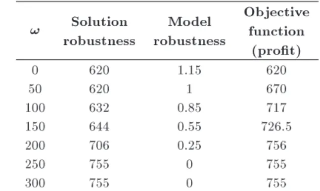
the scenario-based robust stochastic programming, the concepts of solution robustness and model robustness, which are illustrated in Section 5.3, can be integrated. It also should be noted that some basic studies have used this approach for the APP and they note that \as economic scenarios are taken into account, changes in uncertain data do not have signicant eect on an optimized production planning" [7,64]. The interested readers can refer to references [10,61,65-71] to obtain more information about the robust optimization
ap-proach. In this paper, the amounts of production and inventory are considered as control variables.
The main assumptions of the model are as follows:
The problem is multi-product and multi-period, and
the location of each factory is xed and predeter-mined;
Each manufacturing factory is able to produce
dif-ferent types of products in each period;
Production and inventory capacities of the leader
and selling capacity of the follower are assumed to be limited;
Fluctuating demand and some cost parameters are
naturally uncertain and controlled by a multi-scenario approach. The probability of each multi-scenario is estimated using the historical data and opinions of the experts;
The production of each product can be set up in
each period;
The leader company has more power to acquire
market share due to its higher popularity;
Although selling price is determined using the
pro-posed elasticity relations between demand and price, it should be in a specied range;
The elasticity relations between demand and price
are linearly determined using the historical data and regression relations.
In our model, the following main decisions are deter-mined under the competitive environment and uncer-tainty:
A) The main decisions of the leader include:
X The selling price and the amount of sales of the
nal product;
X The amount of production and inventory of
nal products;
X The number of workforce, including hired and
laid-o workforce.
B) The main decisions of the follower include:
X The selling price and the amount of sales of the
nal product.
Subsequently, rst, the elasticity relations be-tween demand and price are determined in general state. Then, the mathematical model is presented. 3.2. Presenting elasticity relations between
demand and price in general state
Assume that dL is the portion of the market demand
which the leader (L) potentially has and PL is the
price quoted by the leader. Also, assume that dF is
a portion of the market demand, which is potential for
follower. Regarding these quoted prices, the demand to the leader (L) and follower (F ) is determined by Eqs. (1) and (2); these demand-price equations are based on the economic theories in competitive markets in which a reverse relationship exists between price and demand [6]:
dL = L L:PL; (1)
dF = F F:PF: (2)
In these equations, Land F are respectively the price
elasticity of L (leader) and F (follower) to demand, indicating that with 1% increase in price, the demand
level is reduced by a few percent (L and F are both
positive).
Also, L and F indicate the selling power of L
and F in market, respectively:
PL= L dL
L ; (3)
PF = F dF
F : (4)
Obviously, assuming equality of Land F, if L> F,
then at the same demand level, the leader price can be higher according to Eq. (3). Parameter can be derived from factors such as quality, popularity, service level, and advertisement; thus, its higher values are desirable because there will be more power for sales.
Considering the reverse relationship between de-mand and prices, if both sellers produce the same product and are rivals, then the customer will consider their prices, simultaneously. Therefore, in the leader equation (Eq. (1)), the price of F and similarly, in the follower equation (Eq. (2)), the price of L will be eective. According to Eq. (1), if L increases its price, then the demand level for its products will be reduced. The same also holds for F based on Eq. (2). Now, it is obvious that if the market price of the rival (F ) is reduced, then the demand level of L will be reduced, and if the price of F is increased, then the demand level of L will be increased as well. Therefore, in a linear state, Eq. (5) can be proposed for developing Eq. (1) by considering the price of the rival (F ) [42]:
dL = L L:PL+ L:PF: (5)
Similarly, Eq. (6) is given for the follower (F ):
dF = F F:PF+ F:PL: (6)
In Eq. (5), L is dened as the price elasticity of
rival-demand for L, which implies that a unit of increase in
the price of F will increase the demand to L by %L.
3.3. Modeling using the bi-level programming In this section, using the BLP, a mathematical model is developed which considers the competition between the leader and the follower. The output of this model
will be the selling prices of the leader and the follower as well as the amount of sales of each one and the APP variables. The results obtained from the proposed model will be ecient for all the companies producing in the competitive market. In the following, the param-eters and decision-making variables will be introduced and then, the dened problem will be modeled. 3.4. Notations
Indices:
i Index of products
j Index of factories of leader company
j0 Index of factories of rival companies
k Index of workforce levels
s Index of uncertainty scenarios
t Index of time periods
Parameters:
ijt Leader's power to sell product i
produced by factory j at period t
0
ij0t Follower's power to sell product i
produced by factory j0 at period t
ijt Price elasticity of leader to demand
of product i produced by factory j at period t
0
ij0t Price elasticity of follower to demand
of product i produced by factory j0 at
period t
ijt Price elasticity of rival-demand from
leader for product i produced by factory j at period t
0
ij0t Price elasticity of rival-demand from
follower for product i produced by
factory j0 at period t
Ds
it Demand of product i at period t under
scenario s cps
ijkt The cost of producing each unit of nal
product i in factory j by workforce at level k during period t under scenario s cls
jkt Labor cost at level k in factory j
during period t under scenario s
cIfs
ijt Inventory cost of nal product i
in factory j during period t under scenario s
cwHjkt Cost of hiring workforce at level k in
factory j during period t
cwLjkt Cost of laying-o workforce at level k
in factory j during period t
aik The time needed to produce nal
product i by workforce at level k
bik The machinery time needed to produce
Ck Working hours of workforce at level k
in every period
LP Lijt Minimum selling price of nal product
i produced by factory j (leader) at period t
LP Fij0t Minimum selling price of nal product
i produced by factory j0 (rival) at
period t
UP Lijt Maximum selling price of nal product
i produced by factory j (leader) at period t
UP Fij0t Maximum selling price of nal product
i produced by factory j0 (rival) at
period t
CapLjt Maximum available inventory capacity
of all leader products in factory j at period t
CapFit Maximum selling capacity of product i
by follower companies in the market at period t
vfi Space occupied by a unit of product i
Mjt Maximum available machinery time in
factory j at period t
ckijt Cost of setting up the production of
nal product i in factory j at period t
Iwjk Number of initial workforce at level k
in factory j
ps Probability of scenario s
Fixed factor of deviation
! Penalty parameter
Large A large positive number
Decision variables: ps
ijkt Production amount of nal product
i in factory j by workforce at level k during period t under scenario s
prijt Selling price of nal product i produced
by factory j (leader) at period t pr0
ij0t Selling price of nal product i produced
by factory j0 (rival) at period t
Ifs
ijt Amount of inventory of nal product i
in factory j at period t under scenario s
xs
ijt Sales amount of nal product i
produced by factory j (leader) at period t
x0s
ij0t Sales amount of nal product i
produced by factory j0(rival) at period
t
dLs
ijt Amount of potential demand from
leader for nal product i produced by factory j at period t under scenario s
dFs
ij0t Amount of potential demand from
rival companies for nal product i
produced by factory j0 at period t
under scenario s
Wjkt Number of workforce at level k in
factory j at period t
wHjkt Number of workforce at level k hired
in factory j at period t
wLjkt Number of workforce at level k laid-o
in factory j at period t
kijt The binary variable of setting up nal
product i in factory j at period t
s
it The amount of higher response to
market demand (oversupply) for product i at period t under scenario s
s Deviation measure in scenario s
Now, the bi-level APP model is developed based on the real conditions of the competitive market of the leader and follower companies. The costs of the leader include Production Cost (PC), Setup Cost (SC), Workforce changing Cost (WC), Inventory Cost (IC), and Labor Cost (LC). Each of these costs, sales revenue for the leader company (RevL), and sales revenue for the follower companies (RevF) are obtained through the following equations:
Sales revenue for the leader company:
RevLs=
X
i
X
j
X
t
prijt:xsijt: (7)
Sales revenue for the follower companies:
RevFs=
X
i
X
j0
X
t
pr0
ij0t:x0sij0t: (8)
Production cost:
P Cs=
X
i
X
j
X
k
X
t
cps
ijkt:psijkt: (9)
Setup cost:
SCs=
X
i
X
j
X
t
ckijt:kijt: (10)
Workforce changing cost:
W Cs=
X
j
X
k
X
t
(cwHjkt:wHjkt
+ cwLjkt:wLjkt): (11)
Inventory cost:
ICs=
X
i
X
j
X
t
cIfs
ijt:Ifijts : (12)
LCs=
X
j
X
k
X
t
cls
jkt:Wjkt: (13)
Eq. (7) shows the sales revenue for the leader company, which is obtained by multiplying the selling price of its products by the amount of sales. Eq. (8) indicates the sales revenue for the rival companies. Eqs. (7) and (8) are nonlinear. Eqs. (9) and (10) show the total production cost and setup cost for the leader company, respectively. Eq. (11) shows the workforce changing cost including hiring and laying o. Eq. (12) shows the cost of inventory in warehouse and Eq. (13) shows the labor cost of dierent levels of workers for the leader company. In the following, objective functions of the leader and follower as well as the problem constraints will be separately presented. The leader's problem including its objective function and constraints is modeled as follows:
Leader:
min zL=
X
s
ps(P Cs+ SCs+ W Cs+ ICs
+ LCs RevLs) +
X
s
ps[(P Cs
+ SCs+ W Cs+ ICs+ LCs RevLs)
X
s0
ps0(P Cs0+ SCs0+ W Cs0
+ ICs0+ LCs0 RevLs0) + 2s]
+ !X
i
X
t
X
s
ps:its; (14)
s.t.:
Ifs
ijt= Ifij;t 1s +
X
k
(ps
ijkt) xsijt 8 i; j; t; s; (15)
X
j
dLs
ijt+
X
j0
dFs
ij0t its Dits 8 i; t; s; (16)
dLs
ijtijt ijt:prijt+ijt:pr0ij0t 8 i; j; j0; t; s;
(17) xs
ijt dLsijt 8 i; j; t; s; (18)
LP Lijt prijt UP Lijt 8 i; j; t; (19)
X
i
vfi:Ifijts CapLjt 8 j; t; s; (20)
Wjkt= Wjk;t 1+wHjkt wLjkt 8 j; k; t; (21)
X
i
aik:psijkt Ck:Wjkt 8 j; k; t; s; (22)
X
i
X
k
bik:psijkt Mjt 8 j; t; s; (23)
X
k
ps
ijkt Large:kijt 8 i; j; t; s; (24)
(P Cs+ SCs+ W Cs+ ICs+ LCs RevLs)
X
s0
ps0(P Cs0+ SCs0+ W Cs0+ ICs0
+ LCs0 RevLs0) + s 0 8 s; (25)
prijt;psijkt; Ifijts ; xsijt; dLsijt; Wjkt; wHjkt; wLjkt; its;
s 0; kijt 2 f0; 1g 8 i; j; k; t; s: (26)
In the upper-level objective function, i.e., Eq. (14), the company plays the role of a leader. This objective function, which should be minimized, is equal to the sum of the above-mentioned costs of the leader company minus its sales revenue. According to Mulvey et al.'s robust optimization approach [10], regarding various scenarios, the objective function of the leader in our BLP includes three terms. The rst and second terms are the mean and variance of the total loss, respectively, which measure solution robustness. The third term demonstrates model robustness regarding the infeasibility of the control constraints (16) under scenario s.
Eq. (15) is an equilibrium constraint used to determine the production amount of a product as well as the amount of inventory stored in the warehouse. Eq. (16) is a control equilibrium constraint, which determines the portions of the market demand that the leader and the follower can potentially have as well as the over-fulllment amount of customer demand (oversupply). In fact, this constraint implies that the total demand responded by the leader and the follower should not exceed the total market demand. If in period t, the total potential market demand for
the leader and follower, i.e., PjdLs
ijt + Pj0dFijs0t,
is higher than demand (Ds
it), then the total market
demand that becomes potential in reality in period t
will be equal toPjdLs
ijt+Pj0dFijs0t= Dits and sit=
P
jdLsijt +Pj0dFijs0t Dits indicates the oversupply.
It should be noted that s
i;t 1is not the oversupply for
period t, whereas, ifPjdLs
ijt+Pj0dFijs0tis less than
the demand, then the deviation will be equal to zero
(s
it = 0) after minimizing. Consequently, the total
market demand will not be satised.
Eq. (17) is the relation between demand and price, which has been written for the leader with regard to Eq. (5). Eq. (18) implies that the amount of sales of the leader for a particular product should not exceed its potential demand. Eq. (19) ensures that the
selling price of the leader is between the minimum and maximum.
According to Eq. (20), it is ensured that the inventory level of a certain company is less than its maximum available inventory capacity. Eq. (21) implies that the available workforce in each period is equal to the workforce in the previous period plus the change in the number of workforce in the current period. Considering the initial number of workforce
in factory j (Iwjk), this equation will be broken into
Eqs. (27) and (28):
Wjkt=Iwjk+wHjkt wLjkt 8 j; k; t=1; (27)
Wjkt=Wjk;t 1+wHjkt wLjkt 8 j; k; t 2: (28)
Eq. (22) restricts the production to the total hours available to the workforce at level k. Eq. (23) restricts the production in each period by workforce at level k to the available capacity of machinery production. Eq. (24) expresses the relationship between production of a product and production setup. Eq. (25) has been used in relation to robust optimization method to linearize the objective function of Mulvey et al.'s approach for the leader. Finally, Eq. (26) denes the decision variables of the leader.
In the following, the follower's problem including its objective function and constraints is modeled: Follower:
max zF =
X
s
ps:RevFs; (29)
s.t.
dFs
ij0t 0ij0t 0ij0t:prij0 0t+ ij0 0t:prijt
8 i; j; j0; t; s; (30)
x0s
ij0t dFijs0t 8 i; j0; t; s; (31)
X
j0
dFs
ij0t CapFit 8 i; t; s; (32)
LP Fij0t pr0ij0t UP Fij0t 8 i; j0; t; (33)
pr0
ij0t; x0sij0t; dFijs0t 0 8 i; j0; t; s: (34)
Eq. (29) presents the objective function of rival com-panies, which act in the BLP as the follower. Since the main goal in considering uncertainty in this research is to make the presented model more robust for the leader and the objective of the follower is of less importance, Eq. (29) is for maximization of the expected value of sales revenue of the rival companies.
Eq. (30) presents the relation between the demand and price for the follower with regard to Eq. (6). Eq. (31) indicates that the sales amount of the follower for a particular product should not exceed the demand
level that becomes potential for the follower. Eq. (32) expresses that the total potential demand for a certain product of the rival companies cannot exceed their sales capacity. Eq. (33) implies that the selling price of the follower should be between the minimum and
maximum. Finally, Eq. (34) denes the decision
variables of the follower. The constraints of the leader and the follower determine the feasible region for the leader.
3.5. Linearization of the objective functions First, it should be noted that BLP models are naturally nonlinear. However, we address the linearization of the bi-level function in the next section by transforming it into a uni-level one. As it is obvious, Eqs. (7) and (8) are nonlinear due to the multiplication of two continuous variables. Thus, they are linearized using a three-step approximate linearization method, which has been provided by researchers in the literature for linearizing such non-linear status [72]. First, Eq. (7) and then, Eq. (8) are linearized.
First step: For each of the continuous variables of Eq. (7), considering the constraints of the presented model, an upper and a lower bound are determined by Eqs. (35) and (36):
LP Lijt prijt UP Lijt 8 i; j; t; (35)
0 xs
ijt Dits 8 i; j; t; s: (36)
Second step: Multiplication of the two continuous variables of Eq. (7) is equal to, and replaced by, another continuous variable:
O1s
ijt = prijt:xsijt 8 i; j; t; s: (37)
Third step: Eqs. (38) and (39) are added to the constraints of the original model:
0 O1s
ijt Dits:prijt 8 i; j; t; s;
(38)
LP Lijt:xsijt O1sijt UP Lijt:xsijt 8 i; j; t; s:
(39) The same steps are also taken for Eq. (8):
First step: An upper and a lower bound are determined for each of the continuous variables of Eq. (8):
LP Fij0t pr0ij0t UP Fij0t 8 i; j0; t; (40)
0 x0s
ij0t CapFit 8 i; j; t; s: (41)
Second step: Multiplication of the two continuous variables is replaced by another continuous variable:
O2s
Third step: Eqs. (43) and (44) are added to the original model:
0 O2s
ij0t CapFit:prij0 0t 8 i; j0; t; s;
(43) LP Fij0t:x0sij0tO2sij0tUP Fij0t:x0sij0t 8 i; j0; t; s:
(44) 3.6. Transforming the bi-level problem into a
uni-level one using the KKT conditions To transform this bi-level programming problem into an ordinary uni-level problem, because all of the variables related to the follower are continuous, the KKT conditions can be used. Using such conditions, the objective function of the follower is replaced by constraints called constant and complementary condi-tions, which are added to the problem constraints with the objective function of the leader. In the following, objective function of the follower, in linear form, and its constraints are rewritten.
Follower:
max zF =
X
i
X
j0
X
t
X
s
ps:O2sij0t; (45)
s.t.:
dFs
ij0t 0ij0t ij0 0t:pr0ij0t+ ij0 0t:prijt
8 i; j; j0; t; s; (46)
x0s
ij0t dFijs0t 8 i; j0; t; s; (47)
X
j0
dFs
ij0t CapFit 8 i; t; s; (48)
pr0
ij0t UP Fij0t 8 i; j0; t; (49)
pr0
ij0t LP Fij0t 8 i; j0; t; (50)
O2s
ij0t CapFit:pr0ij0t 8 i; j0; t; s; (51)
O2s
ij0t LP Fij0t:x0sij0t 8 i; j0; t; s; (52)
O2s
ij0t UP Fij0t:x0sij0t 8 i; j0; t; s; (53)
x0s
ij0t; dFijs0t; prij0 0t; O2sij0t 0: (54)
Now, the KKT conditions should be written for the above model in order to transform the bi-level model into a uni-level one. For this purpose, rst, all the constraints of the problem, especially the constraints of non-negative variables, should be written as the standard state of a maximization problem. u1 and u10 are supposed to be variables related to the KKT conditions for the constraints of the above model. It should be noted that u9 and u10 are considered for
x0 0 and dF 0, respectively. It is not needed
to dene two variables related to the KKT conditions
for variables pr0 and O2 due to the application of
Constraints (50) and (52) and their intersection with
pr0 0 and O2 0, respectively. Now, the KKT
conditions can be written as follows:
ps= u6sij0t u7sij0t+ u8sij0t 8 i; j0; t; s; (55)
0 = 0
ij0t:u1sijj0t+ u4ij0t u5ij0t CapFit:u6sij0t
8 i; j; j0; t; s; (56)
0=u2s
ij0t+LP Fij0t:u7sij0t UP Fij0t:u8sij0t u9sij0t
8 i; j0; t; s; (57)
0=u1s
ijj0t u2sij0t+u3sit u10sij0t 8 i; j; j0; t; s; (58)
u1s
ijj0t M:(1 z1sijj0t) 8 i; j; j0; t; s; (59)
(dFs
ij0t ij0 0t+ij0 0t:prij0 0t ij0 0t:prijt)M:z1sijj0t
8 i; j; j0; t; s; (60)
u2s
ij0t M:(1 z2sij0t) 8 i; j0; t; s; (61)
(x0s
ij0t dFijs0t) M:z2sij0t 8 i; j0; t; s; (62)
u3s
it M:(1 z3sit) 8 i; t; s; (63)
(dFs
ij0t CapFit) M:z3sit 8 i; j0; t; s; (64)
u4ij0t M:(1 z4ij0t) 8 i; j0; t; (65)
(pr0
ij0t UP Fij0t) M:z4ij0t 8 i; j0; t; (66)
u5ij0t M:(1 z5ij0t) 8 i; j0; t; (67)
( pr0
ij0t+ LP Fij0t) M:z5ij0t 8 i; j0; t; (68)
u6s
ij0t M:(1 z6sij0t) 8 i; j0; t; s; (69)
(O2s
ij0t CapFit:prij0 0t)M:z6sij0t
8 i; j0; t; s; (70)
u7s
ij0t M:(1 z7sij0t) 8 i; j0; t; s; (71)
( O2s
ij0t+LP Fij0t:x0sij0t)M:z7sij0t
8 i; j0; t; s; (72)
u8s
ij0t M:(1 z8sij0t) 8 i; j0; t; s; (73)
(O2s
ij0t UP Fij0t:x0sij0t)M:z8sij0t
u9s
ij0t M:(1 z9sij0t) 8 i; j0; t; s; (75)
( x0s
ij0t) M:z9sij0t 8 i; j0; t; s; (76)
u10s
ij0t M:(1 z10sij0t) 8 i; j0; t; s; (77)
( dFs
ij0t) M:u10sij0t 8 i; j0; t; s; (78)
dFs
ij0t 0ij0t+ ij0 0t:pr0ij0t 0ij0t:prijt 0
8 i; j; j0; t; s; (79)
x0s
ij0t dFijs0t 0 8 i; j0; t; s; (80)
X
j0
(dFs
ij0t) CapFit 0 8 i; t; s; (81)
pr0
ij0t UP Fij0t 0 8 i; j0; t; (82)
pr0
ij0t+ LP Fij0t 0 8 i; j0; t; (83)
O2s
ij0t CapFit:prij0 0t 0 8 i; j0; t; s; (84)
O2s
ij0t+ LP Fij0t:x0sij0t 0 8 i; j0; t; s; (85)
O2s
ij0t UP Fij0t:x0sij0t 0 8 i; j0; t; s; (86)
x0s
ij0t 0 8 i; j0; t; s; (87)
dFs
ij0t 0 8 i; j0; t; s; (88)
u1s
ijj0t; u2sij0t; ; u10sij0t 0
8 i; j; j0; t; s; (89)
z1s
ijj0t; z2sij0t; ; z10sij0t2 f0; 1g
8 i; j; j0; t; s: (90)
Eqs. (55) to (58) are the equations related to the
gradient in the KKT method. Eqs. (59) to (78)
are the linear states of the complementary slackness conditions. Besides, Eqs. (59) and (60) are in fact the linear state of Eq. (91) and the remaining equations are linearized in the same way.
u1s
ijj0t: dFijs0t 0ij0t+ij0 0t:pr0ij0t ij0 0t:prijt
=0
8 i; j; j0; t; s: (91)
Eqs. (79)-(88) are the main constraints of the follower problem, which should be in the KKT conditions. Finally, Eqs. (89) and (90) dene the decision variables. Now, the developed model is a uni-level one in which objective function of the leader is the only objective of the problem and the constraints related to the KKT conditions have been replaced by the second level (follower).
4. Solution Approach
4.1. Introducing the Benders decomposition algorithm
According to a research by Makui et al. [7], the APP problems are among the strongly NP-hard problems and the use of meta-heuristic methods for solving such problems would not guarantee obtaining accurate and generally optimal solutions. Consequently, to overcome the computational complexities of the presented NP-hard problem, we need an ecient algorithm. Applying the BDA guarantees a global and accurate optimum solution. The BDA has a high ability in solving math-ematical problems in a large dimension, particularly in probabilistic cases. The BDA was rst presented by Benders [73] for solving linear optimization problems with complex variables. Nowadays, it is known as one of the most ecient algorithms for solving large-scale instances of Mixed-Integer Problems (MIPs). In BDA, instead of solving the original complex MIP, the problem is decomposed into a master problem (a pure integer programming) and a sub-problem (a linear programming). These two problems are repeatedly solved by applying the solution to one to another until the optimal solution is achieved. The BDA has considerable superiorities over other solution methods (such as meta-heuristic methods) including:
1. This algorithm is based on powerful algebraic
con-cepts;
2. Convergence of the algorithm and achievement of
optimal solution have been proved analytically;
3. Each decision-maker can set the optimality gaps
precisely.
These prots lead to the utilization of the BDA in var-ious contexts such as APP [7], planning of energy [74], SCND [75], and scheduling [76].
4.2. Implementing the BDA for the developed model
To develop the BDA for the current model, rst, the Dual Sub-Problem (DSP) and Master Problem (MP) should be formulated. To do this, rst, all the 0 and 1 variables, which complicate the problem, should be xed. These variables are listed below. Then, by replacing these xed variables in the primary model, the Primal Sub-Problem (PSP) is formulated. In order to avoid repetition, the PSP is not written.
Complex variable:
kijt, z1sijj0t, z2sij0t, z3its, z4ij0t, z5ij0t, z6sij0t,
z7s
ij0t, z8sij0t, z9sij0t, z10sij0t.
Fixed variable:
kijt, z1sijj0t, z2sij0t, z3its, z4ij0t, z5ij0t, z6sij0t,
If the dual variables corresponding to the PSP-constraints are written as w constraint number (e.g.,
the variable w15ijts is the considered dual variable
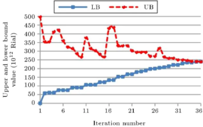
corresponding to Constraint (15) for i, j, t, and s), then the DSP, which produces an upper bound for the objective function of the original model in each repetition, will be formulated as follows:
Max : DSP =X
its
Ds
it:w16its+
X
ijj0ts
ijt:w17ijj0ts
+X
ijt
UP Lijt:w19aijt+
X
ijt
LP Lijt:w19bijt
+X
jts
CapLjt:w20jts+
X
jk;t1
Iwjk:w21jkt
+X
jts
Mjt:w23jts+
X
ijts
Large:kijt:w24ijts
+X
ij0ts
ps:w55ij0ts+
X
ijj0ts
M: 1 z1sijj0t
:w59ijj0ts
+ X
ijj0ts
M:z1sijj0t 0ij0t
:w60ijj0ts
+X
ij0ts
M: 1 z2sij0t
:w61ij0ts
+X
ij0ts
M:z2sij0t:w62ij0ts
+X
its
M: 1 z3sit:w63its
+X
ij0ts
M:z3sit CapFit:w64ij0ts
+X
ij0t
M: 1 z4ij0t:w65ij0t
+X
ij0t
M:z4ij0t UP Fij0t:w66ij0t
+X
ij0t
M: 1 z5ij0t:w67ij0t
+X
ij0t
M:z5ij0t+ LP Fij0t:w68ij0t
+X
ij0ts
M: 1 z6sij0t
:w69ij0ts
+X
ij0ts
M:z6sij0t:w70ij0ts
+X
ij0ts
M: 1 z7sij0t
:w71ij0ts
+X
ij0ts
M:z7sij0t:w72ij0ts
+X
ij0ts
M: 1 z8sij0t
:w73ij0ts
+X
ij0ts
M:z8sij0t:w74ij0ts
+X
ij0ts
M: 1 z9sij0t
:w75ij0ts
+X
ij0ts
M:z9sij0t:w76ij0ts
+X
ij0ts
M: 1 z10sij0t
:w77ij0ts
+X
ij0ts
M:z10sij0t:w78ij0ts
+ X
ijj0ts
0
ij0t:w79ijj0ts+
X
its
CapFit:w81its
+X
ij0t
UP Fij0t:w82ij0t+
X
ij0t
( LP Fij0t):w83ij0t;
(92) s.t.:
w25s+ ps:
X
s0
w25s0+ w38ijts+ w39aijts
+ w39bijts ps 8 i; j; t; s (93)
ijt:w17ijj0ts+ w19aijt+ w19bijt Dits:w38ijts
+ 0
ij0t:w60ijj0ts ij0 0t:w79ijj0ts 0
8 i; j; j0; t; s; (94)
ijt:w17ijj0ts ij0 0t:w60ijj0ts w66ij0t
+ w68ij0t+ CapFit:w70ij0ts
+ 0
ij0t:w79ijj0ts+ w82ij0t w83ij0t
CapFit:w84ij0ts 0
8 i; j; j0; t; s; (95)
+ cps
ijkt:w25s ps:cpsijkt
X
s0
w25s0
!
ps:cpsijkt 8 i; j; k; t; s; (96)
w15ijts w15ij;t+1;s+ vfi:w20jts+ cIfijts :w25s
ps:cIfijts
X
s0
w25s0
!
ps:cIfijts
8 i; j; t; s; (97)
w15ijts w18ijts 0 8 i; j; t; s; (98)
w62ij0ts LP Fij0t:w72ij0ts+ UP Fij0t:w74ij0ts
+ w76ij0ts+ w80ij0ts+ LP Fij0t:w85ij0ts
UP Fij0t:w86ij0ts w87ij0ts 0
8 i; j0; t; s; (99)
w16its !:ps 8 i; t; s; (100)
w25s 2:ps 8 s; (101)
w16its+ w17ijj0ts w18ijts 0
8 i; j; j0; t; s; (102)
w16its w60ijj0ts+ w62ij0ts+ w78ij0ts
+ w79ijj0ts w80ij0ts+w81its w88ij0ts0
8 i; j; j0; t; s; (103)
w21jkt cwHjkt 8 j; k; t; (104)
w21jkt cwLjkt 8 j; k; t; (105)
w21jkt w21jk;t+1 ck:w22jkts+ cljkts :w25s
ps:clsjkt
X
s0
w25s0
!
ps:clsjkt
8 j; k; t; s; (106)
w70ij0ts+ w72ij0ts w74ij0ts+ w84ij0ts
w85ij0ts+w86ij0ts 0 8 i; j0; t; s; (107)
0
ij0t:w56ijj0ts+ w58ijj0ts+ w59ijj0ts 0
8 i; j; j0; t; s; (108)
w57ij0ts w58ijj0ts+ w61ij0ts 0
8i; j; j0; t; s; (109)
w58ijj0ts+ w63its 0 8 i; j; j0; t; s; (110)
w56ijj0ts+ w65ij0t 0 8 i; j; j0; t; s; (111)
w56ijj0ts+ w67ij0t 0 8 i; j; j0; t; s; (112)
w55ij0ts CapFit:w56ijj0ts+ w69ij0ts 0
8 i; j; j0; t; s; (113)
w55ij0ts+ LP Fij0t:w57ij0ts+ w71ij0ts 0
8 i; j0; t; s; (114)
w55ij0ts UP Fij0t:w57ij0ts+ w73ij0ts 0
8 i; j0; t; s; (115)
w57ij0ts+ w75ij0ts 0 8 i; j0; t; s; (116)
w58ijj0ts+ w77ij0ts 0 8 i; j; j0; t; s; (117)
w15ijts;w21jkt; w55ij0ts; w56ijj0ts; w57ij0ts;
w58ijj0ts2 URS 8 i; j; j0; t; s; (118)
w16its;w17ijj0ts; w18ijts; w19aijt; w20jts;
w22jkts; w23jts; w24ijts; w38ijts;
w39aijts; w59ijj0ts; w60ijj0ts; w61ij0ts;
w62ij0ts; w63its; w64ij0ts; w65ij0t; w66ij0t;
w67ij0t; w68ij0t; w69ij0ts; w70ij0ts; w71ij0ts;
w72ij0ts; w73ij0ts; w74ij0ts; w75ij0ts; w76ij0ts;
w77ij0ts; w78ij0ts; w79ijj0ts; w80ij0ts; w81its;
w82ij0t; w83ij0t; w84ij0ts; w85ij0ts; w86ij0ts;
w87ij0ts; w88ij0ts 0 8 i; j; j0; t; s; (119)
w19bijt; w25s; w39bijts 0 8 i; j; t; s: (120)
Primal variables for the equations above are as follows:
Eq. (93): O1s
ijt, Eq. (94): pri;j;t
Eq. (95): pr0
ij0t, Eq. (96): psijkt
Eq. (97): Ifs
ijt, Eq. (98): xsijt
Eq. (99): x0s
ij0t, Eq. (100): its
Eq. (101): s, Eq. (102): dLsijt
Eq. (103): dFs
ij0t, Eq. (104): wHjkt
Eq. (105): wLjkt, Eq. (106): Wjkt
Eq. (107): O2s
ij0t, Eq. (108): u1sijj0t
Eq. (109): u2s
ij0t, Eq. (110): u3sit
Eq. (111): u4ij0t, Eq. (112): u5ij0t
Eq. (113): u6s
ij0t, Eq. (114): u7sij0t
Eq. (115): u8s
ij0t, Eq. (116): u9sij0t
Eq. (117): u10s
ij0t
Now, Based on the DSP solution, the MP is formulated as follows. In fact, the MP provides a lower bound on the objective function of the main model in each iteration.
Min MP = LB; (121)
s.t.:
LB X
s
ps:SCs+
X s ps " SCs X s0
ps0:SCs0
#
+X
its
Ds
it:w16its+
X
ijj0ts
ijt:w17ijj0ts
+X
ijt
UP Lijt:w19aijt+
X
ijt
LP Lijt:w19bijt
+X
jts
CapLjt:w20jts+
X
jk;t1
Iwjk:w21jkt
+X
jts
Mjt:w23jts+
X
ijts
Large:kijt:w24ijts
+X
ij0ts
ps:w55ij0ts+
X
ijj0ts
M: 1 z1s
ijj0t
:w59ijj0ts
+ X
ijj0ts
M:z1s
ijj0t 0ij0t
:w60ijj0ts
+X
ij0ts
M: 1 z2s
ij0t
:w61ij0ts
+X
ij0ts
M:z2s
ij0t:w62ij0ts
+X
its
M: (1 z3s
it) :w63its
+X
ij0ts
(M:z3s
it CapFit) :w64ij0ts
+X
ij0t
M: (1 z4ij0t) :w65ij0t
+X
ij0t
(M:z4ij0t UP Fij0t) :w66ij0t
+X
ij0t
M: (1 z5ij0t) :w67ij0t
+X
ij0t
(M:z5ij0t+ LP Fij0t) :w68ij0t
+X
ij0ts
M: 1 z6s
ij0t
:w69ij0ts
+X
ij0ts
M:z6s
ij0t:w70ij0ts
+X
ij0ts
M: 1 z7s
ij0t
:w71ij0ts
+X
ij0ts
M:z7s
ij0t:w72ij0ts
+X
ij0ts
M: 1 z8s
ij0t
:w73ij0ts
+X
ij0ts
M:z8s
ij0t:w74ij0ts
+X
ij0ts
M: 1 z9s
ij0t
:w75ij0ts
+X
ij0ts
M:z9s
ij0t:w76ij0ts
+X
ij0ts
M: 1 z10s
ij0t
:w77ij0ts
+X
ij0ts
M:z10s
ij0t:w78ij0ts+
X
ijj0ts
0
ij0t:w79ijj0ts
+X
its
CapFit:w81its+
X
ij0t
UP Fij0t:w82ij0t
+X
ij0t
( LP Fij0t) :w83ij0t; (122)
The right side of Eq. (123) 0; (123)
kijt; z1sijj0t; z2ijs0t; ; z10sij0t2 f0; 1g
8 i; j; j0; t; s: (124)
In the MP, the default values for the binary variables, which were considered equal to 1, are not used. In