Matrix Kummer-Pearson VII Relation and Polynomial Pearson VII Configuration Density

(1)

Vol. 11, No. 2, pp 217-230

Matrix Kummer-Pearson VII Relation and

Polynomial Pearson VII Configuration Density

Francisco J. Caro-Lopera1, Jos´e A. D´ıaz-Garc´ıa2

1_{Departmento de Ciencias B´}_{asicas, Universidad de Medell´ın, Colombia.} 2_{Departamento de Estad´ıstica y C´}_{alculo, Universidad Aut´}_{onoma Agraria} An-tonio Narro, M´exico.

Abstract. A case of the matrix Kummer relation of Herz (1955) based on the Pearson VII type matrix model is derived in this paper. As a con-sequence, the polynomial Pearson VII conﬁguration density is obtained and this sets the corresponding exact inference as a solvable aspect in shape theory. An application in postcode recognition, including a nu-merical comparison between the exact polynomial and the truncated conﬁguration density, is given at the end of the paper.

Keywords. Matrix Kummer relation, Pearson VII conﬁguration den-sity, zonal polynomials.

MSC: Primary: 62E15, 60E05, 43A90, 33C20; Secondary: 44A15.

1 Introduction

Start assuming that a given sample ofn“ﬁgures”, comprised inN

land-marks (“anatomical” points) in K dimensions, and summarized in an

N ×K matrix X, belongs to certain matrix variate distribution with

unknown scale and location parameters. The statistical theory of shape

pursues the distribution of the transforming X after ﬁltering out some

non important geometrical aspect of the original ﬁgures, such as the

Francisco J. Caro-Lopera([email protected]), Jos´e A. D´ıaz-Garc´ıa( ) (jadiaz@ uaaan.mx)

Received: February 1, 2012; Accepted: August 13, 2012

(2)

scale, the position, the rotation, the uniform shear, and so on; then the so called shape of the population object should be inferred and some comparisons among population shapes could be performed, among many others statistical comparisons in the shape space, instead of comparisons in the very noised non transformed Euclidean space. As usual, the clas-sical theory of shape, with different geometrical filters, as the Euclidean or affine, was based on Gaussian samples, see for example Goodall and Mardia (1993) and the references therein. Then, the non normal ap-plications demanded general assumptions for the samples, and the so termed generalized shape theory was set under elliptical models. Un-der the Euclidean filter we can mention the work of D´ıaz-Garc´ıa and Caro-Lopera (2010) and D´ıaz-Garc´ıa and Caro-Lopera (2012); they find the density of all geometrical information about the elliptical random

X which remains after removing the scale, the position and the

rota-tion. Finally, if an aﬃne ﬁlter is applied, in order to remove fromX all

geometrical information of scale, position, rotation and uniform shear,

Caro-Lopera et al(2010) obtained the so term conﬁguration density of

X. All the above densities are expanded in terms of the well known

zonal polynomials, in a series of papers by A.T. James in 60’s, see for example Muirhead(1982).

The transition of the Gaussian shape theory to the elliptical shape theory demanded some advances in integration involving zonal

polyno-mials (see for example Caro-Lopera et al(2010)), but important

prob-lems remain, the computability of the shape densities.

In this paper we focus in alternatives for such problems. It is easy to see in Goodall and Mardia (1993), D´ıaz-Garc´ıa and Caro-Lopera (2010) and D´ıaz-Garc´ıa and Caro-Lopera (2012) that the structure of shape densities under Euclidean transformations involves series of zonal poly-nomials which heritages the difficulties for computations of the classical hypergeometric series studied by Koev and Edelman (2006). However, a class of the generalized confluent type series of the configuration

densi-ties of Caro-Loperaet al(2010) can be handled in order to transformed

the series into polynomials, and then the addressed open problems for computations of the series can be avoided.

The conﬁguration density under Kotz type samples (including Gaus-sian) has this property, and the inference can be performed with

polyno-mials instead of inﬁnite series, see Caro-Loperaet al(2009). The source

for this property resides in a generalization of the Kummer relation of Herz (1955).

This motivates the present work, claiming that there is a similar

(3)

Kummer relation based on a Pearson VII distribution, which under cer-tain restriction of the parameters in the associated Pearson VII conﬁg-uration density, it can be turned into a polynomial density. Then the inference can be performed easily by working with the exact likelihood, which is written in terms of very low zonal polynomials. In fact the ex-act densities can be write down by using formulae for those polynomials; for example, in the planar shape theory (the most classical applications

resides in the study of ﬁgures in ℜ2), we can use directly the formulae

given by Caro-Lopera et al(2007) instead of the numerical approaches

by Koev and Edelman (2006), in order to perform some analytical prop-erties of the exact density.

This discussion is placed in the paper as follows: section 2 defines a Pearson VII type series and finds an integral representation that leads to a matrix Kummer type relation which we call Kummer-Pearson VII re-lation; then by applying some general properties studied by Herz (1955), the equality is extended for the required domains in the shape theory context. Finally, Kummer-Pearson VII relation gives the finiteness of the Pearson VII configuration density in section 3. Finally, section 4 studies an experiment of handwritten digit 3, and compares numerically the exact and the truncated associated estimates of the mean configu-rations.

2 Matrix Kummer-Pearson VII relation

Recall that the matrix Kummer relation (due to Herz (1955), see also Muirhead(1982)) states that

1F1(a;c;X) = etr(X)1F1(c−a;c;−X). (1)

Now, letX>0 be anm×mpositive deﬁnite matrix, then deﬁne

1P1(f(t,X) :a;c;X) =

∞ ∑

t=0

f(t,X) t!

∑ τ

(a)τ

(c)τ

Cτ(X), (2)

where the function f(t,X) is independent of τ, τ = (t1,· · · , tm), t1 ≥

t2· · · ≥tm>0, is a partition of t,

(β)τ =

m ∏ i=1

(

β−1

2(i−1)

) ti

, and

(b)t=b(b+ 1)· · ·(b+t−1), (b)0 = 1.

(4)

Then, using this notation we see that the Kummer relation (1) is a particular case of a general type of expressions with the following form

1P1(f(t,X) :a;c;X) =v(X)1P1(g(t,X) :c−a;c;h(X)), (3)

where the functionsv, gandhare uniquely determined by the particular

functionf and according to the domain of the parametersa,c and the

matrixX.

First, we consider an integral representation of the left hand side of

(3) under the model f(t,X) = (b)t.

Theorem 2.1. Let X < I, Re(a) >(m−1)/2, Re(c) > (m−1)/2

and Re(c−a) > (m−1)/2. Then for suitable reals b and d, we have that

1P1

(

(b)td−b−t:a;c;X

)

= Γm[c]

Γm[a]Γm[c−a]

×

∫

0<Y<Im

(d−tr(XY))−b|Y|a−(m+1)/2|I−Y|c−a−(m+1)/2(dY).(4)

Proof. First, we use a zonal polynomial expansion

(d−tr(XY))−b =

∞ ∑ t=0

(b)td−b−t

t! [tr(XY)]

t

=

∞ ∑ t=0

(b)td−b−t

t!

∑ τ

Cτ(XY).

Then integrating term by term using [Muirhead, 1982, theorem 7.2.10], we have that

∫

0<Y<Im

(d−tr(XY))−b|Y|a−(m+1)/2|I−Y|c−a−(m+1)/2(dY)

=

∞ ∑

t=0

(b)td−b−t

t!

∑ τ

∫

0<Y<Im

|Y|a−(m+1)/2 ×|I−Y|c−a−(m+1)/2Cτ(XY)(dY)

=

∞ ∑

t=0

(b)td−b−t

t!

∑ τ

(a)τ

(c)τ

Γm[a]Γm[c−a]

Γm[c]

Cτ(X)

= Γm[a]Γm[c−a]

Γm[c]

∞ ∑ t=0

(b)td−b−t

t!

∑ τ

(a)τ

(c)τ

Cτ(X)

= Γm[a]Γm[c−a]

Γm[c]

1P1

(

)

,

(5)

and the required result follows. Now, we derive the version of (1) but based on a Pearson VII type model, we call this expression, Kummer-Pearson VII relation.

Theorem 2.2. LetX>0,Re(a)>(m−1)/2,Re(c)>(m−1)/2and

Re(c−a) >(m−1)/2. Then for suitable reals b and d, the Kummer-Pearson VII relation is given by

1P1

(

)

= (d−trX)−b1P1

(

(b)t(d−trX)−t:c−a;c;−X

)

. (5)

Proof. Consider W=I−Y in (4), then we obtain

1P1

(

)

= Γm[c]

Γm[a]Γm[c−a]

×

∫

0<W<Im

(d−tr[X(I−W)])−b|W|c−a−(m+1)/2

×|I−W|a−(m+1)/2(dW)

= Γm[c]

Γm[a]Γm[c−a]

×

∫

0<W<Im

(d−trX−tr(−XW))−b|W|c−a−(m+1)/2

×|I−W|a−(m+1)/2(dW)

= Γm[c]

Γm[a]Γm[c−a]

× Γm[a]Γm[c−a]

Γm[c] 1

P1 (

(b)t(d−trX)−b−t:c−a;c;−X

)

,

which is the required result.

The reader can compare theorem 2.2 (and its proof) with the Kum-mer relation (and its proof given by Herz (1955)). So the analysis of Herz (1955) for extending the above relations for other values of the parameters, holds in the Kummer-Pearson VII relation too.

Explicitly, we proved that the integral representation (4) of1P1((b)t:

a;c;X) holds for Re(X)<I (by analytic continuation), Re(a)>(m−

1)/2,Re(c)>(m−1)/2 andRe(c−a)>(m−1)/2. Then by a suitable

modiﬁcation of the arguments in Herz (1955), we can extend the domain of (5) as follows.

(6)

Theorem 2.3. Re(X)>0,Re(a)>(m−1)/2andRe(c)>(m−1)/2. Then for suitable complex numbers b and d, the Kummer-Pearson VII relation is given by

1P1

(

)

= (d−trX)−b1P1

(

(b)t(d−trX)−t:c−a;c;−X

)

. (6)

The above relation is important in shape theory applications, in the

so called polynomial Pearson VII configuration density.

3 Polynomial Pearson VII Configuration

Density

Our motivation for studying ﬁnite shape densities, comes from the com-putations of hypergeometric series type involved in these distributions. It is known, that the zonal polynomials are computable very fast by Koev and Edelman (2006), but the problem now resides in the conver-gence and the truncation of the series of zonal polynomials. In fact, in the same reference of Koev and Edelman (2006) we read:

“Several problems remain open, among them automatic detection of convergence .... and it is unclear how to tell when convergence sets in. Another open problem is to determine the best way to truncate the series.”

Thus the implicit numerical difficulties for truncation of any config-uration density motivate two areas of investigation: first, continue the numerical approach started by (Koev and Edelman (2006)) with the confluent hypergeometric functions and extend it to the case of some configuration series type, as Pearson VII, Bessel, Logistic, for exam-ple; or second, propose a theoretical approach for solving the problem

analytically (see Caro-Loperaet al(2009)).

We study now the second question corresponding to the polynomial Pearson VII conﬁguration density.

Recall that ap×nrandom matrixXis said to have a matrix variate

symmetric Pearson type VII distribution with parameters s, R ∈ ℜ,

M :p×n,Σ:p×p,Φ :n×nwithR >0,s > np/2,Σ>0, and Φ>0 if its probability density function is

Γ[s]

(πR)np/2_{Γ [s}₋_np/2]_|_Σ_|n/2_|_Φ_|p/2 (

1+tr(X−M)

′_Σ−1₍_X₋_M₎_Φ−1

R

)−s

.

(7)

When s= (np+R)/2,Xis said to have a matrix variate t-distribution

withR degrees of freedom. And in this case, ifR= 1, thenXis said to

have a matrix variate Cauchy distribution, see Caro-Loperaet al(2010).

Then, by Caro-Lopera et al(2010) we have that (see Goodall and

Mardia (1993) for the gaussian case),

Lemma 3.1. Let be

A= ΓK[(N −1)/2]

πKq/2_|_Σ_|K/2_|_U′_Σ−1_U_|(N−1)/2_Γ

K[K/2]

, a= (N −1)/2, (7)

X=U′Σ−1µµ′Σ−1U(U′Σ−1U)−1/R, c=K/2, (8)

b=s−K(N −1)/2, d= 1 + tr(µ′Σ−1µ)/R. (9)

If Y ∼ EN−1×K(µN−1×K,ΣN−1×N−1 ⊗IK, h), for Σ > 0, then the

non-isotropic noncentral Pearson type VII configuration density is given by

A1P1 (

)

, (10)

where 1P1(·) has been defined in (2).

Unfortunately, the above conﬁguration density with general form

A1P1(f(t) : a;c;X) is an inﬁnite series, given that a= (N −1)/2 and

c=K/2 are positive (recall thatN is the number of landmarks,K is de

dimension andN−K−1≥1). So a truncation is needed for performing

inference when the modiﬁed algorithms of Koev and Edelman (2006) are used.

However the above series can be turned into a polynomial if we use

the following basic principle of Caro-Lopera et al(2009).

Lemma 3.2. Let beN−K−1≥1as usual, and consider the definition of 1P1(·) in (2). The infinite configuration density has the general form

CD1 =w(K, N,X) 1P1 (

f(t,X) : N −1

2 ;

K

2 ;X

)

,

for suitable functions: w(·), independent of t and τ but dependent of

K, N and X; andf(·), independent ofτ, but dependent oftand possibly of X (it depends on the generator elliptical function, compare with the particular Pearson VII case of lemma 3.1). Then, according to (3), if the dimension K is even (odd) and the number of landmarks N is odd (even), respectively, then the equivalent configuration density

CD2 =w(K, N,X)v(X) 1P1 (

g(t,X) :−

(

N −1

2 −

K 2

)

;K

2;h(X)

)

,

(8)

is a polynomial of degreeK((N−1)/2−K/2)in the latent roots of the matrixX(otherwise the series is infinite); wherev, gandhare functions understood in the context of (3) and depends on the elliptical generator function.

Given an elliptical conﬁguration densityCD1indexed by the function

f(·) and based in the fact that a= (N −1)/2 > 0, c = K/2 >0, the

crucial point here consists of ﬁnding an integral representation valid

for c −a = −(N −K −1)/2 < 0, which will lead to an equivalent

elliptical conﬁguration densityCD2indexed by some functiong(·). Then

the ﬁniteness of CD2 follows from K even (odd) and N odd (even),

respectively.

In particular, for the Pearson VII generator function, the referred polynomial density is provided by applying the new Kummer-Pearson VII relation of theorem 2.3, via lemma 3.2, in lemma 3.1.

Theorem 3.1. Let be A, a, b, c, dand X defined by (7)-(9).

If Y ∼ EN−1×K(µN−1×K,ΣN−1×N−1 ⊗IK, h), Σ > 0, K is even

(odd) andN is odd (even), respectively, then the polynomial non-isotropic noncentral Pearson type VII configuration density is given by

A(d−trX)−b1P1 (

(b)t(d−trX)−t:c−a;c;−X

)

, (11)

and it is a polynomial of degreeK((N−1)/2−K/2)in the latent roots of X.

Proof. The proof is trivial, just start with the inﬁnite conﬁguration density (10):

A1P1 (

)

,

where A, a, b, c, d and X are given by (7)-(9). Then apply (6) and the

result follows. Note that the ﬁniteness follows from Lemma (3.2) by

noting that c−a =−(N −K −1)/2 is a negative integer, when K is

even (odd) andN is odd (even).

The principle of lemma 3.2 is based on a known property of the

hy-pergeometric series easily extended to series of the type 1P1(f(t,X) :

a, c;X), see (2), which states that ifais a negative integer or a negative half integer, the series vanishes in a polynomial. Then if we have an application following a conﬂuent distribution type, it is a polynomial,

always that the parameteraaccepts the addressed special domain,

oth-erwise the distribution is a series of zonal polynomials and the open

(9)

problems for its computability remains. This last case occurs for exam-ple in the general configuration density, which is an infinite confluent

series type becausea= (N−1)/2>0, then it is not trivial to turn that

series into polynomials, because the application does not allow a nega-tive parameter. Then the lemma 3.2 gives a special subclass by selecting the number of landmarks (even, odd) given the dimension (odd, even), otherwise the conﬁguration density remains a series, then the associated Kummer relation must be obtained in order to transform the numerator

parameter aintoc−awhich is a negative half integer as required. So,

in the context of shape theory under aﬃne transformations, the study of Kummer relation type plays an important role. It is easy to check that the classical Kummer relation ﬁrst derive by Herz (1955), and set in the context of zonal polynomials by Constantine (1963) is related with a Gaussian kernel; but if we want to obtain some non Gaussian

polyno-mial densities (under the explained restrictions of N and K), then we

need to derive new Kummer relations; it was the case of certain class of Kotz conﬁguration densities (which includes the classical Gaussian), it required the derivation of the associated Kummer Kotz relation, see

Caro-Lopera et al(2009). Thus, in the case of the Pearson polynomial

conﬁguration density the corresponding Kummer relation was the key point for transforming series.

The above discussion opens related problems in some special topics of matrix variate analysis involving conﬂuent matrix with special domains for the parameters, or general hypergeometric series type with more or equal Pochhammer symbols in the numerator, several examples of this situations, which demands new developments for Euler relations and

similar ones, can be inferred from some distributions proposed in [?,

chapters 8–11].

4 An Application in Postcode Recognition

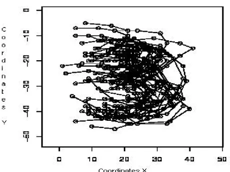
As an illustration of the impressive numerical advantage of the exact polynomial densities against the usual shape densities based con inﬁnite series of zonal polynomials, this section studies some aspects of a classi-cal example in statisticlassi-cal shape theory, the handwritten digit 3. Dryden and Mardia(1998) and other authors have studied the population mean shape of a collection of 30 handwritten number three. The codes were summarized in 13 landmarks, according the curvature of the extremes of the digit. Figure 1 (which was built with the R-package Shapes, au-thored by I. L. Dryden) shows the sample. The referred studies are based

(10)

on the assumption that the landmarks are randomly normal distributed and the shape of the object is reached under filtering out the scale, loca-tion and rotaloca-tion of the figure. However, the nature of the handwritten process seems to be far of a modeling with a similarity transformation and perhaps an affine transformation is closer to this situation, because the main uniform change of the construction of the figure appears pre-dominantly in one direction (vertical), simulating a spring type move-ment, instead of constant growing in all directions. In that case we remove all geometrical information of the figure which is related with the scale, location, rotation and uniform shear. An statistical proof of this statement can be obtained by using dimension model theory, based

on modiﬁcations of the so calledBIC∗ criterion, see Raftery(1995),

Ris-sanen(1978), Yang and Yang(2007), and the references there in. The corresponding statistical proof for this experiment under a Gaussian generator and aﬃne transformation against an Euclidean law is given

by Caro-Loperaet al(2009).

Table 1: The maximum likelihood estimates of conﬁguration location

Truncation Convergence Time Loglikelihood Iterations FuncCount Seg.

Series 0 N 195 2.2093e+003 15974 20000

Polynomial 0 Y 120.8906 2.1219e+003 8367 10479

Series 5 N 284.5781 2.1686e+003 15977 20000

Polynomial 5 Y 147.4219 1.5346e+003 7854 9914

Series 10 N 361.1563 1.8315e+003 15927 20000

Polynomial 10 Y 228.7500 1.3223e+003 10111 12633

Series 20 Y 378.4844 1.6994e+003 12853 16115

Polynomial 20 Y 299.3594 1.3223e+003 10111 12633

Series 50 Y 532.2656 1.5287e+003 9622 12037

Polynomial 50 Y 521.9375 1.3223e+003 10111 12633

Series 100 Y 1.1054e+003 1.4244e+003 10971 13731

Polynomial 100 Y 883.4219 1.3223e+003 10111 12633

Series 120 Y 957.0781 1.4023e+003 7768 9704

Polynomial 120 Y 901,5687 1.3223e+003 10111 12633

Series 150 Y 1.5775e+003 1.3787e+003 10068 126515

Polynomial 150 Y 1.2637e+003 1.3223e+003 10111 12633

Template

Tables 1, 2 and 3 shows the conﬁguration location estimates by us-ing two methods, the classical one (based on an inﬁnite series of zonal polynomials, see lemma 3.1) and the polynomial density obtained by the matrix Kummer-Pearson relation (see theorem 3.1); the truncation of the series, the time in seconds and the convergence of the algorithms are given in the corresponding columns; also it is shown the number of iterations and functions being evaluated in the optimization routine and the maximum value reached in the likelihood. Finally, the tables

(11)

Table 2: ...Continuation Table 1

V1 V2 V3 V4 V5

Series

[

−0.9965 0.3517

] [

0.0709

−0.2434

] [

0.0695

−0.3486

] [

0.4455

−0.5559

] [

0.2338 0.4746

]

Polynomial

[

0.0558 0.6188

] [

−0.2476 0.3414

] [

−0.455

−0.0065

] [

−0.5717

−0.3417

] [

−0.435 0.0312

]

Series

[

−0.4139 2.1333

] [

0.2583 1.1821

] [

−1.2376 1.9376

] [

−0.7693

−0.3752

] [

−1.0877 0.0451

]

Polynomial

[

−1.4363 1.7525

] [

−3.0789 1.5125

] [

−3.7258 0.884

] [

−3.7155 0.109

] [

−3.521 0.763

]

Series

[

0.0556 1.0517

] [

−0.3136 0.7415

] [

−0.5988 0.2595

] [

−0.7255

−0.2247

] [

−0.5666 0.2315

]

Polynomial

[

−1.2968 2.6833

] [

−3.1351 2.2759

] [

−3.9553 1.291

] [

−4.0714 0.0888

] [

−3.7561 1.1051

]

Series

[

0.0668 1.3995

] [

−0.4858 1.0199

] [

−0.8513 0.3873

] [

−1.049

−0.2859

] [

−0.8157 0.324

]

Polynomial

[

−1.2968 2.6833

] [

−3.1351 2.2759

] [

−3.9553 1.291

] [

−4.0714 0.0888

] [

−3.7561 1.1051

]

Series

[

−0.0738 1.8964

] [

−0.9106 1.4216

] [

−1.4161 0.5915

] [

−1.6445

−0.3127

] [

−1.345 0.4978

]

Polynomial

[

−1.2968 2.6833

] [

−3.1351 2.2759

] [

−3.9553 1.291

] [

−4.0714 0.0888

] [

−3.7561 1.1051

]

Series

[

−0.3405 2.216

] [

−1.456 1.7225

] [

−2.0655 0.7939

] [

−2.2739

−0.2482

] [

−1.9498 0.6722

]

Polynomial

[

−1.2968 2.6833

] [

−3.1351 2.2759

] [

−3.9553 1.291

] [

−4.0714 0.0888

] [

−3.7561 1.1051

]

Series

[

−0.4354 2.2876

] [

−1.6332 1.7975

] [

−2.2695 0.8526

] [

−2.4668

−0.2183

] [

−2.1407 0.7234

]

Polynomial

[

−1.2968 2.6833

] [

−3.1351 2.2759

] [

−3.9553 1.291

] [

−4.0714 0.0888

] [

−3.7561 1.1051

]

Series

[

−0.5634 2.3686

] [

−1.8664 1.8863

] [

−2.5352 0.9255

] [

−2.7168

−0.1767

] [

−2.3905 0.7869

]

Polynomial

[

−1.2968 2.6833

] [

−3.1351 2.2759

] [

−3.9553 1.291

] [

−4.0714 0.0888

] [

−3.7561 1.1051

]

Template

[

−2.0908 2.2071

] [

−4.0409 2.8051

] [

−4.5904 2.2904

] [

−4.2069 1.3688

] [

−3.3126 1.7582

]

show the maximum likelihood estimates of conﬁguration location. It is important to note that the exact conﬁguration density is just a polyno-mial of 10 degree, which can be constructed by using the exact formulae

given by Caro-Lopera et al(2007). Also, observe that all the estimates

after this truncation are equal, as it can be noticed in the table. How-ever, the estimates based on the truncation of the series given in lemma 3.1) are so unstable, in fact, it is not sufficient a truncation of 120 in the modification of the algorithms of Koev and Edelman (2006) to ob-tain the exact estimation. Moreover, the computations were performed with a processor Intel(R) Corel(TM)2 Duo CPU, [email protected], and 2,96GB of RAM, and we tried to obtained an estimation with a trun-cation of 150, with the same initial values, and the programm does not tolerate that truncation. Tables also shows the configuration

(12)

Table 3: ...Continuation Table 1

V6 V7 V8 V9 V10

Series

[

−0.2582 0.4178

] [

0.0624

−0.3006

] [

0.117 0.0974

] [

−0.1171 0.0412

] [

−0.1083 0.5711

]

Polynomial

[

−0.393 0.1695

] [

−0.4416 0.2615

] [

−0.6074 0.0661

] [

−0.7698

−0.3256

] [

−0.822

−0.6514

]

Series

[

−0.251 2.519

] [

−0.5782 1.5909

] [

−1.0868

−0.1355

] [

−1.0048

−0.8559

] [

−1.4068 0.3555

]

Polynomial

[

−3.7978 1.2843

] [

−4.5051 1.6567

] [

−5.2428 1.3901

] [

−5.3697 0.5387

] [

−4.8461

−0.3302

]

Series

[

−0.5192 0.5463

] [

−0.5901 0.7407

] [

−0.794 0.4857

] [

−1.0118

−0.1144

] [

−1.0649

−0.668

]

Polynomial

[

−3.983 1.9115

] [

−4.708 2.4794

] [

−5.5607 2.0488

] [

−5.8348 0.7249

] [

−5.395

−0.6145

]

Series

[

−0.7521 0.7489

] [

−0.8495 0.9931

] [

−1.1504 0.6829

] [

−1.4295

−0.101

] [

−1.5055

−0.8253

]

Polynomial

[

−3.983 1.9115

] [

−4.708 2.4794

] [

−5.5607 2.0488

] [

−5.8348 0.7249

] [

−5.3955

−0.6145

]

Series

[

−1.2986 1.0772

] [

−1.493 1.4286

] [

−1.9345 1.0284

] [

−2.2848

−0.0132

] [

−2.318

−0.9888

]

Polynomial

[

−3.983 1.9115

] [

−4.708 2.4794

] [

−5.5607 2.0488

] [

−5.8348 0.7249

] [

−5.3955

−0.6145

]

Series

[

−1.9591 1.3502

] [

−2.2843 1.784

] [

−2.8528 1.3471

] [

−3.2177 0.1607

] [

−3.1477

−0.9718

]

Polynomial

[

−3.983 1.9115

] [

−4.708 2.4794

] [

−5.5607 2.0488

] [

−5.8348 0.7249

] [

−5.3955

−0.6145

]

Series

[

−2.1715 1.4227

] [

−2.5401 1.8768

] [

−3.1444 1.4358

] [

−3.5064 0.2207

] [

−3.3982

−0.946

]

Polynomial

[

−3.983 1.9115

] [

−4.708 2.4794

] [

−5.5607 2.0488

] [

−5.8348 0.7249

] [

−5.3955

−0.6145

]

Series

[

−2.4511 1.5105

] [

−2.8769 1.9884

] [

−3.5264 1.5443

] [

−3.8811 0.2992

] [

−3.7205

−0.9059

]

Polynomial

[

−3.983 1.9115

] [

−4.708 2.4794

] [

−5.5607 2.0488

] [

−5.8348 0.7249

] [

−5.3955

−0.6145

]

Template

[

−3.5881 2.7053

] [

−5.4996 4.0629

] [

−7.5557 4.8428

] [

−8.2514 4.4208

] [

−6.9108 2.8899

]

nates of the template digit 3, a ﬁgure consisting of two equal sized arcs, and 13 landmarks (two coincident) lying on two regular octagons see Dryden and Mardia(1998), p.153. Finally a test about the equality of the conﬁguration shape and the templates indicates an approximate zero p-value, the same conclusion obtained by Dryden and Mardia(1998) and

Caro-Loperaet al(2009) by using other approaches.

Acknowledgment

The authors wish to thank the Editor and the anonymous reviewers for their constructive comments on the preliminary version of this paper. The ﬁrst author was supported by Universidad de Medell´ın-Colombia grant No. 158.

(13)

Figure 1: Sample of 30 handwritten digit 3.

References

Caro-Lopera, F. J., D´ıaz-Garc´ıa, J. A., and Gonz´alez-Far´ıas, G. (2007),

A formula for Jack polynomials of the second order. Applicationes

Mathematicae,34, 113–119.

Inference in statistical shape theory: elliptical conﬁguration

den-sities. Journal of Statistical Research,43(1), 1–19.

Noncentral Elliptical Conﬁguration Density. Journal of

Multivari-ate Analysis,101(1), 32–43.

Constantine, A. G. (1963), Noncentral distribution problems in

multi-variate analysis. The Annals of Mathematical Statistics,34, 1270–

1285.

(14)

D´ıaz-Garc´ıa, J. A. and Caro-Lopera, F. J. (2012), Generalised shape

theory via SVD decomposition I. Metrika, 75, 541-565.

D´ıaz-Garc´ıa, J. A. and Caro-Lopera, F. J. (2012), Statistical theory of shape under elliptical models and singular value decompositions.

Journal of Multivariate Analysis, 103, 77-92.

Dryden, I. L. and Mardia, K. V. (1998), Statistical Shape Analysis. Chichester: John Wiley & Sons Inc.

Goodall, C. R. and Mardia, K. V. (1993), Multivariate aspects of shape

theory. The Annals of Statistics,21, 848–866.

Herz, C. S. (1955), Bessel functions of matrix argument. The Annals

of Mathematics,61, 474–523.

Koev, P and Edelman, A. (2006), The eﬃcient evaluation of the hyper-geometric function of a matrix argument. Mathematics of

Com-putation, 75, 833-846.

Muirhead, R. J. (1982), Aspects of Multivariate Statistical Theory. Wi-ley Series in Probability and Mathematical Statistics, John WiWi-ley & Sons, Inc.

Raftery, A. E. (1995), Bayesian model selection in social research.

So-ciological Methodology, 25, 111–163.

Rissanen, J. (1978), Modelling by shortest data description.

Automat-ica,14, 465–471.

Yang, Ch. Ch. and Yang, Ch. Ch. (2007), Separating latent classes

by information criteria. J. Classiﬁcation,24, 183–203.