HIERARCHICAL MODELLING OF INDOOR AND OUTDOOR (RESIDENTIAL) RADON DATA (RRD)

HIERARCHICAL MODELLING OF INDOOR AND

OUTDOOR (RESIDENTIAL) RADON DATA (RRD)

G.A*1_{. DAWODU AND A.O. MUSTAPHA}2

1_{Department of Statistics, College of Natural Sciences, Federal University of Agriculture,}

Abeokuta (FUNAAB), Abeokuta, Nigeria.

2 _{Department of Physics, College of Natural Sciences, Federal University of Agriculture,}

Abeokuta (FUNAAB), Abeokuta, Nigeria.

*Corresponding author: : abayomidawodu@yahoo.co.uk Tel: +2348033753735

cannot be emphasized because the inhabi-tants of such a community will always desire to know how “friendly” their environment is with respect to “freely available”, carcino-genic radioactive radon, more so, if they share their neighbourhoods with rocks, and quarries, Electricity and nuclear power sta-tions (the Chernobyl and Fukushima are two notable accidents that victims cannot forget easily). Even when there are no accidents,

ABSTRACT

This work, proposes a Hierarchical Modelling (HM) for the indoor and outdoor Residential Radon Data (RRD). Indoor RRD and outdoor RRD are seen as distinct “hierarchies” of carcinogenic radioactive radon and both hierarchies constitute the least exposure that can be experienced by an individual. Works on this issue have always been based on complicated models, even for single instances of both indoor and outdoor residential radon. Our proposed method can be used to analyse effectively the many-to-many (it, however, becomes numerically clumsy if more than 5-to-5 instances are considered) instances of residential radon, although we have illustrated, here, using a three-to-three situation. Our preference of this method is based on its simplicity, and probable higher precision, as compared with the complexity involved in other methods on the same issue. The data used for the illustration of our models were taken from the indoors (i.e. living-room, bedroom and the kitchen) and the rest outdoors (i.e. verandah, car-park and the well-water shed) of a residential building in a lightly populated estate (i.e. Asero housing estate). Observations were taken on a daily basis throughout the dry season cov-ering ninety days (i.e. January, February and March), this constitutes our season I (i.e. dry). The same was repeated in the season II (i.e. wet) which was taken at the beginning of June through July and August.

Key words: HM, RRD, Ordinary Least Squares (OLS), Pseudo-clusters and Pseudo-strata,

R packages.

INTRODUCTION

Enough has been said about potential risks and health hazards associated with elevated levels of residential radon (Al Zabadil et al, 2012; Chege et al, 2009; Darby et al, 2001; Fitzpatrick-Lewis et al, 2010; Nero et al, 1994; Price, 1995; Singh, 2010; Smith and Oleson, 2008). The need to assess the least and maximum exposures, a hypothetical member of a community can experience,

Science, Engineering and Technology Print - 2277 - 0593

Online - 2315 - 7461

inhabitants of “rocky” environments such as those obtainable in Abeokuta, Ogun state, Nigeria have enough to worry about concerning carcinogenic radon. Concerning HM, there are locations; within a household (e.g. sitting (living) room, kitchen, toilets and bedroom) termed as indoor areas, be-tween households (e.g. children play areas and immediate environments or com-pounds, verandas and car parking areas) termed as outdoor areas. These two catego-ries of areas are identified as “hierarchies” or levels and to each of them pertinent models are fitted; In the aggregate of the two hierarchies are models upon which the statistical analyses are based. The fact that factors involved with RRD (i.e. Tempera-ture, Pressure, Relative-Humidity etc.) are all quantifiable makes it seem natural for us to expect the radon emission to be a func-tion of the levels of these variables also. Hence, either way, we can say that “there are hierarchies among the physical compo-nents of residential radon as well as the lo-cality within which it is found”.

DATA COLLECTION

by SARAD GmBh, Germany) consist of six distinct units three of which were placed indoors (i.e. living-room, bedroom and the kitchen) and the rest outdoors (i.e. veran-dah, car-park and the well-water shed). Ob-servations were taken on a daily basis throughout the dry season covering ninety days (i.e. January, February and March), this constitutes our season I (i.e. dry). The same was repeated in the season II (i.e. wet) which was taken at the beginning of June through July and August. Radon Scout measures radon concentration in Bq m-3_{, as}

well as Temperature in o_{C, Relative}

humid-ity in percentage of concentration etc. But

this present work is based on the measured radon concentration alone.

METHODOLOGY

A methodology of HM, entails that we write two models (Wright and London, 2009), each of which will capture the scenario at each of the two identified hierarchies within a hypothetical residence (i.e. indoor and out-door). Now, let us first assume, for the sake of brevity that there is one instance each of both hierarchies (i.e. indoor and outdoor). That is predictor y for indoor and v for out-door.

Let us first consider regression models in which only intercepts vary (i.e. equal slopes), use the index, j, for a hypothetical indoor radon measurement and k, for the outdoor radon measurement associated with the in-door j. Then, we have;

Where and are estimators, and

are independent residual quantities, at the indoor and outdoor radon hierarchies respectively.

However both the intercept and slope can be allowed to vary but the work will become cumbersome (Gelman and Hill, 2007); the pertinent model for this situation is as stated below (equation 3.2):









, 1, 2,...,

, 1, 2,..., (3.1)

j k j j

k k k

x y j m indoor

a bv k K outdoor

  

 

   

   

j

y v_k j

k



 













1 1 2

, 1,2,...,

, 1,2,..., (3.2)

, 1,2,...,

j k j j j

k k k

k k k

x y j m indoor

a bv k K outdoor

a bv k K outdoor

                  

However, use HM whenever your data is grouped (or nested) in more than one cate-gory (for example, states, countries, etc). HM will allow its user to; study the effects that vary entity by entity (or group-by-group), and estimate group level averages, now, this is a vital advantage because regu-lar regression ignores the average variation between entities. Besides, individual regres-sion may face sample problems and lack of generalization.

Further discussion on these two models, concerning radon, can be found in Gelman (2005), Gelman (2006), Gelman and Hill (2007) and Tranmer and Elliot (2007). Pioneering works of HM can be found in Goldstein (1986), Goldstein and McDonald (1988) and Goldstein (1991). A series of approaches can be found in works such as; Bates (2005), Hedeker (2007), Bolker et al (2008), Skrondal and Rabe-Hesbeth (2009), Wright and London (2009), Kenny and Hoyt (2009), Nikita (2010), Grilli and Ram-pichini (2012), and Schliep and Hoeting (2013).

Our proposed method assumes that each multilevel is actually a “poly-level” that can be split into two or more levels (according to similarity, convenience and the number of instances involved altogether) or com-partments in such a way that data entries in the same level are as similar as possible (with respect to the characteristics under study). It sustains but pays little attention to spacial proximity as a way of trading it off for higher “precision”. To make things clearer, our work purports to carry-out analysis on the statistical states of the radon emission concentration of just adequately populated residential buildings in a social elites area (i.e. Asero housing estate) of Ogun state to enable our audience to infer

from it the quantity of radon concentration the inhabitants of Ogun state, in general are exposed to on a daily basis. Towards this end we start by saying let us see the entire analy-sis as a multilevel involving two levels (i.e. indoor and outdoor) which will bring to rele-vance either of the two models (i.e. (3.1) or (3.2) above), but rather since the demarca-tion into “indoor” and “outdoor” is not “too” vital to our analysis (or, at least, not as important as having a high precision measure of the said radon emission concentration), we “trade” it off for higher precision and see the problem as a HM with six hierarchies (each representing one of the six locations where our radon scout equipment were kept). Albeit our data entry procedure will not be devoid of the original classification into two (indoor and outdoor) areas but what is more important is the fact that the data entries within a hierarchy (i.e. indoor or outdoor) are as similar as possible. Hence the two hierarchies are seen as clusters” within each of which are “pseudo-strata” (the three distinct locations).

Our statistical analysis recognizes the fact that, and indeed assumes that, observations from distinct pseudo-strata in the same pseudo-cluster may be correlated. In the mathematical analysis used to examine the effects of this correlation, we let i refer to the day (i.e. replication), j to the pseudo-cluster and k to the pseudo-stratum; such that, for strata in the same pseudo-cluster, subscripts i and j will be the same per day. We assume that there exists a

correlation between the experimental errors and for any pair of distinct pseudo-strata in the same pseudo-cluster. However, strata in distinct pseudo-clusters may be uncorrelated. Thus, we have



iju

It is also possible that we have, in each pseudo-stratum two or more entries. Al-though there are two seasons involved with our RRD (i.e. wet and dry), but we may have reasons to take radon readings during the day and night. However, with two read-ings per pseudo-stratum, the error variance of a pseudo-cluster total becomes;

(3.4) The factor 2 is regarded as representing the effects of adding over two readings in each pseudo-stratum. Hence the error variance

per pseudo-stratum is With m

pseudo-strata per pseudo-cluster, the

corre-sponding error variance is .

On the other hand, the error variance from the difference in the two readings in a pseudo-stratum gives;

(3.5)









   





2

,

3.3 0,

iju stv

if i s j t E

if i s j t 

 

   

  

  

 





1 .

 









2

1 m 1

   









1 2 2 1

st st

E     

Equation (3.5) is also the effective variance per pseudo-stratum and is invariant, irrespec-tive of the number of readings inside a pseudo-stratum. With our RRD, (i.e. correlation coefficient is always positive). As explained earlier in this work, the main ef-fects of the pseudo-clusters (which will be referred to as A, for brevity) are less pre-cisely estimated, as a trade-off for that of the pseudo-strata (which will be B, for brevity) and consequently, of the AB interaction. As for the analysis of variance, we first com-pute the six pseudo-strata totals. Their sum of squares of deviations is partitioned in the usual way into 1 d.f. (i.e. degree of freedom) for replication, 1 for the main effects of A, and 1 for the experimental error applicable to a whole pseudo-cluster. All computations are divided by 2 to convert them to a pseudo -stratum basis. The six differences provide 2 d.f. which represents the main effect of B, 2 d.f. which represent the AB interactions, and the remaining 4 d.f. whose mean square gives an unbiased estimate of the

pseudo-strata error variance . All sums

of squares are again divided by 2. The com-plete separation of degrees of freedom is shown in the table 1 below:

0  





2

1

 





 

 





 

st st st st st st

E  E E E      

Table 1: Analysis of variance for experiments where pseudo-strata are within pseudo-clusters.

Degree of freedom (d.f.) Whole pseudo-clusters

Replications 1

A 1

Pseudo-cluster error 1

Total 3

Pseudo-strata B 2

AB 2

Pseudo-strata error 4

If the pseudo-clusters are in locations and the pseudo-strata are in locations, the subdivision of degrees of freedom in





the analysis of variance is shown in table 2 below where pseudo-clusters are arranged in randomized blocks (r replicates):

Table 2: Partition of degrees of freedom for pseudo-strata within pseudo-cluster experiment.

Sources d.f. Blocks (r – 1) Pseudo-clusters (A)

Error (A) Total

Pseudo-strata (B) AB Error (B)

Total































  





r

 

Let and be the error mean squares for error (A) and error (B) respectively, on a pseudo-stratum basis. For the means, also

A

 B expressed on a pseudo-stratum basis, the

standard errors shown in the table 3 below are pertinent:

The last comparison in table 3 contains both the main effect of pseudo-cluster and the (pseudo-cluster)(pseudo-stratum) inter-action; consequently the appropriate error is a weighted mean of and . This er-ror also applies to the difference between two pseudo-clusters means which have dif-ferent levels of pseudo-strata.

Now, let tA , tB be the significant levels of

“t” corresponding to the degrees of free-dom in and , respectively. The sig-nificance level of “t” is;

(3.6).

RESULTS

Table 4 contains an extract from our RRD,

with indoor observations denoting indoor RRD (with its three locations observations

A

 B

A

 _B









1 1

B B A A

B A

t t

t   

  

 



 

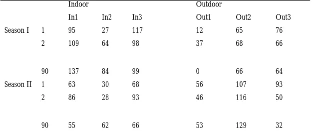
(i.e. In1, In2 and In3), and outdoor observa-tions denoting outdoor RRD (with its three locations observations (i.e. Out1, Out2 and Out3). The observations spans through ap-proximately three months (duration per sea-son) and entries are recorded on a daily ba-sis, the unit of measurements is “Bq/m3_”.

Without loss of generality, we assume that our RRD can still be treated as randomized blocks scheme with 90 replications.

It is customary to compute the analysis of variance on a pseudo-strata basis. For avoid-ance of confusion, this will be stated clearly in the analysis of variance table itself.

The calculations involved can be presented in the following three steps.

Step I: Obtain the pseudo-cluster totals by the method appropriate to the design in which they are arranged.

Table 3: Standard errors for the pseudo-strata in pseudo-cluster experiment.

Comparisons Standard Errors

Difference between two pseudo-clusters means:

Difference between two pseudo-strata means:

Difference between two pseudo-strata means at the same level of pseudo-cluster: Difference between two pseudo-cluster means at the same level of pseudo-strata or

At different levels of pseudo-strata:

0 . 5

2 A

r

 

 

 

 

0 . 5

2 _B

r

 

 

 

 

0 . 5

2 B

r



 

 

 

 

  0 . 5

2 1 B A

r

  



   

 

 

Table 4: An extract of our RRD showing the way it was constructed from the in doors and outdoors observations.

Indoor Outdoor

In1 In2 In3 Out1 Out2 Out3

Season I 1 95 27 117 12 65 76

2 109 64 98 37 68 66

_

90 137 84 99 0 66 64

Season II 1 63 30 68 56 107 93

2 86 28 93 46 116 50

_

90 55 62 66 53 129 32

Step II: This concerns the pseudo-strata. Their main effects are obtained directly. Locations (i.e. indoor and outdoor):

The sum of squares for interactions between pseudo-strata and pseudo-clusters is found by subtraction. First calculate the total sum of squares for the two-way table that shows both sets.

Total Radon: Now,

Seasons X Locations: 5289408 – 5101844 – 33089.337 = 154475 (3.14) Step III: Compute the total sum of squares among all pseudo-strata.

Total sum of squares:

The sum of squares for error (B) is then found by subtraction in the analysis of variance table 5.

















2 2 2

14617 10470 ... 12136

132989.63 5101844 3.12

180

  

 

















2 2 2

8206 6242 ... 5665

132989.63 5289408 3.13

90

  

 

Here, all except replications and deviations are significant, at 99% confidence. In table 6, below are shown the means, with the

principal standard errors as obtained from table 2.

Table 5: Analysis of variance on a pseudo-stratum basis for the residential radon

emission experiment

Source of Variations degrees of freedom sum of squares mean of squares Replications 89 44490.8 499.897

Seasons 1 33089.337 33089.337 53.15** Error (A) 89 55409.493 622.5786

Locations 5 5101844 1020368.8 107.34** Linear Regression 1 5095866 5095866 536.07** Deviations 4 5978 1494.75 0.1572 Seasons X Locations 5 154475 30895 3.2501** Error (B) 890 8460299.37 9505.9543 Total 1079 13849608

cal

F

Table 6: Radon Concentration Means (Bq/m3

Seasons In1 In2 In3 Out1 Out2 Out3 Season Means

I 91.1 69.4 108.1 30.4 66.3 71.9 72.9

II 71.2 47.0 59.4 36.1 94.2 62.9 61.8

Location Means 81.2 58.2 83.8 33.2 80.3 67.4 67.3

Standard error of difference between

Two season means: (89 d.f.) (3.16)

Two location means: (890 d.f.) (3.17)

Two location means for one season: (890 d.f.) (3.18)

Two season means for a given location: (3.19)





2 622.58

1.52

540 





2 9506

10.3

180 





2 9506

14.5

90 









2 5 9506 622.58

13.4 540



The 5% levels of t are 1.98 and 1.96 respec-tively, for 89 and 890 degrees of freedom. Consequently, the 5% level for the last stan-dard error (3.19) above is

(3.20)





 







 



5 9506 1.96 622.58 1.98 1.96 5 9506 622.58



 

DISCUSSION

There is a remarkable difference between indoor and outdoor radon emission per sea-son, a mere perusal of summaries and corre-lation tables for our RRD confirms this fact ahead of the more convincing proof pro-vided by our analysis of variance table 5.

Table 7: Summary of indoor and outdoor (RRD) season I

ind1 ind2 ind3 out1 out2 out3 Min. : 43.00 Min. : 9.00 Min. : 37.0 Min. : 0.00 Min. : 13.0 Min. : 9.0 1st Qu.: 72.25 1st Qu.: 50.25 1st Qu.: 91.5 1st Qu.:17.00 1st Qu.: 50.0 1st Qu.: 58.5 Median : 90.00 Median : 65.50 Median :110.5 Median :31.50 Median : 66.0 Median : 72.5 Mean : 91.18 Mean : 69.36 Mean :108.1 Mean :30.38 Mean : 66.3 Mean : 71.9 3rd Qu.:109.00 3rd Qu.: 87.75 3rd Qu.:124.8 3rd Qu.:43.00 3rd Qu.: 84.0 3rd Qu.: 87.0 Max. :137.00 Max. :131.00 Max. :180.0 Max. :77.00 Max. :117.0 Max. :127.0 Table 8: Summary of indoor and outdoor (RRD) season II

in1 in2 in3 ou1 ou2 ou3 Min. : 10.00 Min. : 5.00 Min. : 1.00 Min. : 0.00 Min. : 26.00 Min. : 6.00 1st Qu.: 56.25 1st Qu.:33.25 1st Qu.: 40.25 1st Qu.:17.25 1st Qu.: 80.25 1st Qu.: 46.00 Median : 71.0 Median :49.0 Median : 63.50 Median :35.00 Median : 94.00 Median : 60.50 Mean : 71.23 Mean :46.98 Mean : 59.37 Mean :36.10 Mean : 94.20 Mean : 62.94 3rd Qu.: 85.75 3rd Qu.:62.00 3rd Qu.: 75.75 3rd Qu.:53.00 3rd Qu.:109.75 3rd Qu.: 77.50 Max. :148.00 Max. :94.00 Max. :119.00 Max. :91.00 Max. :157.00 Max. :126.00

Table 9: Showing the correlation between indoor and outdoor entries for season I ind1 ind2 ind3 out1 out2 out3 ind1 1.00000000 -0.04755542 -0.012884439 -0.048731225 0.07243794 -0.21813027 ind2 -0.04755542 1.00000000 -0.092140274 0.020799193 -0.05257925 -0.09276322 ind3 -0.01288444 -0.09214027 1.000000000 -0.005991998 0.18685375 -0.02966662 out1 -0.04873122 0.02079919 -0.005991998 1.000000000 -0.11560369 0.01143180 out2 0.07243794 -0.05257925 0.186853750 -0.115603688 1.00000000 -0.00762468 out3 -0.21813027 -0.09276322 -0.029666622 0.011431803 -0.00762468 1.00000000 Table 10: Showing the correlation between indoor and outdoor entries for season II in1 in2 in3 ou1 ou2 ou3 in1 1.000000000 0.004872827 -0.055867372 0.005192948 0.036783402 0.19677371 in2 0.004872827 1.000000000 0.018519602 -0.007694906 0.025207054 -0.11462492 in3 -0.055867372 0.018519602 1.000000000 0.139528364 0.003535576 0.05978334 ou1 0.005192948 -0.007694906 0.139528364 1.000000000 0.218220170 -0.02459626 ou2 0.036783402 0.025207054 0.003535576 0.218220170 1.000000000 -0.01107234 ou3 0.196773710 -0.114624919 0.059783342 -0.024596255 -0.011072339 1.00000000

With respect to table 5, season as a factor is highly significant with the Fcal value 53.15

whilst the corresponding Ftab entry is just

6.63 (at 1% level of significance), this statis-tically shows that radon emission (in par-ticular, our RRD) is usually affected by weather fluctuations. Locations (i.e. radon emission indoor readings versus the out-door equivalents) as well as the interaction between seasons and locations are also both highly significant. These two statements confirm that radon emission is grossly af-fected by change in location and the interac-tion between change in locainterac-tion and sea-sonal fluctuations. The regression coeffi-cient amounts to an increase of 0.1572 in the radon emission for each change in loca-tion. Deviation is not significant, though it seems lower than expectation.

CONCLUSION

The result presented in this paper has cer-tainly broadened our intellects about resi-dential radon emission around our homes but we still have a long way to go. We still have to look at what is happening at other less appropriate habitable areas (Alzabadil et al (2012) (e.g. down-town or ghetto Abeo-kuta) because our data for this work was taken from comparatively better habitable areas (i.e. Asero housing estate). Also radon emissions at some specific work places are of paramount importance (Dawodu et al (2011)) we need to know, among other things, the nature and state, with respect to safety, of radon emissions at the artisans’ shops, classrooms and laboratories and of-fices to be able to determine how hazardous occupational radon emission can be. Our ultimate desire is to be able to construct radon emission maps of locations and hence of our nation Nigeria.

In Darby et al (2001), the individual and

ecological information concerning the expo-sure, of the inhabitants of south-west Eng-land, to residential radon was discussed as potential causes of lung cancer. The compli-cation involved in this is apparent because the percentage contribution of each of the exposures, towards catching lung cancer, could not be estimated hence the authors concluded as follows “Findings suggest resi-dential radon may increase COPD mortality. Further research is needed to confirm this finding and to better understand possible complex inter-relationships between radon, COPD and lung cancer.”

In Nigeria, from inception till date, ours is the second attempt towards the quantifica-tion of the exposure to radon concentraquantifica-tion of the inhabitants. The first was carried out by Ademola et al (2011), it was not on resi-dential emission, it can only be an estimate of outdoor radon concentration because in it, the authors distributed and exposed sev-enty CR-39 tracks detectors in 35 high schools of the Oke-Ogun area (their study area) for three months and manually proc-essed the detectors to determine the total number of tracks and finally estimated the radon concentration at 45 ± 27 Bq m-3 _{at the}

University Laboratory at Trieste, Italy. Our results are more reliable than this single estimate, in the sense that, it contains; infor-mation about the significance of replications, seasons, locations, deviations and the combi-nation of seasons and locations (all of which were found to be significant except devia-tions, as shown in table 5), two seasons means (dry and wet), six locations means (three indoors and three outdoors), the grand mean and standard errors of differ-ence between two; season means, location means, location means for one season, sea-son means for a given location (as shown in

table 6 and adjoining remarks), summary of measures of spreads of RRD in season I (as shown in table 7) summary of measures of spreads of RRD in season II (as shown in table 8), correlation between indoor and outdoor entries for season I (as shown in table 9) and finally the correlation between indoor and outdoor entries for season II (as shown in table 10).

REFERENCES

Al Zabadi1, H. Musmar, S. Issa, S. Dwaikat, N. Saffarini, G (2012):

Expo-sure assessment of radon in the drinking water supplies: a descriptive study in Pales-tine. BMC Research Notes, 5:29. http:// www.biomedcentral.com/1756-0500/5/29 Ademola, A K, Obed R I, Vascotto, M, Giannini, G (2011). Radon Measurements

by Nuclear Track Detectors in Secondary Schools in Oke-Ogun region, Nigeria.

Bates, D (2005). Examples from Multilevel

Software Comparative Reviews. R Develop-ment Core Team.

Bolker, B M, Brooks, M E, Clarke, C J, Geange, S W, Poulse, J R, Stevens, M H M, White, J S S (2008). Generalized Linear

Mixed Models: A practical guide for ecology and evolution. Trends in ecology and evolu-tion, 24 (3): 127 – 136.

Chege, M W, Rathore, I V S, Chhabra, S C, Mustapha, A O (2009). The influence

of meteorological parameters on indoor radon in selected traditional Kenyan dwell-ings. J. Radiol. Prot. 29 (2009): 95 – 103.

Darby, S, Deo, H, Doll, R, Whitley, E (2001). A parallel analysis of individual and

ecological data on Residential Radon and

Lung Cancer in south-west England. J. R. Statist. Soc. A 164, part 1: 193 – 203.

Dawodu G A, Asiribo O E, Adelakun A A, Akinwale T A, Ozoje M O, Ademuy-iwa O (2011). On the Vulnerability of the

Blood of Some Artisans to Toxicity.Journal of Environmental Statistics. 2 (4) (http:// www.jenvstat.org).

Fitzpatrick-Lewis, D. Yost, J. Ciliska, D Krishnaratne, S (2010). Communication

about environmental health risks: A system-atic review. Environmental Health 9:67.

http://www.ehjournal.net/content/9/1/67.

Gelman, A (2005). Two stage Regression &

Multilevel Modelling: A commentary. Politi-cal Analysis 13: 459 – 461. Advance Access Publication. Doi:10.1093/pan/mpi032.

Gelman, A (2006). Multilevel (Hierarchical)

Modelling: What It Can and Cannot Do. TECHNOMETRICS, 48 (3). American Sta-tistical Association and the American Society for Quality: 432 – 435.

Gelman, A, Hill, J (2007). Data Analysis

Using Regression and Multilevel/

Hierarchical Models. Cambridge University Press. The Edinburgh Building, Cambridge CB2 8RU, UK.

Goldstein, H (1986). Multilevel mixed

lin-ear model analysis using iterative generalized least squares. Biometrika 73 (1): 43 – 56. Printed in Great Britain.

Goldstein, H (1991). Nonlinear Multilevel

models, with an Application to discrete re-sponse data. Biometrika 78 (1): 45 – 51. Printed in Great Britain.

general model for the analysis of multilevel data. Psychometrika, 53 (4): 455 – 467. Grilli, L and Rampichini, C (2012). Multi-level models for ordinal data. In: Kenett, R and Salini, S (eds.) Modern Analysis of Cus-tomer Surveys: with Applications using R, Wileys.

Hedeker, D (2007). Handbook of

Multi-level Analysis, edited by Jan de Leeuw and

Erik Meijer, Springer, New York

Kenny, D. A, Hoyt, D. A. (2009).

Multi-level of Analysis in Psychotherapy research, Psychotherapy Research, 19: 462 – 468.

Nero, A V, Leiden, S M, Nolan, D A, Price, P N, Rein, S, Revzan, K L, Wol-lenberg, H R and Gadgil, A J (1994).

Sta-tistically-Based Methodologies for Mapping of Radon “Actual” Concentrations: The Case of Minnesota. Radiation Protection Dosimetry 56, 215 – 219.

Nikita, S (2010). Multilevel Modelling with

R. Dorodnicyn Computing Center, Russian Academy of Science, Moscow.

Price, P N (1995). The Regression Effect

as a Cause of the Nonlinear Relationship between Short and Long Term Radon Con-centration Measurements. Health Physics 69: 111 – 114.

Schliep, E. M, Hoeting, J. A. (2013).

Multilevel Latent Gaussian Process Model

for Mixed Discrete and Continuous Multi-variate Response Data. Journal of Agricul-tural, Biological, and Environmental Statis-tics, 18 (4): 492 – 513.

Singh, J, Singh, H. Singh, S. Bajwa, B S (2010). Measurement of soil gas radon and

its correlation with indoor radon around some areas of Upper Siwaliks, India. J. Ra-diol. Prot. 30: 63 – 71.

Skrondal, A. Rabe-Hesketh (2009).

Pre-diction in Multilevel generalized linear mod-els. Journal of the Royal Statistical Society 172 (3): 659 – 687.

Smith, B. J. Oleson, J. J (2008).

Geostatis-tical Hierarchical Model for Temporally Inte-grated Radon Measurements. American Sta-tistical Association and the International metric Society Journal of Agricultural, Bio-logical, and Environmental Statistics, 13

( 2 ) : 1 4 0 – 1 5 8 . D O I :

10.1198/108571108X312896

Tranmer, M. Elliot, M. (2007). Multilevel

Modelling Coursebook. Cathie Marsh Centre for Census and Survey Research (CCSR) Teaching Paper 03.

Wright, D. B, London, K. (2009).

Multi-level Modelling: Beyond the basic applica-tions. British journal of Mathematical and Statistical Psychology 62: 439 – 456. The British Psychological Society.