Double Convergence of a Family of Discrete Distributed Mixed Elliptic Optimal Control Problems with a Parameter

HAL Id: hal-01626894

https://hal.inria.fr/hal-01626894

Submitted on 31 Oct 2017

HAL

is a multi-disciplinary open access

archive for the deposit and dissemination of

sci-entific research documents, whether they are

pub-lished or not. The documents may come from

teaching and research institutions in France or

abroad, or from public or private research centers.

L’archive ouverte pluridisciplinaire

HAL

, est

destinée au dépôt et à la diffusion de documents

scientifiques de niveau recherche, publiés ou non,

émanant des établissements d’enseignement et de

recherche français ou étrangers, des laboratoires

publics ou privés.

Distributed under a Creative Commons

Attribution| 4.0 International License

Double Convergence of a Family of Discrete Distributed

Mixed Elliptic Optimal Control Problems with a

Parameter

Domingo Tarzia

To cite this version:

Domingo Tarzia. Double Convergence of a Family of Discrete Distributed Mixed Elliptic Optimal

Control Problems with a Parameter. 27th IFIP Conference on System Modeling and Optimization

(CSMO), Jun 2015, Sophia Antipolis, France. pp.493-504, �10.1007/978-3-319-55795-3_47�.

�hal-01626894�

DOUBLE CONVERGENCE OF A FAMILY OF

DISCRETE

DISTRIBUTED

MIXED

ELLIPTIC

OPTIMAL

CONTROL

PROBLEMS

WITH

A

PARAMETER

Domingo Alberto Tarzia

CONICET - Depto. Matemática, FCE, Univ. Austral Paraguay 1950, S2000FZF Rosario, Argentina.

[email protected]

Abstract. The convergence of a family of continuous distributed mixed elliptic optimal control problems (P_α), governed by elliptic variational equalities, when the parameter α→ ∞ was studied in Gariboldi - Tarzia, Appl. Math. Optim.,

47 (2003), 213-230 and it has been proved that it is convergent to a distributed mixed elliptic optimal control problem (P). We consider the discrete approxi-mations (P_hα) and (P_h) of the optimal control problems (P_α) and (P) respec-tively, for each h>0 and α >0. We study the convergence of the discrete distributed optimal control problems (P_hα) and (P_h) when h→0, α→ ∞ and

α → +∞

( , )h (0, ) obtaining a complete commutative diagram, including the di-agonal convergence, which relates the continuous and discrete distributed mixed elliptic optimal control problems

₍

Phα

_{) ( ) ( )}

, Pα , Ph and (P) by taking

the corresponding limits. The convergent corresponds to the optimal control, and the system and adjoint system states in adequate functional spaces.

Keywords. Double convergence, Distributed optimal control problems, Elliptic variational equalities, Mixed boundary conditions, Numerical analysis, Finite element method, Fixed points, Optimality conditions, Error estimations.

1

Introduction

The purpose of this paper is to do the numerical analysis, by using the finite element method, of the convergence of the continuous distributed mixed optimal con-trol problems with respect to a parameter (the heat transfer coefficient) given in [10, 11] obtaining a double convergence when the parameter of the finite element method goes to zero and the heat transfer coefficient goes to infinity.

We consider a bounded domain n

Ω ⊂R whose regular boundary 1 2

Γ

=

∂Ω

=

Γ ∪Γ

consists of the union of two disjoint portions Γ₁ and Γ₂ with meas 1

( ) 0

Γ

>

. We consider the following elliptic partial differential problems with mixed boundary conditions, given by:

1 2 in ; on ; u on u g u b q n ∂ −Δ = Ω = Γ − = Γ ∂ , (1) 1 2 in ; u ( ) on ; u on u g u b q n

α

n ∂ ∂ −Δ = Ω − = − Γ − = Γ ∂ ∂ (2)

where g is the internal energy in Ω, b Const= . 0> is the temperature on Γ1 for the

system (1) and the temperature of the external neighborhood on Γ₁ for the system (2)

respectively,

q

is the heat flux on Γ₂ and α >0 is the heat transfer coefficient on 1

Γ . The systems (1) and (2) can represent the steady-state two-phase Stefan problem

for adequate data [21, 22]. We consider the following continuous distributed optimal

control problem

( )

P

and a family of continuous distributed optimal control problems

( )

P

_α for each parameter α >0, defined in [10],where the control variable is the

internal energy

g

in Ω, that is: Find the continuous distributed optimal controls

2_{( )}

op

g ∈H L= Ω and gαop∈H (

f

or each

α >0) such that:

( )

( )

( )

( )

Problem (P): J gop =min_{g H∈} J g , Problem ( ) : Pα J gα α_op =min_{g H∈} J gα (3) where the quadratic cost functional J J, _α:H ₀+

→R aredefined by[2, 18, 26]: 2 2 2 2 1 1 ) ( ) , ) ( ) 2 g d H 2 H 2 g d H 2 H M M a J g = u −z + g b J g_α = u_α −z + g (4)

with M>0 and

z

d

∈

H

given, ug∈Kand uαg∈V are the state of the systems d

e-fined by the mixed ellliptic differential problems (1) and (2) respectively whose elli

p-tic variational equality aregiven by [16]:

(

)

(

)

2 0 : , , , g g u K a u v g v qvd

γ

v V Γ ∈ = −

_∫

∀ ∈ (5)

(

)

(

)

2 1 : , , , g g u_α V a u_{α α} v g v qvd

γ α

bvd

γ

v V Γ Γ ∈ = −

_∫

+

_∫

∀ ∈ (6)

and their adjoint system states p_g∈V and p_αg∈V are defined by the following elliptic variational equalities:

(

) (

)

0

(

) (

)

) g o: g, g d, , ; ) g : g, g d, ,

a p ∈V a p v = u −z v ∀ ∈v V b p_α ∈V a p_{α α} v = u_α −z v ∀ ∈v V (7)

with the spaces and bilinear forms defined by:

{

}

1 2 2

0 1 0 2

( ), , / 0 , , ( ), ( )

(

)

(

)

(

)

1 , . , , , , ( , ) a u v u vdx a u v_α a u v

α

uvd

γ

u v uv dx Ω Γ Ω =

_∫

∇ ∇ = +

_∫

=

_∫

(9)

where the bilinear, continuous and symmetric forms a and a_α are coercive on V₀ and V respectively, that is [16]:

2 0 0 such that v_V a v v( , ), v V

λ

λ

∃ > ≤ ∀ ∈ (10) 2

1min(1, ) 0 such that vV a v v( , ), v V

α α α

λ

λ

α

λ

∃ = > ≤ ∀ ∈ (11)

and

_λ

₁

_>

0

is the coercive constant for the bilinear form a₁[16, 21]. The unique continuous distributed optimal energies g_op and

op

g_α have been characterized in [10] as a fixed point on H for a suitable operators W and

W

_α over their optimal adjoint system states ₀

op

g

p ∈V and pαgα_op ∈V defined by:

( )

1

( )

1

, : such that ) _g, ) _g

W W H H a W g p b W g p

M M

α → =− α =− α . (12)

The limit of the optimal control problem (P_α) when α → ∞ was studied in [10] and it was proven that:

lim 0, lim 0, lim _{op op} 0

op op op op g g g g H V V u u p p g g α α α α α α→∞ − = α→∞ − = α→∞ − = (13)

for a large constant M>0 by using the characterization of the optimal controls as fixed points through operators (12a) and (12b); this restrictive hypothesis on data was eliminated in [11] by using the variational formulations. We can summary the condi-tions (13) saying that the distributed optimal control problems (P_α ) converges to the distributed optimal control problem (P) when _{α →}+∞.

Now, we consider the finite element method and a polygonal domain n Ω ⊂R

with a regular triangulation with Lagrange triangles of type 1, constituted by affine-equivalent finite element of class _C0 _{being h the parameter of the finite element} approximation which goes to zero [3,7]. Then, we discretize the elliptic variational equalities for the system states (6) and (5), the adjoint system states (7a) and (7b), and the cost functional (4a,b) respectively. In general, the solution of a mixed elliptic boundary problem belongs to r

_{( )}

H Ω with 1<r≤3₂−

ε ε

( >0) but there exist some examples which solutions belong to _Hr

_{( )}

Ω with 2≤r [1, 17, 20]. Note that mixed boundary conditions play an important role in various applications, e.g. heat conduction and electric potential problems [12].

The goal of this paper is to study the numerical analysis, by using the finite ele-ment method, of the convergence results (13) corresponding to the continuous

distrib-uted elliptic optimal control problems

( ) and ( )

P

_α

P

when _{α →}+∞. The main result

of this paper can be characterized by the following result:

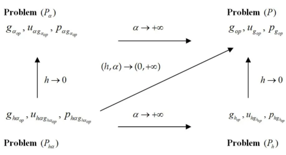
Theorem 1

We have the following complete commutative diagram which relates the continu-ous distributed mixed optimal control problems

( )

P

_α and

( )

P

, with the discrete dis-tributed mixed optimal control problems

(

P

hα

)

and

( )

P

h and it is obtained by taking the limits h→0,α →+∞ and

( , )

h

α →

(0,

+

∞

)

, as in Figure 1, where

g

hα_op,

h op

h g

u

α

α and

p

h gα h opα are respectively the optimal control, the system and the adjoint system states of the discrete distributed mixed optimal control problem

(

P

hα

)

for each

0

h> and α >0, and the double convergence is the diagonal one.

Fig. 1. Relationship among optimal control problems

₍

Phα

_{) ( ) ( )}

, Pα , Ph and ( )P by taking the

limits h→0, α→+∞ and ( , )hα →(0,+∞).

The study of the limit h→0 of the discrete solutions of optimal control

problems can be considered as a classical limit, see [4-6, 8, 9, 13-15, 19, 23, 24, 27, 28] but the limit α →+∞, for each h>0, and the double limit

( , )

h

α →

(0,

+

∞

)

can be considered as a new ones.

The paper is organized as follows. In Section II we define the discrete elliptic variational equalities for the state systems _uhg and

α

h g

u , we define the discrete dis-tributed cost functional J_h and

J

_hα, we define the discrete distributed optimal control problems

( )

P

h and

(

P

hα

)

, and the discrete elliptic variational equalities for the

ad-joint state systems p_hg and p_{h gα} for each h>0 and α >0, and we obtain properties

for the discrete optimal control problems

( )

P

h and

(

P

hα

)

. In Section III we study the

classical convergences of the discrete distributed optimal control problems

( )

P

h to

( )

P

, and

(

P

hα

)

to

( )

P

α when h→0 (for each α>0) and the estimations for the

discrete cost functional J_h and α h

J

. In Section IV we study the new convergence of the discrete distributed optimal control problems

(

P

_hα

)

to

( )

P

_h when

_α

→

+

∞

for each

h

>

0

and we obtain a commutative diagram which relates the continuous and discrete distributed mixed optimal control problems

₍

Phα

_{) ( ) ( )}

, Pα , Ph and

( )

P

by taking the limits h→0 and α →+∞. In Section V we study the new double

conver-gence of the discrete distributed optimal control problems

(

P

hα

)

to

( )

P

when

α →

+

∞

( , )

h

(0,

)

and we obtain the diagonal convergence in the previous commuta-tive diagram.

2

Discretization by Finite Element Method and Properties

We consider the finite element method and a polygonal domain n

Ω ⊂R with a regular triangulation with Lagrange triangles of type 1, constituted by affine-equivalent finite element of class _C0 _{being h the parameter of the finite element} approximation which goes to zero [3, 7]. We can take h equal to the longest side of the triangles

T

∈

τ

_h and we can approximate the sets

V V

,

0

and

K

by:

( )

( )

{

0

}

{

}

1 0 1 0 / , , / 0 ; h h h h h h h h h h V = v ∈C Ω v T P T∈ ∀ ∈T τ V = v ∈V v Γ = K = +b V (14)

where P₁ is the set of the polymonials of degree less than or equal to 1. Let 0

: ( )

h C Vh

π

Ω → be the corresponding linear interpolation operator. Then there exists

a constant

c

₀

>

0

(independent of the parameter h) such that [3]:

( )

( )

1

( )

0 0 ) r ; ) r ; r ,1 2 h H r h V r a v

π

v c h v b v

π

v c h− v v H r − ≤ − ≤ ∀ ∈ Ω < ≤ . (15)

We define the discrete cost functional J J_h, _hα:H ₀+

→R by the following expressions:

( )

1 2 2

( )

1 2 2 ) , ) 2 2 2 2 h hg d H H h h g d H H M M a J g = u −z + g b J_α g = u_α −z + g (16)

where u_hg and u_{h gα} are the discrete system states defined as the solution of the fol-lowing discrete elliptic variational equalities [16, 24]:

(

)

(

)

2 0 : , , , hg h hg h h h h h u K a u v g v qv d

_γ

v V Γ ∈ = −

_∫

∀ ∈ , (17)

(

)

(

)

2 1 : , , , h g h h g h h h h h h u_α V a u_{α α} v g v qv d

_{γ α}

bv d

_γ

v V Γ Γ ∈ = −

_∫

+

_∫

∀ ∈ . (18)

The corresponding discrete distributed optimal control problems consists in finding gh_op,ghα_op∈Hsuch that:

( )

( )

(

)

( )

) Problem ( ) : , ) Problem ( ) : op op h h h _{g H} h h h h _{g H} h a P J g Min J g b P_α J_α g_α Min J_α g ∈ ∈ = = (19)

and their corresponding discrete adjoint states p_hg and p_{h gα} are defined respectively as the solution of the following discrete elliptic variational equalities:

(

) (

)

0 : , , , 0 hg h hg h hg d h h h p ∈V a p v = u −z v ∀ ∈v V (20)

(

) (

)

: , , , h g h h g h h g d h h h p_α ∈V a_α p_α v = u_α −z v ∀ ∈v V (21)

Remark 1. We note that the discrete (in the n-dimensional space) distributed opti-mal control problem (P_h) and (

P

_hα) are still infinite dimensional optimal control problems since the control space is not discretized.

Lemma 2

(i) There exist unique solutions u_hg∈K_h and p_hg∈V_0h, and u_{h gα} ∈V_h and

h g h

p_α ∈V of the elliptic variational equalities (17) and (20), (18), and (21)

respec-tively ∀ ∈g H, ∀ ∈q Q,

b

>

0

on

Γ

₁.

(ii) The operators g H∈ →u_hg∈V, and g H∈ →uh gα ∈V are Lipschitzians.

The operators g H∈ →p_hg∈V_0g, and g H∈ → ph gα ∈Vh are Lipschitzians and

strictly monotone operators.

Proof. We use the Lax-Milgram Theorem, the variational equalities (17), (18), (20) and (21), the coerciveness (10) and (11) and following [10, 18, 25].

W

Theorem 3

(i) The discrete cost functional

J

_h and

J

_hαare H- elliptic and strictly convexe applications, that is

₍

∀g g_{1, 2}∈H,∀ ∈t

_{[ ]}

0,1

₎

:

(

) ( )

( )

(

(

)

)

(

)

2 2 1 1 2 2 1 1 1- 1 2 h h h H t t t J g +tJ g −J tg + −t g ≥M − g −g (22)

(

)

( )

2

( )

1

(

1

(

)

2

)

(

)

2 1 2 1 1- 1 2 h h h H t t t J_α g +tJ_α g −J_α tg + −t g ≥M − g −g (23)

(ii) There exist a unique optimal controls

op

h

g ∈H and ghα_op∈H that satisfy the

optimization problems (19a) and (19b) respectively.

(iii)

J

_h and

J

_hα are Gâteaux differenciable applications and their derivatives are given by the following expressions:

( )

( )

) h hg, ) h h g, , 0

a J gʹ =Mg p+ b Jʹ_α g =Mg p+ _α ∀ ∈g H ∀h> (24)

(iv) The optimality condition for the optimization problems (19a) and (19b) are given by:

( )

1

(

)

1 a) 0 ; b) 0 op op hop op op hop h h h hg h h h h g J g g p J g g p M α α α M α α ʹ = ⇔ =− ʹ = ⇔ =− (25)

(v) J_hʹ and

J

_h

ʹ

_α are Lipschitzians and strictly monotone operators.

Proof. We use the definitions (16a,b), the elliptic variational equalities (17) and (18) and the coerciveness (10) and (11), following [10,18,25].

W

We define the operators:

( )

1

( )

1 , : such that a) , ) h h h hg h h g W W H H W g p b W g p M M α → =− α =− α . (26) Theorem 4 We have that:

(i) W_h and

W

_hα are Lipschitzian operators, and W_h (

W

_hα) is a contraction opera-tor if and only if M is large, that is:

2 2

1 1

a) M > , b) M >

α

λ

λ

. (27)

(ii) If M verifies the inequalities (27a,b) then the discrete distributional optimal control

op

h

g ∈H (ghαop∈H) is obtained as the unique fixed point of Wh (

W

hα), i.e.:

( )

(

)

1 1 , op hop op op op hop op op h hg h h h h h g h h h g p W g g g p W g g M α M α α α α α =− ⇔ = =− ⇔ = . (28)

Proof. We use the definitions (26a,b), and the properties (25a,b) and Lemma 2.

W

3

Convergence of the Discrete Distributed Optimal Control

Problems

_{( )}

P

_h

to

_{( )}

P

and

₍

P

_hα

₎

to

_{( )}

P

_α

when

h

→

0

We obtain the following error estimations between the continuous and discrete solutions:

Theorem 6

We suppose the continuous system states and adjoint system states have the regu-larities ,

_{( )}

op r g g u u H α α ∈ Ω and , op

( )

r g g p p H α α ∈ Ω

(

1<r≤2

)

. If M verifies the

1_, 1_, 1 op op hop op hop op r r r h _H hg g hg g V V g ₋g _≤ch − u ₋u _≤ch− p ₋p _≤ch − ₍₂₉₎ 1_, 1_, 1 op op hop op hop op r r r h _H h g g h g g V V g g ch u u ch p p ch α α α α α α α α α α − − − − ≤ − ≤ − ≤ (30)

where c’s are constants independents of h.

Proof. It is useful to use the restriction α >1 by splitting aαby [21, 24,25]

(

)

(

)

1 1 , , ( 1) a u v_α a u v

α

uvd

γ

Γ = + −

_∫

(31)

but then it can be replaced by

_{α α}

_≥

₀ for any

α

₀

>

0

. We follow a similar method to

the one developed in [25] for Neumann boundary optimal control problems by using the elliptic variational equalities (17), (18), (20) and (21), the thesis holds.

W

Remark 2. If M verifies the inequalities (27a,b) we can obtain the convergence in Theorem 6 by using the characterization of the fixed point (28a,b), and the uniqueness of the optimal controls g_op∈H and gα_op∈H.

Now, we give some estimations for the discrete cost functional

J

_hα and J_h.

Lemma 7 If M verifies the inequality (27a,b)and the continuous system states and adjoint system states have the regularities , r

_{( )}

g g

u u_α ∈H Ω p pg, αg∈Hr

_{( )}

Ω

(

1<r≤2

)

then we have the following error bonds:

( ) ( )

(

)

( )

2 2 2( 1)_, 2( 1) 2 hop op op op 2 hop op op op r r h h H H M M g g J g J g Ch g_α gα J gα α J gα α Ch − − − ≤ − ≤ − ≤ − ≤ (32)

( )

( )

( )

( )

2 2 2( 1)_; 2( 1) 2 hop op op hop 2 hop op op hop r r h h h h H H M M g g J g J g Ch g_α gα Jα gα Jα g_α Ch − − − ≤ − ≤ − ≤ − ≤ (33)

( ) ( )

1_,

( ) ( )

1 op op op op r r h h h J g J g Ch− J g J g Ch− − ≤ − ≤ (34)

( )

( )

1_,

(

)

( )

1 op op op op r r h h h J_α g J g_α Ch− J_α g_α J g_{α α} Ch− − ≤ − ≤ (35)

where C’s are constants independents of h and α .

Proof. Estimations (32) and (33) follow from the estimations (29), and the equali-ties (similar relationship for

J

and

J

_α):

(

hop

)

( )

op 1₂ h ghop gop 2_{H 2} hop op 2_H

M

J g J g u u g g

α α

( )

op

( )

hop 12 hop hop 2 2 hop op 2 h h h g h g H H M J g J g u u g g α α α α α − α = α − α + − α (37)

( )

( )

1 , 2 h h g g _H g d _H h g g _H J_α g −J_α g ≤_⎜⎛ u_α −u_α + u_α −z ⎞_⎟ u_α −u_α ∀ ∈g H ⎝ ⎠ .

W

(38)

4

Convergence of the Discrete Optimal Control Problems

₍

P

_hα

₎

to

_{( )}

P

_h

when

α

→

+

∞

Theorem 9

We have the following limits:

lim _{h h} lim _{h h} lim _{op op} 0 , 0

op op op op h g hg h g hg h h _H V V u u p p g g h α α α α α α→+∞ − =α→+∞ − =α→+∞ − = ∀ > . (39)

Proof. We omit this proof because we prefer to prove the next one with more de-tails.

5

Double Convergence of the Discrete Distributed Optimal

Control Problem

₍

P

_hα

₎

to

_{( )}

P

when

_{( , )}

_h

_α

_→

_(0,

₊

_∞

₎

For the discrete distributed optimal control problem

₍

P_hα

₎

we will now con-sider the double limit

( , )

h

_{α →}

(0,

₊

_∞

)

.

Theorem 10

We have the following limits:

( , ) (0,h_αlim_{→ +∞})uh gαhαop−ugop V =( , ) (0,h_αlim_{→ +∞}) ph gαhαop−pgop V =( , ) (0,h_αlim_{→ +∞}) ghαop−gop H =0 (40)

Proof. From now on we consider that c’s represent positive constants independ-ents simultaneously of h>0 and α >0 (see (31)). We show a sketch of the proof by obtaining the following estimations (for ∀h>0 and ∀α >1):

(

) (

)

1 2 0 1, 0 2, 1 0 3 h V h V h u c u_α c

α

u_α b d

γ

c Γ ≤ ≤ −

_∫

− ≤ (41) 4, 5, 6 op hop op h h g h H H H g c u c g c α α ≤ α ≤ ≤ (42)

(

)

(

)

1 2 7, 8, 1 9 hop hop hop hg h g h g V V u c u c u b d c α α α

α

α

γ

Γ ≤ ≤ −

_∫

− ≤ (43)

(

)

1 2 10, 11, 1 12 hop hop hop hg h g h g V V p c p c p d c α α α

α

α

γ

Γ ≤ ≤ −

_∫

≤ . (44)

For example, the constant c₁₁is a positive constant independent simultaneously of

0

h> and α >0, and it is given by the following expression:

11 1 1 1 1 1 1 1 1 0 2 2 1 1 1 1 1 1 1 1 1 1 1 1 1 1 1 1 1 1 1 1 1 1 1 1 1 1 1 1 1 1 1 1 1 1 1 1 1 1 1 1 1 d H Q c z M M b M M M q M λ λ λ λλ λ λ λ λ λ λ λ λ λ λ γ λ λ λ λ λλ λ λ λ λ ⎡ ⎛ ⎛ ⎞⎞ ⎛ ⎞⎛ ⎞⎤ = ⎢ _⎜⎜ + ⎜ + + ⎟⎟_⎟+ ⎜ + ⎟⎜ + ⎟⎥ ⎝ ⎠ ⎢ ⎝ ⎝ ⎠⎠ ⎝ ⎠ ⎥ ⎣ ⎦ ⎡ ⎛ ⎞⎛ ⎞ ⎛ ⎞⎛ ⎞⎤ + ⎢ ⎜ + ⎟_⎜⎜ + + ⎟_⎟+ ⎜ + ⎟⎜ + ⎟⎥ ⎝ ⎠ ⎢ ⎝ ⎠⎝ ⎠ ⎝ ⎠ ⎥ ⎣ ⎦ ⎛ ⎞ ⎛ ⎞ ⎛ ⎞ + + ⎜ + ⎟+ + ⎜ + ⎟+ ⎜ + ⎝ ⎠ ⎝ ⎠ ⎝ ⎠ 2 1 1 1 1 1 1 M λ λ λ ⎡ ⎡ ⎛ ⎞⎤ ⎛ ⎞⎛ ⎞⎤ ⎢ ⎢ ⎜⎜ ⎟⎟⎟⎥+ ⎜ + ⎟⎜ + ⎟⎥ ⎢ ⎢⎣ ⎝ ⎠⎥⎦ ⎝ ⎠⎝ ⎠⎥ ⎣ ⎦ (45)

Therefore, from the above estimations we have that:

/ in weak as ( , ) (0, ) op h f H g_α f H h

α

∃ ∈ ⎯⎯→ → +∞ (46) 1

/ in weak ( strong) as ( , ) (0, ) with /

h op h g V u V H h b α α

η

η

α

η

∃ ∈ ⎯⎯→ → +∞ Γ = (47) 1 / in weak ( strong) as ( , ) (0, ) with / 0

h op h g V p V H h α α

ξ

ξ

α

ξ

∃ ∈ ⎯⎯→ → +∞ Γ = (48) / in weak as op h h h f H g_α f H

α

∃ ∈ ⎯⎯→ →+∞ (49) 1 / in weak (in strong) as with /

h op

h V uh gα _α h V H h b

η

η

α

η

∃ ∈ ⎯⎯→ →+∞ Γ = (50)

1

/ in weak (in strong) as with / 0

h op h V ph gα _α h V H h

ξ

ξ

α

ξ

∃ ∈ ⎯⎯→ →+∞ Γ = (51) / in weak as 0 op h f_α H g_α f_α H h ∃ ∈ ⎯⎯→ → (52) 1

/ in weak (in strong) as 0 with /

h op h g V u V H h b α α α α α

η

η

η

∃ ∈ ⎯⎯→ → Γ = (53) 1

/ in weak (in strong) as 0 with / 0

h op h g V p V H h α α α α α

ξ

ξ

ξ

∃ ∈ ⎯⎯→ → Γ = (54) * _/ * _{in weak as 0} op h f H g f H h ∃ ∈ ⎯⎯→ → (55) * * * 1 / in weak ( strong) as 0 with /

hop hg V u V H h b

η

η

η

∃ ∈ ⎯⎯→ → Γ = (56) * * * 1

/ in weak ( strong) as 0 with / 0

hop hg

V p V H h

ξ

ξ

ξ

Taking into account the uniqueness of the distributed optimal control problems

(

Phα

) ( ) ( )

, Pα , Ph and

( )

P , and the uniqueness of the elliptic variational equalities corresponding to their state systems we get

, , h hop h hop hop h uhf uhg h phf phg fh g

η

= =

ξ

= = = (58) , , op op op f g f g u u p p f g α α α α α α α α α α α α

η

= =

ξ

= = = (59) * _, * _, * op op op f g f g u u p p f f g

η η

= = =

ξ ξ

= = = = = . (60)

Now, by using [11] we obtain

lim _op 0, lim 0, lim 0

op op

g g

H V V

f_α g _α u _α p

α→+∞ − = α→+∞

η

− = α→+∞

ξ

− = (61)

and therefore the three double limits (40) hold when

( , )

h

_{α →}

(0,

₊

_∞

)

.

Proof of Theorem 1. It is a consequence of the properties (29), (30), (39), (40) and [10,11].

Remark 3. We note that this double convergence is a novelty with respect to the recent results obtained for a family of discrete Neumann boundary optimal control problems [25].

Acknowledgements

The present work has been partially sponsored by the Projects PIP No 0534 from CONICET - Univ. Austral, Rosario, Argentina, and AFOSR-SOARD Grant FA9550-14-1-0122.

References

1. Azzam, A., Kreyszig, E.: On solutions of elliptic equations satisfying mixed boundary conditions. SIAM J. Math. Anal. 13, 254-262 (1982).

2. Bergounioux, M.:Optimal control of an obstacle problem. Appl. Math. Optim. 36,

147-172 (1997).

3. Brenner, S., Scott, L.R.: The mathematical theory of finite element methods. Springer, New York (2008).

4. Casas, E., Mateos, M.: Uniform convergence of the FEM. Applications to state constrained control problems. Comput. Appl. Math. 21, 67-100 (2002).

5. Casas, E., Mateos, M.: Dirichlet contol problems in smooth and nonsmooth convex plain domains. Control Cybernetics. 40, 931-955 (2011).

6. Casas, E., Raymond, J.P.: Error estimates for the numerical approximation of Dirichlet boundary control for semilinear elliptic equations. SIAM J. Control Optim. 45, 1586-1611 (2006).

8. Deckelnick, K, Günther, A., Hinze, M.: Finite element approximation of ellliptic control problems with constraints on the gradient. Numer. Math. 111, 335-350 (2009).

9. Deckelnick, K., Hinze, M.: Convergence of a finite element approximation to a state-constrained ellliptic control problem. SIAM J. Numer. Anal. 45, 1937-1953 (2007). 10. Gariboldi, C.M., Tarzia, D.A.: Convergence of distributed optimal controls on the internal

energy in mixed elliptic problems when the heat transfer coefficient goes to infinity. Appl. Math. Optim. 47, 213-230 (2003).

11. Gariboldi, C.M., Tarzia, D.A.: A new proof of the convergence of the distributed optimal controls on the internal energy in mixed elliptic problems. MAT – Serie A. 7, 31-42 (2004).

12. Haller-Dintelmann, R., Meyer, C., Rehberg, J., Schiela, A.: Hölder continuity and optimal control for nonsmooth elliptic problems. Appl. Math. Optim. 60, 397-428 (2009).

13. Hintermüller, M., Hinze, M.: Moreau-Yosida regularization in state constrained ellliptic control problems: Error estimates and parameter adjustement. SIAM J. Numer. Anal. 47, 1666-1683 (2009).

14. Hinze, M.: A variational discretization concept in control constrained optimization: The linear-quadratic case. Comput. Optim. Appl. 30, 45-61 (2005).

15. Hinze, M., Matthes, U.: A note on variational dicretization of elliptic Nuemann boundary control. Control Cybernetics. 38, 577-591 (2009).

16. Kinderlehrer, D., Stampacchia, G.: An introduction to variational inequalities and their ap-plications. SIAM, Philadelphia (2000).

17. Lanzani, L., Capogna, L., Brown, R.M.: The mixed problem in Lpfor some two-dimensional Lipschitz domain. Math. Annalen.342,91-124(2008).

18. Lions, J.L. : Contrôle optimal des systèmes gouvernés par des équations aux dérivées par-tielles. Dunod, Paris (1968).

19. Mermri, E.B., Han, W.: Numerical approximation of a unilateral obstacle problem. J. Op-tim. Th. Appl. 153, 177-194 (2012).

20. Shamir, E.: Regularization of mixed second order elliptic problems. Israel J. Math. 6, 150-168 (1968).

21. Tabacman, E.D., Tarzia, D.A.: Sufficient and/or necessary condition for the heat transfer coefficient on Γ₁and the heat flux on Γ₂ to obtain a steady-state two-phase Stefan prob-lem. J. Diff. Eq. 77, 16-37 (1989).

22. Tarzia, D.A.: An inequality for the constant heat flux to obtain a steady-state two-phase Stefan problem. Eng. Anal. 5, 177-181 (1988).

23. Tarzia, D.A.: Numerical analysis for the heat flux in a mixed elliptic problem to obtain a discrete steady-state two-phase Stefan problem. SIAM J. Numer. Anal. 33, 1257-1265 (1996).

24. Tarzia, D.A.: Numerical analysis of a mixed elliptic problem with flux and convective boundary conditions to obtain a discrete solution of non-constant sign. Numer. Meth. PDE. 15, 355-369 (1999).

25. Tarzia, D.A.: A commutative diagram among discrete and continuous boundary optimal control problems. Adv. Diff. Eq. Control Processes. 14, 23-54 (2014).

26. Tröltzsch, F.: Optimal control of partial differential equations. Theory, methods and appli-cations. American Mathematical Society. Providence (2010).

27. Yan, M., Chang, L., Yan, N.: Finite element method for constrained optimal control prob-lems governed by nonlinear elliptic PDEs. Math. Control Related Fields. 2, 183-194 (2012).

28. Ye, Y., Chan, C.K., Lee, H.W.J.: The existence results for obstacle optimal control prob-lems. Appl. Math. Comput. 214, 451-456 (2009).