We provide the following resources online at compstorylab.org/share/papers/dodds2014a/ and at

(1)

We provide the following resources online at http://

compstorylab.org/share/papers/dodds2014a/and at

http://hedonometer.org.

• Links to example scripts for parsing and measuring average happiness scores for texts, and for gener-ating D3 word shifts: http://compstorylab.org/ share/papers/dodds2014a/code.html

• Visualizations for exploring translation-stable word pairs across languages;

• Interactive, multi-language time series for over 10,000 works of literature including Moby Dick and Harry Potter;

• Jellyfish plots for all 24 corpora;

• An API for selected data streams and word lists at

http://hedonometer.org/api.html

• Spatiotemporal hedonometric measurements of Twitter across all 10 languages, explorable at http://hedonometer.org.

Corpora

We used the services of Appen Butler Hill (http:

//www.appen.com) for all word evaluations excluding

English, for which we had earlier employed Mechanical Turk (https://www.mturk.com/[17]).

English instructions (see the example below) were translated to all other languages and given to partici-pants along with survey questions, and an example of the English instruction page is below. Non-english language experiments were conducted through a custom interac-tive website built by Appen Butler Hill, and all partici-pants were required to pass a stringent aural proficiency test in their own language.

100 individual words on a 9 point unhappy-happy scale.

Please consider each word carefully. If we determine that your ratings are randomly or otherwise inappropriately selected, or that any questions are left unanswered, we may not approve your work. These words were chosen based on their common usage. As a result, a small portion of words may be offensive to some people, written in a different language, or nonsensical.

Before completing the word ratings, we ask that you answer a few short demographic questions. We expect the entire survey to require 10 minutes of your time. Thank you for participating!

Example:

sunshine

Read the word and click on the face that best corresponds to your emotional response.

Demographic Questions 1. What is your gender? (Male/Female) 2. What is your age? (Free text)

3. Which of the following best describes your highest achieved education level? Some High School, High School Graduate, Some college, no degree, Associates degree, Bachelors degree, Graduate degree (Masters, Doctorate, etc.) 4. What is the total income of your household?

5. Where are you from originally? 6. Where do you live currently?

7. Is your first language? (Yes/No) If it is not, please specify what your first language is.

(2)

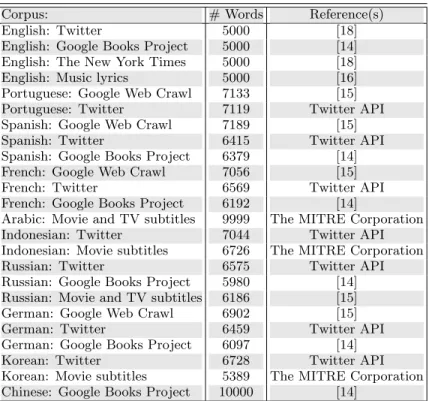
Corpus: # Words Reference(s)

English: Twitter 5000 [18]

English: Google Books Project 5000 [14]

English: The New York Times 5000 [18]

English: Music lyrics 5000 [16]

Portuguese: Google Web Crawl 7133 [15]

Portuguese: Twitter 7119 Twitter API

Spanish: Google Web Crawl 7189 [15]

Spanish: Twitter 6415 Twitter API

Spanish: Google Books Project 6379 [14]

French: Google Web Crawl 7056 [15]

French: Twitter 6569 Twitter API

French: Google Books Project 6192 [14]

Arabic: Movie and TV subtitles 9999 The MITRE Corporation

Indonesian: Twitter 7044 Twitter API

Indonesian: Movie subtitles 6726 The MITRE Corporation

Russian: Twitter 6575 Twitter API

Russian: Google Books Project 5980 [14]

Russian: Movie and TV subtitles 6186 [15]

German: Google Web Crawl 6902 [15]

German: Twitter 6459 Twitter API

German: Google Books Project 6097 [14]

Korean: Twitter 6728 Twitter API

Korean: Movie subtitles 5389 The MITRE Corporation

Chinese: Google Books Project 10000 [14]

TABLE S1. Sources for all corpora.

Language Participants’ location(s) Number of participants Average words scored

English United States of America, India 384 1302

German Germany 196 2551 Indonesian Indonesia 146 3425 Russian Russia 125 4000 Arabic Egypt 185 2703 French France 179 2793 Spanish Mexico 236 2119 Portuguese Brazil 208 2404

Simplified Chinese China 128 3906

Korean Korea, United States of America 109 4587

TABLE S2. Number and main country/countries of location for participants evaluating the 10,000 common words for each of the 10 languages we studied. Also recorded is the average number of words evaluated by each participant (rounded to the nearest integer). We note that each word received 50 evaluations from distinct individuals. The English word list was evaluated via Mechanical Turk for our initial study [17]. The nine languages evaluated through Appen-Butler Hill yielded a higher participation rate likely due to better pay and the organization’s quality of service.

(3)

1 2 3 4 5 6 7 8 9

h

avg

Russian: Google Books

Chinese: Google Books

German: Google Web Crawl

Korean: Twitter

German: Google Books

Korean: Movie subtitles

French: Google Web Crawl

German: Twitter

Portuguese: Google Web Crawl

Spanish: Google Web Crawl

Russian: Twitter

French: Google Books

Indonesian: Twitter

French: Twitter

Russian: Movie and TV subtitles

Indonesian: Movie subtitles

Spanish: Google Books

English: Google Books

Arabic: Movie and TV subtitles

English: New York Times

English: Twitter

English: Music Lyrics

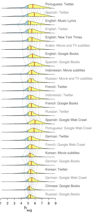
FIG. S1. The same average happiness distributions shown in Fig. 1 re-ordered by increasing variance. Yellow indicates above neutral (havg= 5), blue below neutral, red vertical lines mark each distribution’s median, and the gray background lines connect the deciles of adjacent distributions.

(4)

Spanish Portuguese English Indonesian French German Arabic Russian Korean Chinese Spanish 1.00, 0.00 1.01, 0.03 1.06, -0.07 1.22, -0.88 1.11, -0.24 1.22, -0.84 1.13, -0.22 1.31, -1.16 1.60, -2.73 1.58, -2.30 Portuguese 0.99, -0.03 1.00, 0.00 1.04, -0.03 1.22, -0.97 1.11, -0.33 1.21, -0.86 1.09, -0.08 1.26, -0.95 1.62, -2.92 1.58, -2.39 English 0.94, 0.06 0.96, 0.03 1.00, 0.00 1.13, -0.66 1.06, -0.23 1.16, -0.75 1.05, -0.10 1.21, -0.91 1.51, -2.53 1.47, -2.10 Indonesian 0.82, 0.72 0.82, 0.80 0.88, 0.58 1.00, 0.00 0.92, 0.48 0.99, 0.06 0.89, 0.71 1.02, 0.04 1.31, -1.53 1.33, -1.42 French 0.90, 0.22 0.90, 0.30 0.94, 0.22 1.09, -0.52 1.00, 0.00 1.08, -0.44 0.99, 0.12 1.12, -0.50 1.37, -1.88 1.40, -1.77 German 0.82, 0.69 0.83, 0.71 0.86, 0.65 1.01, -0.06 0.92, 0.41 1.00, 0.00 0.91, 0.61 1.07, -0.25 1.29, -1.44 1.32, -1.36 Arabic 0.88, 0.19 0.92, 0.08 0.95, 0.10 1.12, -0.80 1.01, -0.12 1.10, -0.68 1.00, 0.00 1.12, -0.63 1.40, -2.14 1.43, -2.01 Russian 0.76, 0.88 0.80, 0.75 0.83, 0.75 0.98, -0.04 0.89, 0.45 0.93, 0.24 0.89, 0.56 1.00, 0.00 1.26, -1.39 1.25, -1.05 Korean 0.62, 1.70 0.62, 1.81 0.66, 1.67 0.77, 1.17 0.73, 1.37 0.78, 1.12 0.71, 1.53 0.79, 1.10 1.00, 0.00 0.98, 0.28 Chinese 0.63, 1.46 0.63, 1.51 0.68, 1.43 0.75, 1.07 0.71, 1.26 0.76, 1.03 0.70, 1.41 0.80, 0.84 1.02, -0.29 1.00, 0.00 TABLE S3. Reduced Major Axis (RMA) regression fits for row language as a linear function of the column language: h(row)avg (w) =

mh(column)avg (w) +cwhere windicates a translation-stable word. Each entry in the table contains the coefficient pairmandc. See the scatter plot tableau of Fig. 2 for further details on all language-language comparisons. We use RMA regression, also known as Standardized Major Axis linear regression, because of its accommodation of errors in both variables.

Spanish Portuguese English Indonesian French German Arabic Russian Korean Chinese

Spanish 1.00 0.89 0.87 0.82 0.86 0.82 0.83 0.73 0.79 0.79 Portuguese 0.89 1.00 0.87 0.82 0.84 0.81 0.84 0.84 0.79 0.76 English 0.87 0.87 1.00 0.88 0.86 0.82 0.86 0.87 0.82 0.81 Indonesian 0.82 0.82 0.88 1.00 0.79 0.77 0.83 0.85 0.79 0.77 French 0.86 0.84 0.86 0.79 1.00 0.84 0.77 0.84 0.79 0.76 German 0.82 0.81 0.82 0.77 0.84 1.00 0.76 0.80 0.73 0.74 Arabic 0.83 0.84 0.86 0.83 0.77 0.76 1.00 0.83 0.79 0.80 Russian 0.73 0.84 0.87 0.85 0.84 0.80 0.83 1.00 0.80 0.82 Korean 0.79 0.79 0.82 0.79 0.79 0.73 0.79 0.80 1.00 0.81 Chinese 0.79 0.76 0.81 0.77 0.76 0.74 0.80 0.82 0.81 1.00

TABLE S4. Pearson correlation coefficients for translation-stable words for all language pairs. Allp-values are<10−118_{. These}

values are included in Fig. 2 and reproduced here for to facilitate comparison.

Spanish Portuguese English Indonesian French German Arabic Russian Korean Chinese

Spanish 1.00 0.85 0.83 0.77 0.81 0.77 0.75 0.74 0.74 0.68 Portuguese 0.85 1.00 0.83 0.77 0.78 0.77 0.77 0.81 0.75 0.66 English 0.83 0.83 1.00 0.82 0.80 0.78 0.78 0.81 0.75 0.70 Indonesian 0.77 0.77 0.82 1.00 0.72 0.72 0.76 0.77 0.71 0.71 French 0.81 0.78 0.80 0.72 1.00 0.80 0.67 0.79 0.71 0.64 German 0.77 0.77 0.78 0.72 0.80 1.00 0.69 0.76 0.64 0.62 Arabic 0.75 0.77 0.78 0.76 0.67 0.69 1.00 0.74 0.69 0.68 Russian 0.74 0.81 0.81 0.77 0.79 0.76 0.74 1.00 0.70 0.66 Korean 0.74 0.75 0.75 0.71 0.71 0.64 0.69 0.70 1.00 0.71 Chinese 0.68 0.66 0.70 0.71 0.64 0.62 0.68 0.66 0.71 1.00

(5)

Portuguese: Google Web Crawl -0.085 6.33×10−13 _{-0.060 3.23} ×10−7 _-3.98 ×10−5 _5.96 Portuguese: Twitter -0.041 5.98×10−4 _{-0.030 1.15} ×10−2 _-2.40 ×10−5 _5.73

English: Google Books -0.042 3.03×10−3 _{-0.013 3.50}

×10−1 _-3.04

×10−5 _5.62

English: New York Times -0.056 6.93×10−5 _{-0.044 1.99}_×₁₀−3 _-4.17_×₁₀−5 _5.61

German: Google Web Crawl -0.096 1.11×10−15 _{-0.082 6.75}_×₁₀−12 _-3.67_×₁₀−5 _5.65

French: Google Web Crawl -0.105 9.20×10−19 _{-0.080 1.99}

×10−11 _-4.50

×10−5 _5.68

English: Twitter -0.097 6.56×10−12 _{-0.103 2.37}

×10−13 _-7.78

×10−5 _5.67

Indonesian: Movie subtitles -0.039 1.48×10−3 _{-0.063 2.45}

×10−7 _-2.04

×10−5 _5.45

German: Twitter -0.054 1.47×10−5 _{-0.036 4.02}_×₁₀−3 _-2.51_×₁₀−5 _5.58

Russian: Twitter -0.052 2.38×10−5 _{-0.028 2.42}_×₁₀−2 _-2.55_×₁₀−5 _5.52

French: Google Books -0.043 6.80×10−4 _{-0.030 1.71}

×10−2 _-2.31

×10−5 _5.49

German: Google Books -0.003 8.12×10−1 _{+0.014 2.74}

×10−1 _-1.38

×10−6 _5.45

French: Twitter -0.049 6.08×10−5 _{-0.023 6.31}

×10−2 _-2.54

×10−5 _5.54

Russian: Movie and TV subtitles -0.029 2.36×10−2 _{-0.033 9.17}_×₁₀−3 _-1.57_×₁₀−5 _5.43

Arabic: Movie and TV subtitles -0.045 7.10×10−6 _{-0.029 4.19}_×₁₀−3 _-1.66_×₁₀−5 _5.44

Indonesian: Twitter -0.051 2.14×10−5 _{-0.018 1.24} ×10−1 _-2.50 ×10−5 _5.46 Korean: Twitter -0.032 8.29×10−3 _{-0.016 1.91} ×10−1 _-1.24 ×10−5 _5.38

Russian: Google Books +0.030 2.09×10−2 _{+0.070 5.08}

×10−8 _+1.20

×10−5 _5.35

English: Music Lyrics -0.073 2.53×10−7 _{-0.081 1.05}_×₁₀−8 _-6.12_×₁₀−5 _5.45

Korean: Movie subtitles -0.187 8.22×10−44 _{-0.180 2.01}_×₁₀−40 _-9.66_×₁₀−5 _5.41

Chinese: Google Books -0.067 1.48×10−11 _{-0.050 5.01}

×10−7 _-1.72

×10−5 _5.21

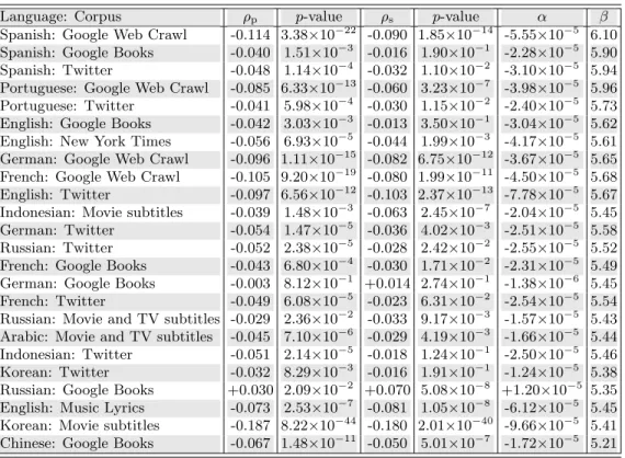
TABLE S6. Pearson correlation coefficients andp-values, Spearman correlation coefficients andp-values, and linear fit coeffi-cients, for average word happinesshavg as a function of word usage frequency rankr. We use the fit ishavg=αr+β for the most common 5000 words in each corpora, determiningαandβvia ordinary least squares, and order languages by the median of their average word happiness scores (descending). We note that stemming of words may affect these estimates.

Language: Corpus ρp p-value ρs p-value α β

Portuguese: Twitter +0.090 2.55×10−14 _{+0.095 1.28} ×10−15 _1.19 ×10−5 _1.29 Spanish: Twitter +0.097 8.45×10−15 _{+0.104 5.92} ×10−17 _1.47 ×10−5 _1.26

English: Music Lyrics +0.129 4.87×10−20 _{+0.134 1.63}_×₁₀−21 _2.76_×₁₀−5 _1.33

English: Twitter +0.007 6.26×10−1 _{+0.012 4.11}_×₁₀−1 _1.47_×₁₀−6 _1.35

English: New York Times +0.050 4.56×10−4 _{+0.044 1.91}_×₁₀−3 _9.34_×₁₀−6 _1.32

Arabic: Movie and TV subtitles +0.101 7.13×10−24 _{+0.101 3.41}

×10−24 _9.41

×10−6 _1.01

English: Google Books +0.180 1.68×10−37 _{+0.176 4.96}

×10−36 _3.36

×10−5 _1.27

Spanish: Google Books +0.066 1.23×10−7 _{+0.062 6.53}_×₁₀−7 _9.17_×₁₀−6 _1.26

Indonesian: Movie subtitles +0.026 3.43×10−2 _{+0.027 2.81}_×₁₀−2 _2.87_×₁₀−6 _1.12

Russian: Movie and TV subtitles +0.083 7.60×10−11 _{+0.075 3.28}_×₁₀−9 _1.06_×₁₀−5 _0.89

French: Twitter +0.072 4.77×10−9 _{+0.076 8.94} ×10−10 _1.07 ×10−5 _1.05 Indonesian: Twitter +0.072 1.17×10−9 _{+0.072 1.73} ×10−9 _8.16 ×10−6 _1.12

French: Google Books +0.090 1.02×10−12 _{+0.085 1.67}_×₁₀−11 _1.25_×₁₀−5 _1.02

Russian: Twitter +0.055 6.83×10−6 _{+0.053 1.67}_×₁₀−5 _7.39_×₁₀−6 _0.91

Spanish: Google Web Crawl +0.119 4.45×10−24 _{+0.106 2.60}_×₁₀−19 _1.45_×₁₀−5 _1.23

Portuguese: Google Web Crawl +0.093 4.06×10−15 _{+0.083 2.91}

×10−12 _1.07

×10−5 _1.26

German: Twitter +0.051 4.45×10−5 _{+0.050 5.15}

×10−5 _7.39

×10−6 _1.15

French: Google Web Crawl +0.104 2.12×10−18 _{+0.088 9.64}_×₁₀−14 _1.27_×₁₀−5 _1.01

Korean: Movie subtitles +0.171 1.39×10−36 _{+0.185 8.85}_×₁₀−43 _2.58_×₁₀−5 _0.88

German: Google Books +0.157 6.06×10−35 _{+0.162 4.96}_×₁₀−37 _2.17_×₁₀−5 _1.03

Korean: Twitter +0.056 4.07×10−6 _{+0.062 4.25}

×10−7 _6.98

×10−6 _0.93

German: Google Web Crawl +0.099 2.05×10−16 _{+0.085 1.18}

×10−12 _1.20

×10−5 _1.07

Chinese: Google Books +0.099 3.07×10−23 _{+0.097 3.81}_×₁₀−22 _8.70_×₁₀−6 _1.16

Russian: Google Books +0.187 5.15×10−48 _{+0.177 2.24}_×₁₀−43 _2.28_×₁₀−5 _0.81

TABLE S7. Pearson correlation coefficients andp-values, Spearman correlation coefficients andp-values, and linear fit coef-ficients for standard deviation of word happiness hstd as a function of word usage frequency rankr. We consider the fit is

hstd=αr+β for the most common 5000 words in each corpora, determining αandβ via ordinary least squares, and order corpora according to their emotional variance (descending).

(6)

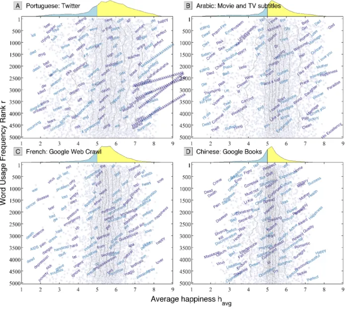
FIG. S2. Reproduction of Fig. 3 in the main text with words directly translated into English using Google Translate. Note that the instances of “kkkkk ...” for Brazilian Portuguese are left unchanged by Google Translate but should be interpreted as “hahahhaha ...”. See the caption of Fig. 3 for details.

(7)

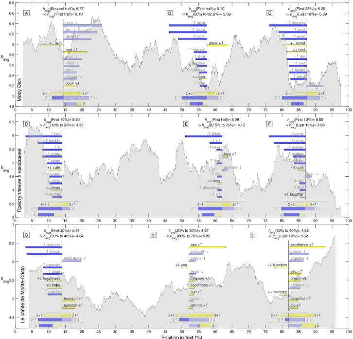
FIG. S3. Fig. 4 from the main text with Russian and French translated into English. Online, interactive visualizations of over 10,000 books can be found here: http://hedonometer.org/books.html.

(8)

0.2 0.4 0.6 0.8 1 1.2 1.4 1.6 1.8 2 x 105 5 5.2 5.4 5.6 5.8 6 6.2 6.4 6.6 Word n u mb e r i ha v g

Moby Dic k, ∆h=2.0, s mooth in g T=10000

Moby Dic k ( Ran d omize d ) , ∆h=2.0, s mooth in g T=10000

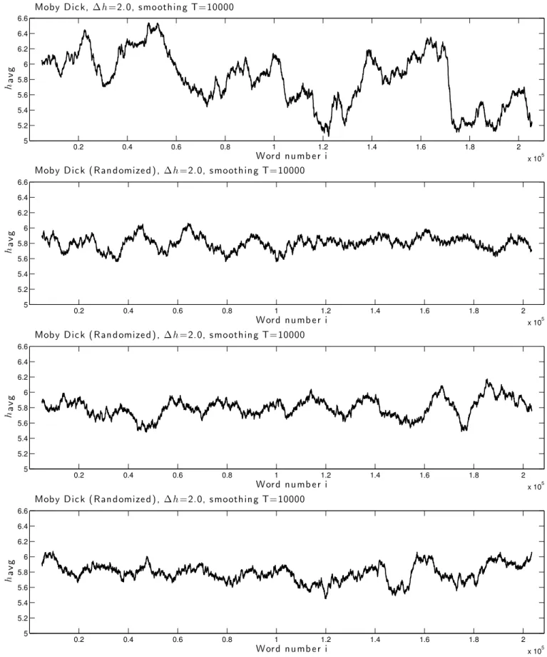
FIG. S4. Comparison of the emotional trajectory of Moby Dick with the results for three example randomized versions of the same text, showing the loss of structure and variability.

(9)

Figs. 4 and S3. We expand upon the approach described in [16] and [18] to rank and visualize how words con-tribute to this overall upward shift in happiness.

Shown below is the third inset word shift used in Fig 4 for the Count of Monte Cristo, a comparison of words found in the last 10% of the book (Tcomp, havg = 6.32) relative to those used between 30% and 40% (Tref, havg = 4.82). For this particular measurement, we employed the ‘word lens’ which excluded words with 3< havg<7.

We will use the following probability notation for the normalized frequency of a given wordwin a textT:

Pr(w|T;L) = P f(w|T;L)

w′∈Lf(w′|T;L)

, (1)

where f(w|T;L) is the frequency of word w in T with word lens L applied [16]. (For the example word shift above, we haveL={[1,3],[7,9]}.) We then estimate the happiness score of any textT as

havg(T;L) =X

w∈L

havg(w)Pr(w|T;L), (2)

where havg(w) is the average happiness score of a word as determined by our survey.

We can now express the happiness difference between = w∈L havg(w)Pr(w|Tcomp;L)− w∈L havg(w)Pr(w|Tref;L) =X w∈L

havg(w) [Pr(w|Tcomp;L)−Pr(w|Tref;L)]

=X

w∈L

[havg(w)−havg(Tref;L)]

×[Pr(w|Tcomp;L)−Pr(w|Tref;L)],

(3) where we have introducedhavg(Tref;L) as base reference for the average happiness of a word by noting that

X

w∈L

havg(Tref;L) [Pr(w|Tcomp;L)−Pr(w|Tref;L)] =havg(Tref;L)X

w∈L

[Pr(w|Tcomp;L)−Pr(w|Tref;L)]

=havg(Tref;L) [1−1] = 0. (4) We can now see the change in average happiness between a reference and comparison text as depending on how these two quantities behave for each word:

δh(w) = [havg(w)−havg(Tref;L)] (5)

and

δp(w) = [Pr(w|Tcomp;L)−Pr(w|Tref;L)]. (6)

Words can contribute to or work against a shift in average happiness in four possible ways which we encode with symbols and colors:

• δh(w) >0, δp(w) >0: Words that are more

pos-itive than the reference text’s overall average and are used more in the comparison text (+↑, strong yellow).

• δh(w)<0, δp(w)<0: Words that are less positive

than the reference text’s overall average but are used less in the comparison text (−↓, pale blue). • δh(w)>0, δp(w)<0: Words that are more

posi-tive than the reference text’s overall average but are used less in the comparison text (+↓, pale yellow). • δh(w) <0, δp(w) >0: Words that are more

pos-itive than the reference text’s overall average and are used more in the comparison text (−↑, strong blue).

Regardless of usage changes, yellow indicates a relatively positive word, blue a negative one. The stronger colors indicate words with the most simple impact: relatively positive or negative words being used more overall.

We order words by the absolute value of their contri-bution to or against the overall shift, and normalize them as percentages.

(10)

Simple Word Shifts

For simple inset word shifts, we show the 10 top words in terms of their absolute contribution to the shift.

Returning to the inset word shift above, we see that an increase in the abundance of relatively positive words ‘excellence’ ‘mer’ and ‘rêve’ (+↑, strong yellow) as well as a decrease in the relatively negative words ‘prison’ and ‘prisonnier’ (−↓, pale blue) most strongly contribute to the increase in positivity. Some words go against this trend, and in the abbreviated word shift we see less usage of relatively positive words ‘liberté’ and ‘été’ (+↓, pale

yellow).

The normalized sum total of each of the four categories of words is shown in the summary bars at the bottom of the word shift. For example, Σ+↑ represents the total shift due to all relatively positive words that are more prevalent in the comparison text. The smallest contri-bution comes from relatively negative words being used more (−↑, strong blue).

The bottom bar with Σ shows the overall shift with a breakdown of how relatively positive and negative words separately contribute. For the Count of Monte Cristo example, we observe an overall use of relatively positive words and a drop in the use of relatively negative ones (strong yellow and pale blue).