Available online throug
ISSN 2229 – 5046
A NOTE ON POLYNOMIAL INTERPOLATION FORMULAE
1
Ramesh Kumar Muthumalai* and G. Uthra
21
Department of Mathematics, Saveetha Engineering College, Thandalam, Chennai-602105, India.
2
Department of Mathematics, Pachaiyappa's College
,
Chennai- 600030, India.
(Received On: 22-06-14; Revised & Accepted On: 30-07-14)
ABSTRACT
T
hrough introducing a formula for divided difference and new schemes of divided difference tables, we study an interpolation formula, which generalizes both Newton and Lagrange interpolation formula to use interpolants that fit the derivatives, as well as the function values for arbitrary spaced grids. Using this, we derive other interpolation formulas, in terms of differences and divided differences for evenly spaced data. Comparing with former polynomial interpolation formulas, these new formulas have some new featured advantages for approximating functional values for evenly and unevenly spaced data.AMS subject Classification: 65D05.
Key words: Divided difference; Interpolation; Hermite Interpolation;
1. INTRODUCTION
Polynomial Interpolation theory has a number of important uses. Its primary use is to furnish some mathematical tools that are used in developing methods in the areas of approximation theory, numerical integration and the numerical solution of differential equations [1]. A number of different methods have been developed to construct useful interpolation formulas for evenly and unevenly spaced points. Newton’s divided difference formula [1, 3] and Lagrange’s formula [2, 4, 5] are the most popular interpolation formulas for polynomial interpolation to any arbitrary degree with finite number of points.
Lagrange interpolation is a well known, classical technique for interpolation. Using this; one can generate a single polynomial expression which passes through every point given. This requires no additional information about the points. This can be really bad in some cases, as for large numbers of points we get very high degree polynomials which tend to oscillate violently, especially if the points are not so close together. Newton's formula for constructing the interpolation polynomial makes the use of divided differences through Newton’s divided difference table for unevenly spaced data [1]. Based on this formula, there exists many number of interpolation formulas using differences through difference table, for evenly spaced data. The best formula is chosen by speed of convergence, but each formula converges faster than other under certain situations, no other formula is preferable in all cases. For example, if the interpolated value is closer to the center of the table then we go for any one of central difference formulas, (Gauss’s, Stirling’s and Bessel’s etc) depending on the value of argument position from the center of the table [7]. However, Newton interpolation formula is easier for hand computation but Lagrange interpolation formula is easier when it comes to computer programming. In this paper, we study a new interpolation formula which generalizes both Newton and Lagrange interpolation formula with new scheme of divided difference tables for evenly and unevenly spaced data. Also, we study the comparisons of new interpolation formulas with the former interpolation formulas based on differences.
Corresponding author:
1Ramesh Kumar Muthumalai*
2.1. New Divided Difference Table
In Newton divided difference table, divided differences of new entries in each column are determined by divided difference of two neighboring entries in the previous column. But, the procedure of new divided difference table is different from the Newton divided difference table. For example, consider the argument values
x
0,
x
1,
x
2
,
x
6 for the corresponding functional valuesf
0,
f
1,
f
2,
,
f
6. As a matter of convenience, we write fk = f(xk). The procedure of New divided difference table is given in Table 1. The first order divided differences in the third column of the Table 1 are found by the sequence of evaluatingf
[
x
0,
x
1]
,f
[
x
0,
x
2],
, The second order divided differences in the fourth column of the Table 1 are found by the sequence of evaluatingf
[
x
0,
x
1,
x
2]
,
],
,
,
[
x
0x
1x
3f
. Similarly, the sequencesf
[
x
0,
x
1,
x
2,
x
3]
,f
[
x
0,
x
1,
x
2,
x
4],
are evaluated for fifth column and the sequencesf
[
x
0,
x
1,
x
2,
x
3,
x
4]
,f
[
x
0,
x
1,
x
2,
x
3,
x
5]
are evaluated for sixth column and so on.2.2. Combined form of Newton divided difference Table and New divided difference Table
Here, Newton divided difference table and new divided difference table are combined to produce a new combined form of divided difference table as shown in the Table 2. For example, consider the argument values
x
0,
x
1,
x
2
,
x
6 for the corresponding functional valuesf
0,
f
1,
f
2,
,
f
6. The table is divided into two parts and separated by a crossed line. The first part contains first four data follows the procedure of Newton divided difference table and remaining follows the procedure of new divided difference table.Table 1: New divided difference table Table 2: Combined form of Newton
divided difference Table and New divided difference Table
x y δ1 δ2 δ3 δ4 x y δ1 δ2 δ3 δ4
0
x f0 x0 f0
f[x0,x1] f[x0,x1]
1
x f1 f[x0,x1,x2] x1 f1 f[x0,x1,x2] f[x0,x2] f[x0,x1,x2,x3] f[x1,x2] f[x0,x1,x2,x3]
2
x f2 f[x0,x1,x3] f[x0,x1,x2,x3,x4] x2 f2 f[x1,x2,x3] f[x0,x1,x2,x3,x4]
f[x0,x3] f[x0,x1,x2,x4] f[x2,x3] f[x1,x2,x3,x4] 3
x f3 f[x0,x1,x4] f[x0,x1,x2,x3,x5] x3 f3 f[x2,x3,x4] f[x0,x1,x2,x3,x5]
f[x0,x4] f[x0,x1,x2,x5] f[x3,x4] f[x0,x1,x2,x5]
4
x f4 f[x0,x1,x5] f[x0,x1,x2,x3,x6] x4 f4 f[x0,x1,x5] f[x0,x1,x2,x3,x6]
f[x0,x5] f[x0,x1,x2,x6] f[x0,x5] f[x0,x1,x2,x6]
5
x f5 f[x0,x1,x6] x5 f5 f[x0,x1,x6]
f[x0,x6] f[x0,x6] 6
x f6 x6 f6
2.3. Table of differences and divided differences by integer arguments.
Suppose the data are evenly spaced then, the construction of difference table is easier than new divided difference table. So, we have to change procedure of new combined form of divided difference table. Let
h
a
h
a
h
a
Table 3: Table of differences and divided differences by Integer Table 4: Table of central differences and divided differences.
Arguments
x y δ1 δ2 δ3 δ4 x y δ1 δ2 δ3 δ4
0 f0 −2 f−2
! 1 0 f ∆
δf−2
1 f1
! 2
0 2f
∆ -1
1
−
f δ2f−2
∆f1
! 3
0 3
f
∆
! 1 1
−
f
δ
! 3
2 3
−
f
δ
2 f2 ∆2f1 ! 4
0 4f
∆ 0
0
f
! 2
1 2
−
f
δ ! 4
2 4
−
f
δ
∆f2 ∆3f1 ! 1 0 f
δ
! 3
1 3
−
f
δ
3 f3 ∆2f2 fI[0,1,2,3,5] 1 f1 δ2f0 fI[0,−1,1,−2,3]
∆f3 fI[0,1,2,5] δf1 fI[0,−1,1.3]
4 f4 fI[0,1,5] fI[0,1,2,3,6] 2 f2 fI[0,−1,3] fI[0,−1,1,−2,4]
fI[0,5] fI[0,1,2,6] fI[0,3] fI[0,−1,14]
5 f5 fI[0,1,6] 3 f3 fI[0,−1,4]
fI[0,6] fI[0,6]
6 f6 4 f4
Algorithm 2.1: (New Divided difference table). Given the first two columns of the table, containing
x
0,
x
1,
,
x
n and, correspondinglyf
[
x
0],
f
[
x
1],
,
f
[
x
n]
, then the remaining entries are generated by the following steps,Step-1: For i = 1 to r do
Step-2: For j = 0 to n-i do
Step-3:
[
,
,
,
,
,
] [
,
,
,
,
,
]
[
,
,
,
,
,
]
.
1
1 2 2
1 0 2
2 1 0 1
2 1 0
− +
− − +
− +
−
−
−
=
i j i
i i j
i i j
i i
x
x
x
x
x
x
x
f
x
x
x
x
x
f
x
x
x
x
x
f
Algorithm 2.2: (Combined form of divided difference table) Given the first two columns of the table, containing
n
x
x
x
0,
1,
,
and, correspondinglyf
[
x
0],
f
[
x
1],
,
f
[
x
n]
, then the remaining entries are generated by the following steps,Step-1: For i = 1 to r do
Step-2: For j = 0 to n-i do
Step-3: If j < r-i+1 then
[
,
1,
2,
,
] [
1,
2,
3,
,
] [
,
1,
2,
,
1]
.
j i j
j i j
j j i
j j
j j i
j j
j j
x
x
x
x
x
x
f
x
x
x
x
f
x
x
x
x
f
−
−
=
+
− + +
+ +
+ + + +
+
+
Otherwise
[
,
,
,
,
,
] [
,
,
,
,
,
]
[
,
,
,
,
,
]
.
1
1 2 2
1 0 2
2 1 0 1
2 1 0
− +
− − +
− +
−
−
−
=
i j i
i i j
i i j
i i
x
x
x
x
x
x
x
f
x
x
x
x
x
f
x
x
x
x
x
f
3. INTERPOLATION FORMULAS
Theorem 3.1: Let x0,x1,xr−1 are ‘r’ numbers and xr,xr+1,,xn are (n−r+1) distinct numbers on the interval ]
,
.
)
(
)!
1
(
)
(
]
,
,
,
,
[
)
(
)
(
]
,
,
,
[
)
(
0 ) 1 ( 1 1 0 1 0 1 0 1 1 0 0∏
∏
∑
∏
∏
∑
= + ≠= − = − = − = − =−
+
+
−
−
−
+
−
=
n i i n n j i rj i j j r n r i i r i i i j j i r i
x
x
n
f
x
x
x
x
x
x
x
x
f
x
x
x
x
x
x
x
f
x
f
ξ
(3.1)Proof: Using Newton’s interpolation formula on
x
0,
x
1,
x
r−1, we have].
,
,
,
,
[
)
(
)
)(
(
]
,
,
,
[
)
(
)
)(
)(
(
]
,
,
[
)
)(
(
]
,
[
)
(
)
(
)
(
1 1 0 1 1 0 1 2 1 0 2 2 1 0 2 1 0 1 0 1 0 0 0 − − − −−
−
−
+
−
−
−
−
+
+
−
−
+
−
+
=
r r r rx
x
x
x
f
x
x
x
x
x
x
x
x
x
x
f
x
x
x
x
x
x
x
x
x
x
x
f
x
x
x
x
x
x
f
x
x
x
f
x
f
(3.2)Using formula for divided difference polynomial found in Ref [6]
[
,
0,
1,
,
1]
∑
[
,
0,
1,
,
1]
∏
[
,
0,
1,
,
]
∏
(
)
.
= ≠= = − −
−
+
−
−
=
n r i i n n j i rj i j j n r i r i
r
f
x
x
x
x
x
x
x
x
x
x
x
x
x
x
f
x
x
x
x
f
(3.3)Substituting above equation (3.2) in (3.3), then
0 0 0 1 0 1 2 0 1 1
( 1) 1
0 1 1
0 0
( )
( ) (
) [ , ]
(
)(
)
(
) [ , ,
,
]
( )
(
)
[ ,
, ,
,
]
(
).
(
1)!
r r nr n n n
j
i i r i
i r
i i r i j i
i j
f x
f x
x
x
f x x
x
x
x
x
x
x
f x x
x
x
x
f
x
x
f x x x
x
x
x
x
x
n
ξ
− − + − − = = = = ≠=
+ −
+ + −
−
−
−
+
−
+
−
−
+
∑
∏
∏
∏
After simplification, we obtain (3.1).
Remark 3.2: If we put
r
=
n
andr
=
0
in Theorem 3.1, we obtain Newton’s general nterpolation formula and Lagrange’s interpolation formula respectively.Remark 3.3: The following are some difference formulas for equally spaced points derived using various interpolation formulas.
(i) Let
x
0,
x
1,
x
2
x
n are (n+1) distinct numbers on the interval[
a
,
b
]
, spaced equally i.ex
i=
x
0+
ih
,
(
i
=
0
,
1
,
2
,
n
)
, h≠0 andf
∈
C
n+1[
a
,
b
]
, ifx
=
x
0+
sh
,
then[
]
(
).
)!
1
(
1
,
,
1
,
0
,
!
)
(
( 1)) 1 ( 1 ) ( 1 1 ) ( 0 0 0
ξ
+ + + = ≠= − =+
+
−
−
−
+
∆
+
=
+
∑
∑
n∏
n n nr i n j i r j I r r i i i
f
n
s
h
j
i
j
s
r
i
f
s
i
s
f
f
sh
x
f
(3.4)where ∆if0 is the ith difference and fI
[
i,0,1,,r−1]
is the thr divided difference by integer arguments
(ii). Let
x
0,
x
1,
x
2
x
n are(
n
+
1
)
distinct numbers on the interval[
a
,
b
]
,x
∈
[
a
,
b
]
spaced equally i.e,)
,
2
,
1
,
0
(
,
0
ih
i
n
x
x
i=
−
=
,h
≠
0
andf
∈
C
n+1[
a
,
b
]
, ifx
=
x
0+
sh
,
then[
]
( ) 1 ( 1) ( 1)
1 ( ) 0 0 0 1
( )
(
)
( 1)
, 0, 1,
, (
1)
.
!
(
1)!
i i n n n n
r n
r n r
I
i i r j r
i j
f s
s
j
h
s
f
f x
sh
f
s
f
i
r
i
i
j
n
ξ
− + − − + − − − = = = ≠∇
+
+
=
+
+
−
−
−
− −
+
−
+
∑
∑
∏
(3.5)Where
∇
if
0 isi
thbackward difference andf
I[
−
i
,
0
,
−
1
,
,
−
r
−
1
]
isr
th divided difference by integer arguments(iii). Let
x
−m
x
−2,
x
−1,x
0,
x
1,
x
2
x
n are the(
n
+
m
+
1
)
distinct numbers on the interval[a,b],x
∈
[
a
,
b
]
spaced equally, i.e.
x
i=
x
0+
ih
,
(
i
=
−
m
,
,
−
2
,
−
1
,
0
,
1
,
2
,
n
)
,h
≠
0
andf
∈
C
n+m+1[
a
,
b
]
, if,
0
sh
x
.
)
(
)!
1
(
)
(
]
,
,
2
,
2
,
1
,
1
,
0
,
[
)
(
)
1
(
!
2
)
1
(
!
3
!
2
!
1
)
(
) 1 ( 1 , ) 1 ( , ) 1 ( ) 1 2 ( ) 2 ( 2 ) 3 ( 1 3 ) 2 ( 1 2 ) 1 ( 0 1 0 0∏
∏
∑
− = + + + + + − ≠ + ± = + − + ± = + − − −−
+
+
+
−
−
−
−
−
+
+
−
+
+
+
+
+
+
+
=
+
n m i m n m n n m j i r j n m r i I r r r ri
s
m
n
f
h
j
i
j
s
r
r
i
f
r
s
r
s
r
f
s
f
s
f
s
f
f
sh
x
f
ξ
δ
δ
δ
δ
(3.6).
)
(
)!
1
(
)
(
]
,
,
,
1
,
1
,
0
,
[
)
(
)
(
!
2
)
1
(
!
3
)
1
(
!
2
!
1
)
(
) 1 ( 1 , ) 1 ( , ) 1 ( ) 1 2 ( ) 2 ( 2 ) 3 ( 2 3 ) 2 ( 1 2 1 1 0 0∏
∏
∑
− = + + + + − ≠ + ± = − + ± = + − − − −−
+
+
+
−
−
−
−
+
+
+
+
+
+
+
+
+
+
=
+
n m i m n m n n m j i r j n m r i I r r r ri
s
m
n
f
h
j
i
j
s
r
r
i
f
r
s
r
s
r
f
s
f
s
f
s
f
f
sh
x
f
ξ
δ
δ
δ
δ
(3.7)(3.6) and (3.7) are new central difference forward and backward difference formula respectively.
Remark 3.4: Let
∑
∏
+ − ≠=± + + − + ± = +
−
−
−
−
−
+
=
Θ
m nj i r j n m r i I r
j
i
j
s
r
r
i
f
r
s
s
, ) 1 ( , ) 1 ( ) 1 2 (]
,
,
,
2
,
2
,
1
,
1
,
0
,
[
)
(
)
(
and∏
− = + + + + + +=
+
+
−
n m i n m n m nm
s
i
n
m
f
h
R
(
)
)!
1
(
)
(
) 1 ( 1 1ξ
.Using Theorem 3.1, we can improve Striling’s, Bessels’s, Everett’s and Steffensen’s central difference formulas as follows .
.
)
(
!
2
)
1
(
)
(
!
1
2
)
1
(
2
)
(
)
1
(
)
1
(
!
2
!
1
2
)
1
(
)
0
(
)
(
1 ) 1 2 ( 2 ) 1 2 ( 1 2 1 2 2 2 1 1 0 0 + + − − − −+
Θ
+
−
+
−
+
−
−
+
−
+
+
−
+
+
−
+
−
+
+
=
+
m n r r r r rR
s
r
r
s
s
r
f
r
r
s
r
f
r
f
f
s
s
f
f
f
sh
x
f
δ
δ
δ
δ
δ
δ
(3.8).
)
(
2
)
(
!
2
)
1
(
2
)
1
(
)
(
!
2
)
1
(
)
1
(
!
3
)
1
(
)
(
2
)
0
(
)
1
(
!
2
)
1
(
)
0
(
!
1
)
(
2
)
(
1 1 2 ) 2 ( 2 2 ) 2 ( 3 2 1 2 2 2 1 1 0 0 + + ++
Θ
+
−
−
+
+
+
−
+
−
−
+
+
−
−
−
+
+
−
−
+
−
+
+
=
+
m n r r r r rR
s
r
f
r
r
s
r
f
r
f
r
r
s
f
s
s
s
f
f
s
s
f
s
f
f
sh
x
f
δ
δ
δ
δ
δ
δ
δ
(3.9).
)
(
)
1
(
!
2
)
(
)
0
(
!
3
)
1
(
)
1
(
!
1
2
)
1
(
)
1
(
!
3
)
1
(
)
(
1 ) 2 ( 2 2 ) 3 ( 1 ) 1 2 ( 2 2 2 ) 3 ( 0 0 + + − −+
Θ
+
−
+
−
+
+
+
+
+
+
−
+
−
+
−
+
+
−
+
+
=
+
m n r r r rR
s
r
s
r
r
f
f
s
s
f
r
t
r
r
f
f
t
t
f
sh
x
f
δ
δ
δ
δ
(3.10) and.
)
(
)
1
(
!
2
)
(
!
2
)
(
)
1
(
!
2
)
1
(
!
2
)
1
(
)
0
(
)
(
1 ) 2 ( 1 2 ) 2 ( 1 2 ) 2 ( ) 2 ( 0 0 + + − −+
Θ
+
−
+
−
−
+
+
−
+
+
−
−
+
+
=
+
m n r r r rR
s
r
s
r
r
f
r
r
s
r
f
s
f
s
f
f
sh
x
f
δ
δ
δ
δ
(3.11)where
t
=
1
-
s
, Equations (3.8)-(3-11) are new modified form of Striling’s, Bessels’s, Everett’s and Steffensen’s central difference formulas respectively.4. APPROXIMATION BY NEW INTERPOLATION FORMULA
The general structure of the new interpolation formula can be written in the following form
)
(
)
(
)
(
)
)(
)(
(
)
(
)
(
x
N
x
x
x
x
x
x
x
x
x
x
E
x
where
f
0,
f
1,
f
2,
,
f
n are the functional values of the function f, for the distinct argumentsx
0,
x
1,
x
2
x
n andf
∈
C
n+1[
a
,
b
]
. N(x) is Newton’s interpolation formula up to certain order andλ
(
x
)
is the divided difference polynomial. To approximate new interpolation formula, we can replaceλ
(
x
)
by a suitable approximationΠ
(
x
)
. We can use least squares or any other methods to replaceλ
(
x
)
byΠ
(
x
).
i.e.
f
(
x
)
=
N
(
x
)
+
(
x
−
x
0)(
x
−
x
1)(
x
−
x
2)
(
x
−
x
r−1)
Π
(
x
).
(4.2))
(
x
Π
is an approximation of rthdivided difference polynomial, obtained from the new divided difference table. The replacement of Π(x) by the suitable approximation is shown through an example. Here, we use Method of least squares to replaceΠ
(
x
)
. The actual function taken for comparison is f(x)=ex(1+x)+xsinx and the argument values x and corresponding functional values y are given in the following table.Table - 5
x 1.0 1.25 1.5 1.75 2.0 2.25 2.5 2.75 3.00
y 6.2780346 9.0395024 12.7004652 17.5471328 23.9857632 32.5858062 44.1349092 59.7094373 80.7655077
In this example,, former formulas of interpolation based on differences are compared by their speed of convergence. We consider the 4th the degree polynomial, generated by Newton forward and backward, Gauss forward and backward, Stirling’s, Bessel’s, Everett’s and Steffensen’s interpolation formulas. The errors of various interpolation formulas with actual functional values on (0.85, 3.15) are shown in the Table 6. Similarly, The new modified formulas (of Newton forward and backward, Gauss forward and backward, etc) are used to calculate 4th degree polynomial. The divided difference polynomial is replaced by the function
θ
(s)
, whereθ
(s)
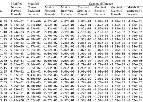
is a linear function found by using method of least squares, on 3rd order divided differences generated in the new divided difference table. The errors of various new interpolation formulas and their actual functional values on (0.85, 3.15) are shown in the Table 7.Newton forward and backward formulas give fair accuracy near the beginning and end of the Table 6 respectively. But, at the central zone of Table 6, central difference formulas give fair accuracy than Newton forward and backward formulas. But, comparing the results of corresponding former formulas in Table 6 to new modified formulas in Table 7, it is clear that the new modified formulas give better accuracy than the former formulas. Through out the interval (0.85, 3.15) new modified formulas possess better accuracy.
Table - 6: Errors by Newton forward and backward, Gauss forward and backward, etc., with actual function values on some values of x
Newton Newton Central difference
x Forward Backward Forward Backward Strirling’s Bessel’s Everett’s Steffensen’s Formula Formula Formula Formula formula formula formula formula
3.00 -2.78e+00 0.00e+00 -4.44e-01 -4.44e-01 -4.44e-01 -2.67e-01 -4.44e-01 -4.44e-01 3.10 -3.99e+00 -1.93e-02 -7.80e-01 -7.80e-01 -7.80e-01 -4.95e-01 -7.80e-01 -7.80e-01 3.15 -4.74e+00 -4.00e-02 -1.01e+00 -1.01e+00 -1.01e+00 -6.56e-01 -1.01e+00 -1.01e+00
Table – 7: Errors by equations (3.5) to (3.11) with actual functional values on various values of x
Modified Modified Cenntral difference
Newton Newton Modified Modified Modified Modified Modified Modified x Forward Backward Forward Backward Strirling’s Bessel’s Everett’s Steffensen’s Formula Formula Formula Formula Formula Formula Formula Formula
0.85 3.00e-02 1.71e+00 4.87e-01 4.87e-01 4.87e-01 4.87e-01 4.87e-01 4.87e-01 0.90 1.52e-02 1.31e+00 3.62e-01 3.62e-01 3.62e-01 3.62e-01 3.62e-01 3.62e-01 1.00 0.00e+00 6.93e-01 1.82e-01 1.82e-01 1.82e-01 1.82e-01 1.82e-01 1.82e-01 1.10 -3.24e-03 2.77e-01 7.19e-02 7.19e-02 7.19e-02 7.19e-02 7.19e-02 7.19e-02 1.15 -2.61e-03 1.29e-01 3.70e-02 3.70e-02 3.70e-02 3.70e-02 3.70e-02 3.70e-02 1.25 0.00e+00 -6.88e-02 -3.91e-03 -3.91e-03 -3.91e-03 -3.91e-03 -3.91e-03 -3.91e-03 1.35 1.78e-03 -1.68e-01 -1.86e-02 -1.86e-02 -1.86e-02 -1.86e-02 -1.86e-02 -1.86e-02 1.50 0.00e+00 -1.97e-01 -1.58e-02 -1.58e-02 -1.58e-02 -1.58e-02 -1.58e-02 -1.58e-02 1.65 -5.61e-03 -1.51e-01 -5.02e-03 -5.02e-03 -5.02e-03 -5.02e-03 -5.02e-03 -5.02e-03 1.75 -8.49e-03 -1.06e-01 0.00e+00 0.00e+00 0.00e+00 0.00e+00 0.00e+00 0.00e+00 1.85 -7.79e-03 -6.21e-02 1.81e-03 1.81e-03 1.81e-03 1.81e-03 1.81e-03 1.81e-03 2.00 5.19e-03 -1.28e-02 0.00e+00 0.00e+00 0.00e+00 0.00e+00 0.00e+00 0.00e+00 2.10 2.41e-02 5.54e-03 -1.70e-03 -1.70e-03 -1.70e-03 -1.70e-03 -1.70e-03 -1.70e-03 2.15 3.68e-02 1.05e-02 -1.93e-03 -1.93e-03 -1.93e-03 -1.93e-03 -1.93e-03 -1.93e-03 2.25 6.77e-02 1.33e-02 0.00e+00 0.00e+00 0.00e+00 0.00e+00 0.00e+00 0.00e+00 2.35 1.03e-01 9.43e-03 5.85e-03 5.85e-03 5.85e-03 5.85e-03 5.85e-03 5.85e-03 2.50 1.47e-01 0.00e+00 2.01e-02 2.01e-02 2.01e-02 2.01e-02 2.01e-02 2.01e-02 2.65 1.42e-01 -3.45e-03 2.78e-02 2.78e-02 2.78e-02 2.78e-02 2.78e-02 2.78e-02 2.75 7.99e-02 0.00e+00 1.40e-02 1.40e-02 1.40e-02 1.40e-02 1.40e-02 1.40e-02 2.85 -6.32e-02 5.46e-03 -3.36e-02 -3.36e-02 -3.36e-02 -3.36e-02 -3.36e-02 -3.36e-02 3.00 -5.15e-01 0.00e+00 -2.22e-01 -2.22e-01 -2.22e-01 -2.22e-01 -2.22e-01 -2.22e-01 3.10 -1.05e+00 -3.48e-02 -4.75e-01 -4.75e-01 -4.75e-01 -4.75e-01 -4.75e-01 -4.75e-01 3.15 -1.41e+00 -7.02e-02 -6.57e-01 -6.57e-01 -6.57e-01 -6.57e-01 -6.57e-01 -6.57e-01
Table - 8: Comparisons of Total number of different operations of various interpolation formulas.
5. CONCLUSION
The new interpolation formula which generalizes both Newton’s and Lagrange’s interpolation formulas has been studied in this paper by introducing a new formula of divided difference and new schemes of divided difference tables.
Further, we study other new interpolation formulas based on the differences and divided differences. Also comparisons of former interpolation formulas (Newton’s, Gauss’s, Stirling, Bessel’s, etc.,) with the new modified formulas are shown that the new formulas are very efficient and posses good accuracy for evaluating functional values between given data. Comparison table (Table 8) in section 4 shows the new interpolation formula is superior to Newton’s and Lagrange’s interpolation formulas.
REFERENCES
[1] Atkinson A. E, An Introduction to Numerical Analysis, 2 Ed., John Wiley & Sons, New York, 1989.
[2] Burden R. L, Faires J. D, Numerical Analysis, seventh ed., Brooks/Cole, Pacific Grove, CA, 2001. Operations Newton divided difference
Formula
Lagrange Interpolation formula
New Interpolation formula, Theorem 3.1 n
r<
<
0
Additions n n n
Subtractions 3n(n+1)/2 2n(n+1) n(n+1)+(n−r)(n−r+1)+r(r+1)/2 Multiplications n(n+1)/2 (2n−1)(n+1) (2(n−r)−1)(n−r+1)+r(r+1)/2
[3] Conte S.D, Carl de Boor, Elementary Numerical Analysis, 3 Ed, McGraw-Hill, New York, USA, 1980.
[4]
S
u
li
E, and Mayers. D, An Introduction to Numerical Analysis, Cambridge, UK, 2003.[5] Mathews J. H , Fink K. D, Numerical methods using MATLAB, 4ed, Pearson Education, USA, 2004
[6] R.K. Muthumalai, Some formulas for numerical differentiation of through divided differences, Int. Jour. Math. Arch (IJMA), Vol 3(10), 2012, 1-4.
[7] Scarborough J. B, Numerical Mathematical Analysis, 6 Ed, The John Hopkins Press, USA, 1966.
Source of support: Nil, Conflict of interest: None Declared