Proceedings of the
Seventh International Workshop on
Graph Transformation and Visual Modeling Techniques
(GT-VMT 2008)
Foundations of Modelling and Simulation of Complex Systems
Hans Vangheluwe
12 pages
Guest Editors: Claudia Ermel, Reiko Heckel, Juan de Lara
Managing Editors: Tiziana Margaria, Julia Padberg, Gabriele Taentzer
Foundations of Modelling and Simulation of Complex Systems
Hans Vangheluwe
School of Computer Science McGill University, Qu´ebec, Canada
Abstract: Modelling and simulation are becoming increasingly important enablers for the analysis and design of complex systems. In application domains such as automotive design, the notion of a “virtual experiment” is taken to the limit and complex designs are model-checked, simulated, and optimized extensively before a single realization is ever made. This “doing it right the first time” leads to tremen-dous cost savings and improved quality. Furthermore, with appropriate models, it is often possible to automatically synthesize (parts of) the system-to-be-built.
In this paper, the basic concepts of modelling and simulation are introduced. These concepts are based on general systems theory and start from the idea of a model as an abstract representation of knowledge about structure and behaviour of some system. The purpose is either analysis or design in a particular experimental context.
Typically, different formalisms are used such as Ordinary Differential Equations, Queueing Networks, and State Automata. It will be shown how these different for-malisms all share a common structure and differ in the choice of time base, state space, and description of temporal evolution. This allows one to classify formalisms on the one hand and to find a common ground for implementing simulators on the other hand.
Keywords:modelling, simulation, systems theory, multi-formalism
1
Introduction
Real-World entity
Base Model
System S
only study behaviour in experimental context
experiment within context
Model M
Simulation Results Experiment
Observed Data
within context
simulate
= virtual experiment
Model Base a-priori knowledge
validation
REALITY MODEL
GOALS
Modelling and Simulation Process
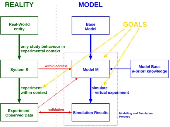
Figure 1: Modelling and simulation concepts
Often, an iterative combination of analysis and design is needed to solve real problems. Though the focus of modelling and simulation is on the time-varying behaviour of dynamical systems, static systems are a limit-case. Both physical (obeying conservation and constraint laws) and non-physical (informational, such as software) systems and their interactions are studied.
This paper first introduces the general concepts of Modelling and Simulation theory. The rep-resentation of models in diverse formalisms, at different levels of abstraction, and the behaviour-conserving transformation between the formalisms is discussed. Multi-formalism model repre-sentation is presented as an enabler for open, distributed, modelling and simulation systems.
2
Modelling and Simulation Basics
2.1 Concepts
Figure1presents modelling and simulation concepts as introduced by Zeigler [ZPK00].
Object is some entity in the Real World. Such an object can exhibit widely varying behaviour depending on the context in which it is studied as well as the aspects of its behaviour which are under study.
Base Model is a hypothetical, abstract representation of the object’s properties, in particular, its behaviour, which is valid in all possible contexts, and describes all the object’s facets.
Experimental Frame (EF) describes a limited set of circumstances under which a system (real of model) is to be observed or subjected to experimentation. As such, the Experimental Frame reflects the objectives of the experimenter who performs experiments on a real system or, through simulation, on a model.
(Lumped) Model (not to be confused with a lumped parameter model [Cel91]) is an abstract representation of a system within the context of a given Experimental Frame. Usually, certain properties of the system’s structure and/or behaviour are reflected by the model (within a certain range of accuracy).
Experimentation is the act of carrying out an experiment. An experiment may interfere with system operation (influence its input and parameters) or it may not. As such, the exper-imentation environment may be seen as a system in its own right (which may itself be modelled in a lumped model). Also, experimentation involves observation. Observation yieldsmeasurements.
Simulation of a lumped model in a certain formalism (such as Petri Nets, Differential Algebraic Equations (DAE) or Bond Graphs) computes the dynamic input/output behaviour. Simu-lation may use symbolic as well as numerical techniques. SimuSimu-lation, which mimics the real-world experiment, can be seen asvirtual experimentation. Whereas the goal of mod-elling is tomeaningfullydescribe a system, presenting information in an understandable, re-usable way, the aim of simulation is to befast and accurate. Symbolic techniques are often favoured over numerical ones as they allow the generation of classes of solutions rather than just a single one (e.g., sin(x)as a solution to the harmonic equation as opposed to one single approximate trajectory solution). Furthermore, symbolic optimizations have a much larger impact than numerical ones thanks to their global nature. Crucial to the System–Experiment/Model–Virtual Experiment scheme is that there is a homomorphic
relation between model and system: building a model of a real system and subsequently simulating its behaviour should yield the same results as performing a real experiment followed by observation and codifying the experimental results.
Verification is the process of checking the consistency of a simulation program with respect to the lumped model it is derived from.
Validation is the process of comparing experimentmeasurementswithsimulation resultswithin the context of a certain Experimental Frame [Bal97]. When comparison shows differences, the formal model built may not correspond to the real system. A large number of
match-ingmeasurements and simulation results, though increasing confidence, does not prove
validity of the model however. For this reason, Popper has introduced the concept of
fal-sification [Mag85], the enterprise of trying to disprove a model. It is to be noted that
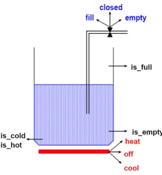
Figure 2:T,lcontrolled liquid
2.2 Abstraction and Formalisms
Abstract models of system behaviour can be described at different levels of abstraction or detail as well as by means of different formalisms. The particular formalism and level of abstraction depends on the background and goals of the modeller as much as on the system modelled. As an example, a temperature and level controlled liquid in a pot is considered. This is a simplified version of the system described in [BZF98], where structural change is the main issue. On the one hand, the liquid can be heated or cooled. On the other hand, liquid can be added or removed. In this simple example phase changes are not considered. The system behaviour is completely described by the following (hybrid) Ordinary Differential Equation (ODE) model:
dT
dt =
1 l[
W
cρA−φT] dl
dt = φ if 0<l<Helse 0
is low = (l<llow)
is high = (l>lhigh)
is cold = (T <Tcold)
is hot = (T >Thot)
The inputs are the filling (or emptying if negative) flow rateφ, and the rateW at which heat is
level
temperature
cold T_in_between hot
full
l_in_between
empty (cold,empty)
empty fill
empty fill
cool
heat
cool
heat (hot,full)
(hot,empty) (cold,full)
(cold,l_ib) (T_ib,l_ib) (hot,l_ib) (T_ib,full)
(T_ib,empty)
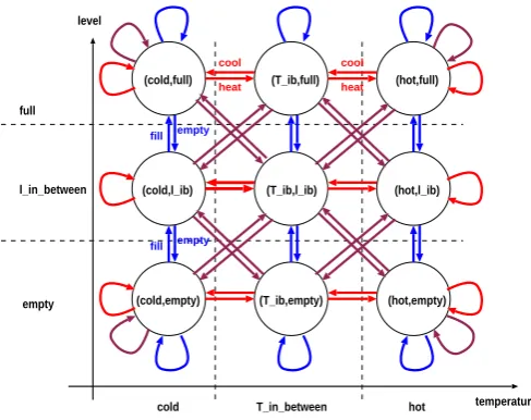
Figure 3: FSA formalism
dynamics of the system as depicted in Figure3is most appropriate.
Though at a much higher level of abstraction, this model is still able to capture the essence of the system’s behaviour. In particular, there is abehaviour morphism between both models: model discretization (from ODE to FSA) followed by simulation must yields the same result as simulation of the ODE followed by discretization.
2.3 Systems Theory
In general systems theory [Wym67], a causal (output is the consequence of input), deterministic (input will lead to unique output) system modelSY Sis defined. It is a template for a plethora of different formalims such as Ordinary Differential Equations, Finite State Automata, Difference Equations,etc.Its general form is
SY S≡ hT,X,Ω,Q,δ,Y,λi
T time base
X input set
Ω={ω :T →X} input segment set
Q state set
δ:Ω×Q→Q transition function
Y output set
λ:Q→Y (orQ×X→Y) output function
∀ω,ω0∈Ω,δ(ω•ω0,qi) =δ(ω0,δ(ω,qi)).
The time baseT is the formalisation of the independent variable time. Different ordering rela-tions (partial/total) can be used overT. Common time bases (with appropriate<and+) are
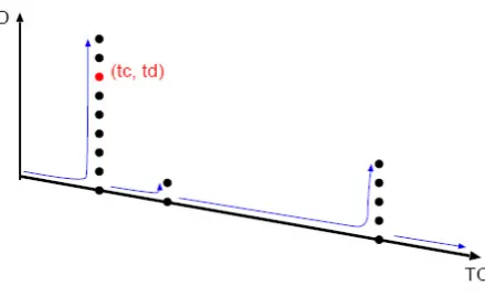
Figure 4: Time base for hybrid system models
• T =R. Models with this time base are calledcontinuous-timemodels. Note howdiscrete
event modelshaveRas a time base. However, only at a finite number of time-instants in a
bounded time-interval, an event different from the non-eventφoccurs.
• T=N(or isomorphic). Models with this time base are calleddiscrete-timemodels. Some
formalisms such as Finite State Automata (FSA) do not have an explicit notion of time (unlike their extension, timed automata). Hence, they are often called untimedmodels. There is however a notion of progression (from one state to another). According to our general definition, the index of progression, a natural number, is time.
Inhybridsystem models which combine aspects of continuous and discrete models [MB02], a
system evolves continuously over time (R) until a certain condition is met. Then,instantaneously
(the continuous time does not progress), the system may go through a number of discrete states (the index of progression is discrete) before continuing its continuous behaviour. To uniquely describe progression (of generalized time) in this case, a tuple (tc,td) depicted in Figure 4 is needed. Even when a series of discrete transitions keeps returning to thesamestate, the discrete indextcallows one to distinguish between them. The time base used is
T ={(tc,td)|tc∈R,td∈ {1, . . . ,N(tc)}}.
Here,N(tc) (≥1) describes the number of discrete transitions the system goes through at con-tinuous timetc. Obviously, only a partial ordering will be defined overT which consists of first testing the relationship between thetccomponents, and subsequently (if equal), that between the
tdcomponents.
In case of Partial Differential Equations (PDEs), the time base remainsR. The other
indepen-dent variables(often space in the form of some coordinate system) should be seen as infinitely
many state-variablelabelsorgeneralized coordinates.
The input setXdescribes all possible allowed input values (possibly a product set). An input segmentωrepresents input during a time-interval. The history of system behaviour is condensed
into astate(from a state setQ). The dynamics is described in a transition functionδwhich takes
T
T
T
T continuous
piecewise continuous
piecewise constant
discrete event V
V
V
V
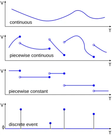
Figure 5: Segment types
the current input too). State and transition function must obey the composition or semigroup property. This property, whereby a transition over a time interval[ti,tf]can always be split into a composition of transitions over arbitrary sub-intervals, is the basis of all model simulators.
Figure5 shows some common segment types: continuous, piecewise continuous, piecewise constant and discrete event.
Note how for discrete event systems, inputs and output segments areevent segments
ω:ht1,t2i →A∪ {φ},
withφ the non-event. For such systems, the internal state behaviour is piecewise constant (the
internal state only changes at event times).
A host of formalisms are currently in use. In particular, through time-scale or parameter abstraction, reality is often represented by means of discrete-event models. In these models, time evolves continuously (T =R), but the state of the system only changes at a finite number
T:Continuous T:Discrete T:{NOW}
Q:Continuous DAE Difference Equations Algebraic Equations Q:Discrete Discrete event Finite State Automata Integer Equations
Naive Physics Petri Nets
Table 1: I/O system model classification
2.4 System classification
Formalisms can be classified based on the general system model structure (in particular, the type of time base T and state set Q) as shown in Table 1. More specific classifications are based on thestructureof formalisms. For continuous models, further classification according to physical domains such as mechanical, electrical, and hydraulical, is meaningful. The variety of classifications leads to the insight that ultimately, one should picture a vast formalism-space and classify that space according to various criteria. Different criteria will lead to different equivalence classes. Note how several exisiting modelling languages and tools may implement a single formalism.
3
Complex systems
3.1 Multi-component specifications
A common means to tackle complexity is to decompose a problemtop-downinto smaller sub-problems. Conversely, complex solutions may be builtbottom-upby combining primitive sub-problem solution building blocks. Both approaches are instances ofcompositional modelling: the composition ofinteracting componentmodels to build new models. In case the components
onlyinteract via their interfaces, and do not influence each other’s internal working in any other way (model information is completelyencapsulatedin object-oriented terminology, the compo-sitional modelling approach is calledmodular. If inter-components access is not restricted to take place via interfaces or ports only, the approach is callednon-modular.
3.2 Multi-formalism modelling
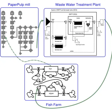
Complex systems are characterized, not only by a large number of components, but also by the diversity of the components. For the analysis and design of such complex systems, it is no longer sufficient to study the diverse components in isolation, using the specific formalisms these components were modelled in. Rather, it is necessary to answer questions about properties (most notably behaviour) of the whole system. To focus the attention, Figure6gives an example of a complex system.
The complexity lies in the diversity of the different components, both in abstraction level and in formalism used:
Figure 6: Complex system example
system is modelled as a process interaction discrete-event scheduling system.
• A Waste Water Treatment Plant (WWTP) takes the polluted effluent from the mill and purifies it. Some solid waste is taken to a landfill whereas the partially purified water flows into a lake. This system is modelled using Differential Algebraic Equations (DAEs) describing the biochemical reactions in the WWTP.
• A Fish Farm grows fish in the lake. Fish feed on algae which are highly sensitive to pol-luted water. The water is also used for a tree plantation which supplies the paper mill. This system is modelled using the System Dynamics formalism. The dotted feedback arrow from the fish farm to the paper mill indicates the possible disastrous impact of poisoned fish on the productivity of workers in the mill.
• the number of interacting, coupled, concurrent components. Complex behaviour is often a consequence of a large number of feedback loops.
• the variety of components such as software/hardware, continuous/discrete.
• the variety of views, at different levels of abstraction.
A model of a system such as the one described above may be valid (within a particular ex-perimental context) at a certain level of abstraction. This level of abstraction, which may be different for each of the components, is determined by the available knowledge, the questions to be answered about the system’s behaviour, the required accuracy of answersetc.Orthogonal to the choice of model abstraction level is the selection of a suitableformalismin which the model is described. The choice of formalism is related to the abstraction level, the amount of data that can be obtained to calibrate the model, the availability of solvers/simulators for that formalism as well as to the kind of questions which need to be answered.
Milner, in his Turing Award lecture [Mil93] rejects the idea that there can be a unique con-ceptual model, or one preferred formalism, for all aspects of something as large as concurrent systems modelling. Rather, many different levels of explanation, different theories, languages are needed. We believe this view is amplified when arbitrarily complex systems are studied.
As an introduction to the semantics of multi-formalism models we present the Formalism Transformation Graph (FTG) in Figure7.
The different formalisms are shown as nodes in the graph. The horizontal line at the bottom denotes the level at which trajectories can be described. The vertical dashed line demarcates con-tinous model formalisms (on the left) from discrete model formalisms (on the right). The FTG shows a plethora of formalisms, indicating that in general, many classifications are possible. It suffices to annotate the nodes in the FTG with attributes (possibly derived from the formalism structure) and determine equivalence classes based on those attributes. The arrows denote a ho-momorphic relationship “can be mapped onto”, implemented as a symbolic property-preserving transformation between formalisms. The vertical, dotted arrows denote the existence of asolver
orsimulation kernelwhich is capable of simulating a model, thus generating a trajectory. A
DEVS
Process Interaction Discrete Event
state trajectory data (observation frame) Petri Nets Statecharts
scheduling-hybrid-DAE
Bond Graph a-causal
Bond Graph causal DAE non-causal set
DAE causal set PDE
Transfer Function
Difference Equations
System Dynamics KTG
Cellular Automata
Event Scheduling Discrete Event
3 Phase Approach Discrete Event
DAE causal sequence (sorted)
DEVS&DESS
Activity Scanning Discrete Event
Timed Automata
Causal Block Diagram
Figure 7: The Formalism Transformation Graph (FTG)
Note that in theco-simulation approach, each of the sub-models in a coupled model is sim-ulated with a formalism-specific simulator. Interaction due to coupling is resolved at the trajec-tory level. Compared to transformation to a common formalim before simulation, this approach, though appealing from a software engineering point of view (it’s object-oriented) discards a lot of useful information. Questions canonlybe answered at the trajectory level. Furthermore, there are obvious speed and numerical accuracy problems for continuous formalisms [FY97]. The approach is meaningful only for discrete-event formalisms. In this realm, it is the basis of the DoD High Level Architecture (HLA) for simulator interoperability.
4
Conclusions
Bibliography
[Bal88] O. Balci. The implementation of four conceptual frameworks for simulation model-ing in high-level languages. In Abrams et al. (eds.),Proceedings of the 1988 Winter
Simulation Conference. Pp. 287–295. Society for Computer Simulation International
(SCS), 1988.
[Bal97] O. Balci. Principles of Simulation Model Validation, Verification, and Testing.
Trans-actions of the Society for Computer Simulation International14(1):3–12, March 1997.
Special Issue: Principles of Simulation.
[BZF98] F. J. Barros, B. P. Zeigler, P. A. Fishwick. Multimodels and Dynamic Structure Mod-els: an Integration of DSDE/DEVS and OOPM. In Medeiros et al. (eds.),Proceedings
of the 1998 Winter Simulation Conference. Pp. 413–419. Society for Computer
Sim-ulation International (SCS), 1998.
[Cel91] F. E. Cellier.Continuous System Modeling. Springer-Verlag, New York, 1991.
[CS92] B. A. Cota, R. G. Sargent. A Modification of the Process Interaction World View.
ACM Transactions on Modeling and Computer Simulation2(2):109–129, April 1992.
[FY97] L. Foster, K. Yelmgren. Accuracy in DoD High Level Architecture Federations. In Obaidat and Illgen (eds.),Summer Computer Simulation Conference (SCSC’97). Pp. 451–460. Society for Computer Simulation International (SCS), July 1997. Ar-lington, Virginia.
[Mag85] B. Magee.Popper. Fontana Press (An Imprint of HarperCollins Publishers), London, 1985.
[MB02] P. J. Mosterman, G. Biswas. A Modeling and Simulation Methodology for Hybrid Dynamic Physical Systems.Transactions of the Society for Computer Simulation
In-ternational, 2002.
[Mil93] R. Milner. Elements of Interaction. 36(1):70–89, January 1993. Turing Award Lecture.
[Wym67] A. W. Wymore.A Mathematical Theory of Systems Engineering – the Elements. Wiley Series on Systems Engineering and Analysis. Wiley, 1967.
[Zei84] B. P. Zeigler. Multifacetted Modelling and Discrete Event Simulation. Academic Press, London, 1984.
[ZPK00] B. P. Zeigler, H. Praehofer, T. G. Kim. Theory of Modelling and Simulation:
Inte-grating Discrete Event and Continuous Complex Dynamic Systems. Academic Press,