Volume 6: Graph Transformation and Visual Modeling Techniques 2007

(1)

Electronic Communications of the EASST

Volume 6 (2007)

Proceedings of the

Sixth International Workshop on

Graph Transformation and Visual Modeling Techniques

(GT-VMT 2007)

Bisimulation Verification for the DPO Approach with Borrowed

Contexts

Guilherme Rangel, Barbara K¨onig and Hartmut Ehrig

14 pages

Guest Editors: Karsten Ehrig, Holger Giese

Managing Editors: Tiziana Margaria, Julia Padberg, Gabriele Taentzer

(2)

Bisimulation Verification for the DPO Approach with Borrowed

Contexts

Guilherme Rangel1, Barbara K¨onig2and Hartmut Ehrig3

1_{[email protected]} 3_{[email protected],}

Institut f¨ur Softwaretechnik und Theoretische Informatik Technische Universit¨at Berlin, Germany

2_{barbara [email protected]}

Institut f¨ur Informatik und Angewandte Kognitionswissenschaft, Universit¨at Duisburg-Essen, Germany

Abstract:

Bisimilarity is the most widespread notion of behavioral equivalence and hence al-gorithms for bisimulation checking are of fundamental importance for verifying that two systems are behaviorally equivalent (seen from the perspective of the environ-ment). We investigate this problem in the context of behavioral equivalences of graphs and graph transformation systems, where the extension of the DPO approach to borrowed contexts provides us with a formal basis for reasoning about bisimilarity of graphs. In this paper we extend Hirschkoff’s on-the-fly algorithm for bisimula-tion checking, enabling it to verify whether two graphs are bisimilar with respect to a given set of productions. We then apply this framework to refactoring problems and verify instances of a model transformation which describes the minimization of deterministic finite automata.

Keywords:Bisimulation, Graph Transformation, Refactoring, Automata

1 Introduction

Model transformation [MV05] concerns the automatic generation of models from other models according to a transformation definition, which describes how a model in the source language can be transformed into a model in the target language. Such transformations can take place between different models or, more specifically, inside one single model (refactoring). Software refactoring is a modern software development activity to cope with the internal modification of source code to improve system quality, without changing the observable behavior.

(3)

found in [EE06, EW06, VVE+_{06]. A crucial question that must be asked is whether a given} refactoring (or model transformation) is behavior-preserving, which means that transforming one model into another model does not change the original external behavior. In practice, the proof of behavior-preserving transformations is not an easy task and therefore one normally relies on test suite executions and informal arguments in order to improve confidence that the behavior is preserved. In a recent paper Narayanan and Karsai [NK06] proposed a method for checking bisimilarity in model transformations using GTS which is similar to ours. The new contribution of our paper is to present an efficient bisimulation checking algorithm, which works on the fly for infinite state spaces, and to develop the theory in the very general framework of borrowed contexts [EK04].

In this paper we give a formal treatment of the question of behavior-preserving refactoring. We define model refactoring by graph transformation rules in the Double Pushout Approach (DPO) [CMR+_{97], which is one of the standards for GTS. Our goal is to show that instances} of one model are bisimilar to their refactored counterparts, which implies behavior preservation. We employ the extension of DPO to borrowed contexts [EK04], which provides the means to reason about bisimilarity. We also extend Hirschkoff’s [Hir01] on-the-fly bisimulation checking algorithm to deal with our setting. A case study of refactoring is presented in terms of minimiza-tion of deterministic finite automata (DFA), where we can test if a given DFA is bisimilar to its minimal refactored version. Since the procedure to check bisimilarity by hand is quite tedious we have implemented a tool in Objective Caml [OCa] to support this activity.

2 Graphs with Interfaces and Borrowed Contexts

In this section we recall the DPO approach to graph rewriting and its extension with borrowed contexts.

Definition 1 (Graph and graph morphism) Agraph G= (V,E,s,t,l_v,l_e) consists of a set V of nodes, a setE of edges, two functionss,t:E →V (source and target) and two labeling functions for nodes and edgeslv:V →ΩV,le: E→ΩE, whereΩV andΩE are node and edge

labels. Agraph morphism f:G₁→G₂is a pair of functions f= (f_E:E₁→E₂, f_V:V₁→V₂), which is compatible with source, target and labeling functions ofG1andG2, i.e., fV◦s1=s2◦fE,

fV◦t1=t2◦fE,le2◦fE =le1 andlv2◦fV =lv1.

In the standard DPO approach, graph productions rewrite graphs with no interaction with any other entity than the graph itself and the production. In the DPO with borrowed contexts [EK04] graphs have interfaces and may borrow missing parts of left-hand sides from the environment via the interface. This leads to open systems which take into account interaction with the outside world.

Definition 2(Graphs with interfaces and graph contexts) Agraph G with interface Jis a morphismJ →Gand a context consists of two morphismsJ →E ←J. Theembedding1 _{of a} graph with interfaceJ→Ginto a contextJ→E←J is a graph with interfaceJ→Gwhich is

(4)

obtained by constructingGas the pushout ofJ→GandJ→E. J //

²

² PO

E

²

J

o

¡

G //G

Definition 3(Rewriting with borrowed contexts) Given a graph with interfaceJ→Gand a productionp:L←I→R, we say thatJ→Greduces toK→Hwith transition label2_J_→_F_←_K if there are graphsD,G+_,_C_{and additional morphisms such that the diagram below commutes} and the squares are either pushouts (PO) or pullbacks (PB) with injective morphisms. In this case arewriting step with borrowed context(BC for short) is feasible: (J→G)−−−−−→J→F←K (K→H).

D_²_² // //

²

² PO

L_²_²

²

² PO

I

o

o //

²

² PO

R_²_²

²

G // //

PO

G+

PB

C

o

o //_H

J

O

/

/ //_F

O

K

o

O

O >>

Consider the diagram above. The upper left-hand square merges L and the graph Gto be rewritten according to a partial matchG←D→L. The resulting graphG+ _{contains a total} match ofLand can be rewritten as in the standard DPO approach, producing the two remaining squares in the upper row. The pushout in the lower row gives us the borrowed (or minimal) contextF, along with a morphismJ→F indicating howF should be pasted toG. Finally, we need an interface for the resulting graphH, which can be obtained by “intersecting” the borrowed contextFand the graphCvia a pullback. Note that the two pushout complements that are needed inDefinition 3, namelyCandF, may not exist. In this case, the rewriting step is not feasible. Let us also remark that the arrows depicted as→in the diagram above can also be non-injective (see [SS05]).

Note that our notion of labels exactly coincides with labels derived by relative pushouts [LM00,SS05].

3 Bisimilarity

Here we show how to use transition labels in order to check bisimilarity between two graphs with interfaces. A bisimulation is an equivalence relation between states of transition systems, associating states which can simulate each other.

Definition 4(Bisimulation and Bisimilarity) LetPbe a set of productions andRa symmet-ric relation containing pairs of graphs with interfaces(J→G,J→G0). The relationRis called a bisimulationif, whenever we have(J→G)R(J→G0₎_{and a transition}₍_J_→_G₎_{−−−−−→}J→F←K ₍_K_→

H), then there exists a graph with interfaceK→H0_{and a transition}₍_J_→_G0₎_{−−−−−→}J→F←K ₍_K_→_H0₎

(5)

such that(K→H)R(K→H0₎_.

We write (J →G) ∼(J→G0)whenever there exists a bisimulation R that relates the two graphs with interface. The relation∼is calledbisimilarity.

In the graph setting not all labels that can be derived from a graph and a set of productions are relevant for the bisimulation. We will distinguish two kinds of transition labels.

Definition 5 Let (J → G) −−−−−→J→F←K (K →H) be a transition of (J → G). We say that the transition isindependentwhenever we can add two morphismsD→JandD→Ito the diagram inDefinition 3such that the diagram below commutes, i.e.,D→I→L=D→LandD→J→ G=D→G. We write(J→G)−−−−−→J→F←K _d(K→H)if the transition is not independent and we call itdependent.

D //

²

º

'

L

²

I

o

o //

²

R

²

G //G+ oo _C // _H

J

O

/

/ _F

O

K

o

O

O >>

An independent label has a borrowed contextF that provides the entire left-hand sideLfor Gand henceGdoes not contribute to the rewriting. (A trivial example is a label derived with D=/0.) The figure above on the right schematically depicts this situation where the partial match occurs only in the overlap of the interfacesJandIleading to an independent label.

The bisimulation game for graphs mainly takes dependent labels into account. That is, if we modifyDefinition 4in such a way that only dependent transitions(J→G)−−−−−→J→F←K _d(K→ H) have to be simulated (either by a dependent or independent transition), then the resulting bisimilarity∼is unchanged (see [EK04]).

One of the main advantages of the borrowed contexts technique is that the derived bisimilarity is automatically a congruence, which means that whenever one graph with interface is bisimilar to another, one can exchange them in a larger graph without effect on the observable behavior. This is very useful for model refactoring since we can replace one part of the model by another bisimilar one.

Theorem 1(Bisimilarity is a Congruence[EK04]) The bisimilarity relation∼is a congru-ence, i.e., it is preserved by contextualization as given inDefinition 2.

(6)

is given byFcontext_{, which embeds all pairs into the same contexts (as in} _{Definition 2), for all}

pairs and all compatible contexts.

The search of dependent labels among several partial matches might lead to cases where the pushout complementF orC(seeDefinition 3) does not exist and so the borrowed context step is not feasible. In [BGK06] a technique, based on initial pushouts, is defined to check if a partial match allows the existence ofFandC.

Proposition 1 [BGK06] Let p: L←I →R be a production and f: D→L a monomorphism such that the diagram below on the left is the initial pushout of f . The pushout complement F

ofDefinition 3exists if and only if there is a monomorphism D→G and a morphism JD→J

such that the diagram on the right commutes. JD //

g

²

² IPO

FD

²

D _f //L

JD g //

²

² =

D

²

J //G

Symmetrically one can check that the pushout complement C exists by taking the initial pushout overD→G.

4 Partial Match Finding

Here we propose an algorithm that takes as input a graph with interfaceJ→Gand a setP of productions of the formp:L←I→Rto find all possible partial matchesG←D→Lthat will lead to dependent labels. We first need to introduce partial morphisms.

Definition 6(Partial graph morphism) LetG= (V,E,s,t,lv,le)be a graph as inDefinition 1.

Asubgraph SofG, writtenS⊆G, is a graph withVS_⊆_VG_, _ES_⊆_EG_,_sS₌_sG_|

ES,tS=tG|_ES, lS

v =lvG|VS and l_eS=l_eG|_ES. A partial graph morphism f: G*G0 is a total graph morphism f:dom(f)→G0from a subgraphdom(f)⊆GtoG0.

GivenL(the left-hand side of a production) andG, we try to find partial matches which lead to a feasible BC step with a dependent label. We describe a procedure in 5 steps for one single productionp, but it must be carried out for all productions ofP. Step1determines a subgraph Lclean _of_L_{, which is the largest subgraph of}_L_{containing only node and edge labels that also}

occur inG. The graphGclean_{is defined analogously (with the roles of}_L_and_G_{exchanged). Step}

2creates all possible subgraphsLsub

i (i∈N) ofLclean. Step3finds all injective partial matches

pm_j: Lsub

i *Gclean (j∈N). Step 4 splits each partial matchpmj as a span of total injective

morphismsL←Lclean ←Dj →Gclean→G. Step5 storesL←Dj →Gas a partial match to

derive a label ifL←Dj→Gsatisfies the conditions ofProposition 1(for the existence ofFand

(7)

5 Matching Labels and Existence of Derivable Labels

The bisimulation game for graphs demands the comparison of labels. More specifically, two labelsµi=Ji→Fi←Ki(i=1,2) are called isomorphic (µ1∼=µ2) if they are isomorphic cospans.

Remember that a dependent label can be answered by either a dependent or independent label. Since the algorithm in the previous section derives only dependent labels, we propose a way to check whether a dependent label for one graph is also derivable for the other graph. This if more efficient than deriving all independent labels for the other graph, which could be a lot, and checking whether they match.

Definition 7(Derivable Label) Given a graphJ→G, a labelJ0→F0 ←K0 and a setP of productions, we say thatJ0_→_F0_←_K0_is_derivable_from_J_→_G_and_P_{if it yields a feasible BC}

step, as inDefinition 3.

D //

²

² PO(PB)

L

mi

1

²

² PO

I

o

o //

PO

²

R

²

G _m2 //G+ oo _C //_H

J _∼ //

?

Ä Ä Ä Ä Ä Ä Ä

Ä ((

J0 //

PO

F0

PB

O

K0

o

O

O >>

This can be checked as follows: if there exists an isomorphism J →∼ J0 we obtain J →F0 as the compositionJ →∼ J0 _→_F0 _{and in addition}_G_→_G+ _←_F0 _{as a pushout of}_G_←_J_→_F0_.

For all productions P we find all possible total matches mi

1: L→G+ (i∈N). For each mi1

and m2: G→G+, if mi1 and m2 are jointly surjective (i.e., m1i,V(LV)∪m2,V(GV) =G+V and

mi

1,E(LE)∪m2,E(GE) =G+E) we can takeG←D→Las a pullback ofG→G+←Land thus

obtain a pushout. We compute the pushout complementG+_←_C_←_I _of_G+ _←_L_←_I _{and the} pushoutC→H←RofC←I→R. We then check if there exists a morphismK0→Csuch that the rightmost square in the second row is a pullback and add the induced morphismK0_→_H_{. If}

there exists a total matchmi

1:L→G+, which allows us to complete this diagram, we say that the

labelJ0→F0←K0 is derivable fromJ→GandP. Note that this is easier than partial match finding since we are only looking for total matches.

6 Algorithm for Bisimulation “On the Fly”

Classical methods for bisimulation checking (e.g., see [PT87]) take as input the full state spaces which are derived from the initial processes to be compared. Their drawback is that the whole state space must first be computed and stored. Fernandez and Mounier defined in [FM91] a method for building the state space on the fly and checking bisimilarity based on depth-first search (DFS). Hirschkoff [Hir01] extended their work to not only allow breadth-first search (BFS), but also to deal with bisimulation up-to.

(8)

evolve along the same labelµ, i.e.,(P,Q)→µ (P0_,_Q0₎_{. The algorithm initially checks whether}_P

andQare immediately bisimilar (none of them has further labels leading to successor states) or non-bisimilar (one makes a step which the other is not able to mimic). IfPandQare not found immediately (non-)bisimilar, their state space product is expanded by adding their successors reached by a common label and so the bisimilarity of(P,Q)can be only known after the recursive analysis of all successors in the state space product. With this basic technique the LTSs in question must be finite. But in some cases the algorithm is able to perform finite proofs for states whose state space product is infinite using up-to techniques in order to handle infinite bisimulations as finite bisimulations up-to. Hirschkoff proved that the breadth-first version of the algorithm is computationally complete with respect to a given up-to techniqueF, which means that the algorithm can check the bisimilarity of two states if and only if a finite bisimulation up toF relating the two states to be checked exists. Hirschkoff used his algorithm to check bisimilarity of polyadicπ-calculus [Mil93] processes.

We extend Hirschkoff’s algorithm to check bisimilarity between graphs with interfaces with respect to a given set of graph productions. We also did minor efficiency improvements and added extra details to the algorithm, trying to make clear aspects that were not easy to understand in the original version.

Remember that in order to calculate all dependent labels which originate from a given graph with interface and a setPof productions we employ the algorithm defined inSection 4to find partial matches between the left-hand side of the rules ofP and the graph with interface. For every partial match we then useDefinition 3to complete the whole borrowed context diagram, which gives us the dependent label and the resulting graph with interface. The matching of labels is specified inDefinition 7.

In the setting of graphs, the bisimulation checking algorithm explores the state space prod-uct (defined below) of two graphs to be compared. We use here some shortcuts: graphs with interfacesJ→Gare represented asPandQ, and labelsJ→F←Kasµ.

Definition 8(State Space Product) The state space productof two graphsP0 andQ0 is the

transition system generated from the initial state(P0,Q0)using the following inference rules:

dep1 : P

µ

−→dP0 _Q_−→µ0 _Q0

(P,Q)−→µ (P0_,Q0₎ dep2 :

P−→µ P0 _Q_−→dµ0 _Q0 (P,Q)−→µ (P0_,Q0₎ µ

∼

=µ0

The successors of(P,Q)are all(P0_,_Q0₎_{such that}_P0_and_Q0_{respectively correspond to}

evolu-tions ofPandQalong an isomorphic labelµ. The rulesdep1anddep2cover the situation when one dependent label (indicated with→_dabove) is answered (i.e. matched) by either a dependent or independent isomorphic label. If one graph can not answer, we say that the pair fails to evolve, i.e., we can infer immediately thatPandQare not bisimilar.

Definition 9(Failure) Given two graphsP andQwe say that the pair(P,Q) fails to evolve whenever it holds:

(P −→µ _d P0_∧_@_Q0_:_Q _−→µ0 _Q0 _s.t. _µ ∼₌_µ0₎_∨₍_Q ₋_→µ

d Q0∧@P0:P

µ0

−→ P0 _s.t. _µ ∼₌_µ0₎_.

(9)

three setsV,W andR, containing pairs of graphs that are respectively supposed to be bisimilar, known to be non-bisimilar and known to be bisimilar. By accessingSas stack (resp. queue) the algorithm performs a depth-first (resp. breadth-first) search on the state space product.

The main procedure isbisimulation check, which calls:succeeds,failsandpropagate. The procedurebisimulation checkfirst checks withsucceedswhether(P,Q)is immediately bisimi-lar (e.g. none of them is able to derive any further (dependent) label). If(P,Q)is not immediately bisimilar,failschecks if the pair fails to evolve or if it is already known as non-bisimilar (i.e., it is inW). If it fails we insert it intoW and usepropagateto update the information about the state space product inTablewith this new result, which can possibly lead to the discovery of new (non-)bisimilar graphs. When we find that a new pair evolves to other pairs, we assume that it is bisimilar (insert it intoV) and only after the analysis of all its successors (where the notion of successor is specified inDefinition 8) we are able to decide whether the pair is really bisimilar (as we assumed) or not. If by processingSwe find a pair that is inV (supposed to be bisimilar) we move it toRand updateTableusingpropagate. When all pairs have already been analyzed (S=/0) the algorithm can determine the bisimilarity of(P,Q).

a

(3,5) (1,4) (3,6)

S

b (3,6)

(2,5) (3,5)

fails (2,6)

fails 2 3

a a

1

b _{5 6}

a a

4

b

(1,4)

a a a

Table

(P,Q) successors m fails

(1,4) (2•,5)(2•,6)(3◦,5)(3◦,6) £¤ £ ¤2 3 5 6 false

(3,5) true

(3,6) (3◦,6) ¤¤3 6 false

Above, one can see two small transition systems, their respective state space product, the states under investigation inSand their current information inTable. The states 1–6 represent graphs anda,bare labels. Consider the pair(1,4)inTable. The entrysuccessorsshows the successors of(1,4)in the state space product together with a boolean valuetrue(•) orfalse(◦), indicating which pairs of successors have already been analyzed. The entrym lists the successor states (e.g. 3 and 6 withfalse[¤], 2 and 5 withtrue[£]), indicating which state has found a bisimilar partner. Whenever a pair of successors has been analyzed, if it turns out to be bisimilar both m-fields of the pair are set totrue(£). Successors(2,5)and(2,6)have been explored and only

(2,5)is bisimilar. If all successors of(P,Q) have been analyzed (all are set to•) and all fields ofmare set to true (£) then (P,Q) is bisimilar. If there is in mat least one graph with false (¤) then(P,Q) is not bisimilar. The entryfails indicates if a pair fails to evolve (according to Definition 9). A non-bisimilar pair has always at least one successor leading to a failure, but it is worth observing that a bisimilar pair might also have successors leading to a failure. In the example even though(2,6)and(3,5)fail, it is clear that(1,4)is bisimilar.

(10)

bisimulation check(P,Q):=

W:=/0;

(∗)R:=/0;V:=/0;

insert(P,Q)intoSandTable;status:=true; while S6=/0do

take(P0,Q0)fromS;

if succeeds((P0,Q0))

theninsert(P0,Q0)intoR; propagate((P0,Q0),true); else if fails((P0,Q0))

theninsert(P0,Q0)intoW; propagate((P0,Q0),false);

else if (P0,Q0)∈V

thenmove(P0,Q0)fromVtoR; propagate((P0,Q0),true);

else if (P0,Q0)∈R

then propagate((P0,Q0),true); else{pair(P0,Q0)is new}

insert(P0,Q0)intoV; {(P0,Q0)→µ successor(P0,Q0)} insert successors of(P0,Q0)intoS; for eachsuccessor(P0,Q0)do

ifsuccessor(P0,Q0)∈/Table

∧successor(P0,Q0)∈/W∪R∪V

theninsert it intoTable; end for

end while if(P,Q)∈/R

thenreturnfalse

else ifstatusthenreturntrueelseloop back to(∗)

succeeds(P,Q):=Table(P,Q).successors=/0

∧Table(P,Q).fails=false

fails(P,Q):= if(P,Q)∈Table

thenTable(P,Q).fails∨(P,Q)∈W

else(P,Q)∈W

propagate((P,Q),success):=

if(P,Q)∈R∧success=false

thenstatus:=false; if(P,Q)∈Table

∧Table(P,Q).successors is complete3 thenremove(P,Q)fromTable;

for each(Pf,Qf)∈Tablewith(Pf,Qf)→µ (P,Q)do

Table(Pf,Qf).successors(P,Q):=true; ifsuccess

thenTable(Pf,Qf).m(P):=true;

Table(Pf,Qf).m(Q):=true; ifTable(Pf,Qf).successorsis complete

then

if∃j=false∈Table(Pf,Qf).m then

insert(Pf,Qf)intoW; propagate((Pf,Qf),false); else

if(Pf,Qf)∈V

thentake it fromVtoR; propagate((Pf,Qf),true); end for

The procedurepropagate is in charge of updating the information inTableconcerning the state space product analysis. Every time we rediscover a new pair we decide that it is bisimilar (i.e., it is moved toR). If during the exploration of the state space we find that this very pair is non-bisimilar we set the variablestatustofalse, which means that the result of the current run of the algorithm is not reliable. In this case we restart it retaining the information inW about states which are already known to be non-bisimilar.

The procedurepropagatekeeps inTableonly the pairs under analysis, removing the ones that have already been analyzed. Observe that when one pair is propagated, the predecessors of this pair should also be informed of the new results. When a pair is propagated withtrue orfalse the algorithm always sets this pair as analyzed (true[•]) in the list ofsuccessorsof each of its predecessors that are still under analysis (inTable). Only if the pair is propagated withtrueits respective graphs inmof its predecessors are set totrue(£). When the last successor of a given pair has been analyzed we can verify whether our initial hypothesis about its bisimilarity is still true. If the pair has at least one graph inmset asfalseit is non-bisimilar (our hypothesis was wrong) and we propagate this result. Otherwise we conclude that our hypothesis was correct and propagate this information.

If the algorithm has to handle bisimulation up-to we have only to replace inbisimulation check

(P0,Q0)∈V by (P0,Q0)∈F(V) and (P0,Q0)∈R by (P0,Q0)∈F(R), where F

de-scribes the up-to technique. For the refactoring proposed in this paper (seeSection 8) we use

(11)

the up-to context technique (Fcontext_{) [EK04] informally described in}_{Section 3.}

Our version of the bisimulation checking algorithm is very similar to Hirschkoff’s. Our main contribution to the algorithm is the full specification of howTableis used to store and process the state space product investigation. A small efficiency improvement can be seen in thefor each statement ofbisimulation check, where we added extra conditions in order to avoid reanalyzing pairs already investigated. Furthermore we checked that the algorithm also works in our setting of borrowed contexts, taking into account especially the issue of independent and dependent labels.

7 Tool Support for DPO with Borrowed Contexts

The derivation of labels and the bisimulation proof demand a great amount of time even for small examples and when done by hand they are particularly susceptible to errors. To overcome this we have implemented a tool in Objective Caml (OCaml), which is a functional language very appropriate for rapid prototyping. The tool uses directed labeled graphs and when we want to check the bisimilarity of two graphs, we specify a set of graph productions and also the graphs with interfaces to be checked. We have already implemented graphs with interfaces, graph productions, and procedures for label derivation and matching. OCaml is mainly textual, but for the sake of visualization, our graphs, rules and derived labels can be visualized with the package Graphviz [gra]. Our next goal is to implement the described algorithm for bisimulation checking.

8 Refactoring Deterministic Finite Automata

We will now come back to our original motivation: showing that refactoring preserves behav-ior. Let us first explain how the current theory of DPO with borrowed contexts could be used to prove that a refactoring process is behavior-preserving. Consider a modelM, whose operational semantics is given by a set OpSemM _{of graph productions and a refactoring for this model}_M

as a setRefactoringM of productions of the form L←I →R. If we can prove for each rule of RefactoringM that we have the bisimilarity (I →L)∼(I →R) with respect to OpSemM, this means that each rule does not change the behavior of the model under refactoring. Since bisim-ilarity is a congruence we can compose (I →L) and(I→R) with identical contexts and the respective compositions remain bisimilar. That is, for all instances ofM,RefactoringMpreserves the original behavior. This approach can be currently used only for refactoring rules without features such as negative application conditions and layers, which are often necessary to model refactorings.

(12)

is consumed by a DFA, this means that the string previously processed was accepted.

accept W

W

W W

0 ₁

1

0 FS

FS

0

DFA2

DFA1 Loop

Jump Accept

a a

a

a a

a

a 1

FS

0

0 1

a W

W

FS

FS FS

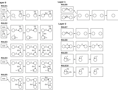
Below we define graph productions to minimize DFAs by eliminating equivalent states. The idea of the algorithm is to identify the distinguishable states, followed by the merging of equiv-alent states. Note that to the left of each rule we depict the negative application conditions. The algorithm is defined by several graph productions spread over three layers, where each layer ap-plies its rules as long as possible before the rules of the next layer can be used. In practical terms, the transformation begins with rules of layer 0. If no more rule of layer 0 is applicable, the rules of layer 1 come into play. The rules inlayer 0(seeFigure 1) examine the transitions labels for every two states and determine if they are distinguishable. The rule inlayer 1merges equivalent nodes, i.e., nodes without adistedge between them. Finally, the rules inlayer 2remove alldist edges and redundant transitions between two states.

Observe that the minimization algorithm demands rules spread over layers and negative ap-plication conditions and so we are not able to prove that all refactorings via these rules are behavior-preserving. For this reason our goal in this paper is to check that a given DFA and its minimal refactored version are bisimilar. Note that for DFAs borrowed context bisimilarity coincides with language equivalence. Furthermore in our setting bisimilarity on automata seen as transition systems corresponds to the bisimilarity that we obtain via the borrowed context technique.

(13)

FS dist FS 1 1 RHS FS FS a a a a dist a 1 a

FS FS FS

1 RHS FS RHS dist a a dist a a dist a a dist RHS a dist a a dist a a a dist dist RULE4 a dist a dist a dist a a dist a RHS RULE5 a a a a a a a a FS FS FS FS RULE3 RULE2 RULE1 Layer 0 Layer 2 Layer 1 dist dist RULE6 dist RULE7 RULE8 RULE9 RULE10

Figure 1: Productions for DFA minimization

9 Conclusions and Future Work

We have shown how to use the DPO approach with borrowed contexts to automatically check the bisimilarity of systems specified in terms of graphs. Furthermore we suggested as a case study for refactoring the minimization of DFAs.

Our plan is to extend this work in such a way that whenever we define a refactoring as graph productions we should also be able to prove that all instances prior to refactoring are bisimilar to their refactored counterparts. The first step to be made to accomplish such an objective is the extension of the current theory of DPO with BC to handle rules with negative application conditions and layers, which are often used in refactorings.

(14)

FS w w w w w w w w w w w w w w w

w w w

w w w w w w w w w w w 1 0 1 1 FS w 1 0 0 w w w w accept 0 0 1 FS FS 0 1 0 accept ₀ 1 1 w 0 FS 0 1 1 w

1 0 ₁

FS 0 0FS

1 1 w 0 FS 0 1 1 1 w 0 0 ₁ 0 FS

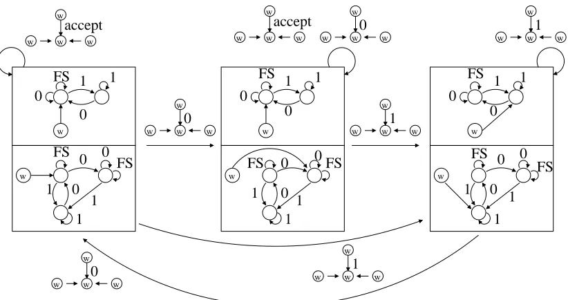
Figure 2: State space product for DFA1 and DFA2

Bibliography

[BGK06] F. Bonchi, F. Gadducci, B. K¨onig. Process Bisimulationviaa Graphical Encoding. In Corradini et al. (eds.), Proc. of ICGT’06. LNCS 4178, pp. 168–183. Springer, 2006.

[CMR+_97] _{A. Corradini, U. Montanari, F. Rossi, H. Ehrig, R. Heckel, M. Loewe. Algebraic} Approaches to Graph Transformation Part I: Basic Concepts and Double Pushout Approach. In Rozenberg (ed.), Handbook of Graph Grammars and Computing by Graph transformation, Volume 1: Foundations. Pp. 163–246. World Scientific, 1997.

[EE06] H. Ehrig, K. Ehrig. Overview of Formal Concepts for Model Transformations Based on Typed Attributed Graph Transformation. InProc. of GraMoT ’05. ENTCS 152, pp. 3–22. Elsevier Science, 2006.

[EK04] H. Ehrig, B. K¨onig. Deriving Bisimulation Congruences in the DPO Approach to Graph Rewriting. In Walukiewicz (ed.), Proc. of FoSSaCS ’04. LNCS 2987, pp. 151–166. Springer, 2004.

[EW06] K. Ehrig, J. Winkelmann. Model Transformation From VisualOCL to OCL Using Graph Transformation. InProc. of GraMoT ’05. ENTCS 152, pp. 23–37. 2006.

[FM91] J.-C. Fernandez, L. Mounier. On the Fly Verification of Behavioural Equivalences and Preorders. InProc. of CAV’91. LNCS 757, pp. 181–191. Springer-Verlag, 1991.

(15)

[Hir01] D. Hirschkoff. Bisimulation Verification Using the Up to Techniques.International Journal on Software Tools for Technology Transfer3(3):271–285, Aug. 2001.

[LM00] J. J. Leifer, R. Milner. Deriving Bisimulation Congruences for Reactive Systems. In Proc. of CONCUR ’00. Volume 1877, pp. 243–258. Springer-Verlag, London, UK, 2000.

[Mil93] R. Milner. The polyadicπ-Calculus: a tutorial. In Hamer et al. (eds.), Logic and Algebra of Specification. Springer-Verlag, Heidelberg, 1993.

[MT04] T. Mens, T. Tourwe. A Survey of Software Refactoring.IEEE Transactions on Soft-ware Engineering30(2):126–139, 2004.

[MV05] T. Mens, P. Van Gorp. A Taxonomy of Model Transformation. InProc. of GraMoT ’05. Volume 152, pp. 125–142. 2005.

[NK06] A. Narayanan, G. Karsai. Towards Verifying Model Transformations. In Bruni and Varr´o (eds.),Proc. of GT-VMT ’06. ENTCS, pp. 185–194. Vienna, 2006.

[OCa] Objective Caml.http://caml.inria.fr/ocaml/.

[PT87] R. Paige, R. E. Tarjan. Three Partition Refinement Algorithms.SIAM Journal on Computing16(6):973–989, 1987.

[San95] D. Sangiorgi. On the Proof Method for Bisimulation. In Wiedermann and H´ajek (eds.),Proc. of MFCS ’95. LNCS 969, pp. 479–488. Springer, 1995.

[SS05] V. Sassone, P. Soboci´nski. Reactive systems over cospans. In Proc. of LICS ’05. Pp. 311–320. IEEE, 2005.