International Journal Advances in Social Science and Humanities
Available online at: www.ijassh.com
RESEARCH ARTICLE
Persistence of Terms of Trade Shocks and Real Exchange Rate
Volatility in Nigeria
Ngwudiobu Ikenna M, Emecheta Chisom*, Aidi Olatunji H
Department of Economics, University of Nigeria, Nsukka.
Abstract
This study is undertaken to determine the duration of terms of trade shocks, estimate its impact on real exchange rate volatility and proffer policies that may help dampen its volatility. The study adopted the median unbiased estimation procedure to calculate the duration of terms of trade shocks in Nigeria. This procedure follows a first order autoregressive AR (1)/unit root model. Thereafter, the impact of terms of trade shocks on real exchange rate volatility was estimated using the distributed lag model based on an Error Correction Model (ECM). This study reveals that terms of trade shocks is not a very serious case in Nigeria due to its temporal effect, notwithstanding its positive impact on real exchange rate volatility. The study discovers that terms of trade shocks have an immediate high magnitude of impact in the current period than after one year in Nigeria. The study recommends that the non-oil exports be diversified to include a huge percentage of manufacturing products so as to add value to raw materials which hitherto constituted the major component of non-oil exports. Also, depreciating the real exchange rate a little will create a more conducive atmosphere for investors in the economy.
Keywords: Terms of Trade Shocks, Persistence, Real Exchange Rate Volatility, Median-Unbiased Estimation, Distributed Lag Model and Error Correction Model (ECM).
Introduction
Investors in any economy are uncertain whether to invest their hard earn money or not in a scenario of real exchange rate volatility. Ezema [1] noted that volatility in the real exchange rate is common with countries under high terms of trade shocks. The World Bank [2] report shows that for the period of 1961 to 2000, Nigeria is in the top five of world’s highest terms of trade shocks and real exchange rate volatility. The real exchange rate volatility affects the profitability of investments through price channels and through the cost of borrowing. Risk averse investors in different sectors of the economy will develop a lukewarm attitude towards investment until they are more certain about future profitability, while those who must have already invested might suspend the investment in favor of something more lucrative (perhaps saving their money in the bank) because the economic environment is less conducive to undertake such risk.
According to Mankiw [4] there is negative relationship between the real exchange rate and net exports. Depreciation in the real exchange rate shows that domestic goods are relatively cheaper than foreign goods. This makes net exports greater. The reverse is always the case when there is an appreciation in the real exchange rate. With
real exchange rate depreciation, there will be fewer incentives for imported goods. This stimulates domestic investment and also is quite capable to spur domestic output. The table below shows the average movements in the growth rates of real exchange rate (RER) and terms of trade (TOT) in Nigeria.
Table 1: Volatility and averages of real exchange rate and terms of trade
Eight year range RER Volatility Average growth rate
of RER (percent) Average growth rate of TOT (percent)
1982 – 1989 33.84 -9.4 6.2
1990 – 1997 36.46 19.9 -8.9
1998 – 2005 28.95 -4.9 -0.5
2006 – 2013 6.51 4.5 -4.7
Source: World Bank (2015) Database and Author’s Computation Based on 8-Year Standard Deviations of Growth Rate (Volatility) and Averages of variables [5].
The movement in the average growth rate of the variables as well as the volatility in the real exchange rate in the above table shows how the variables fluctuate over an eight year range. A positive growth rate in the real exchange rate shows an average appreciation in the real exchange rate, while a negative real exchange growth rate shows an average depreciation. On the other hand, a positive terms of trade growth rate shows an average favorable terms of trade, while a negative terms of trade growth rate shows an average unfavorable terms of trade. The table above shows that the terms of trade have been more favorable on the average of about 6.2percent within the 1982-1989 periods. This has, however, fluctuated within the unfavorable limit. The real exchange rate fluctuated from an average depreciation to an average appreciation and so on within the eight year range periods. By way of comparison, an average depreciation of the real exchange rate of 9.4percent accompanies an average favorable terms of trade growth rate of 6.2 percent for the 1982-1989 periods. However, for that of 1990-1997, there is an appreciation in the average growth rate of the real exchange rate of 19.9percent which is accompanied by an unfavorable average growth rate of the terms of trade of 8.9percent. There happens to be a mix up in signs for the period of 1998-2005, but comparing the magnitudes with the first year period (1982-1989) depicts the same interpretation. The last period (2006-2013) shows the same
interpretation with the second period (1990-1997). The table also shows a case of unfavorable terms of trade shock and real exchange rate volatility from historical data.
The World Bank [2] report shows that the reason behind Nigeria’s extreme terms of trade shocks is the very concentrated nature of her oil exports, relative to its well diversified non-oil imports and also oil price shocks. Iwayemi [6] observed that a decline in price of crude oil further deteriorated the terms of trade in Nigeria, thus leading to unfavorable terms of trade shock and this played key roles on the sharp decline in investment, which is quite capable to hamper growth. Ezema [1] stated that there is no country in the world that has not experienced terms of trade shocks at one time or the other. Thus, it is the policy thrust among the countries that make the difference. Cashin and Pattilo [7] noted that the duration of terms of trade shocks are important as it informs the appropriate policy response to take. Cashin and Pattillo further argued that based on the associated problems that comes with terms of trade shocks, nobody can assess a country’s economic policy without being acquainted with the uncertainty that surrounds the future movements in her terms of trade [7].
volatility of the economy. But going by the same logic, alternative policy choices could help reduce the level of real exchange rate volatility which of course will help stimulate growth. Apart from Naude [8] an Ethiopian study, the researchers are not aware of any country specific study that have tried investigating the duration/persistence of terms of trade shocks in Nigeria and beyond. It is the persistence of terms of trade shocks that will pave way for the envisaged alternative policy choices that will improve the state of the economy. Thus, to seek the validity of the policy choices to the terms of trade shocks, the following questions will be addressed. What is the duration of terms of trade shocks in Nigeria? What is the impact of terms of trade shocks on the volatility of real exchange rate in Nigeria?
The remainder of this paper will be outlined as follows. Section 2-literature review, will give a concise conceptual review, theories and empirical evidences. Section 3 will introduce the data and methodology sufficient enough to answer the research questions. Section 4 will present and analyse the empirical results and finally, section 5 will conclude the paper and provide the long awaited alternative policy actions to take.
Literature Review
The terms of trade is an economic variable that shows how a country’s exports pays for her imports. This is measured as the ratio of the export price index and import price index. Broda [9] noted that this variable fluctuates over time, most especially for developing countries because they have little or no leverage over the prices for their exports. Thus, terms of trade shocks according to Andrews and Rees [10], can be seen as an unanticipated fluctuation in the terms of trade. The real exchange rate according to Mankiw [4] can be seen as the relative price of the goods of two countries. This tells us the rate at which we can trade the goods of one country for the goods of another. This is measured as the product of nominal exchange rate and the ratio of price levels (the ratio of foreign price level to domestic price level). The real exchange rate is sometimes called the terms of trade if each country produced only one type of good, so that home and export sales will be the
same. However, Black [11] noted that as home sales typically include non-traded goods, and the composition of exports and home sales of exportables usually differs, the real exchange rate should not be confused with the terms of trade. Volatility in the real exchange rate also means an unanticipated fluctuation (appreciation and depreciation) in the real exchange rate.
In an attempt to express the understanding of how export and import value/price indices affect a country’s terms of trade, Broda and Tille [9] considered a simple example in which a country exports wheat and imports oil. An increase in the price of oil (imports) depicts a worsening terms of trade because the country will pay more for the goods it imports. On the other hand, an increase in the price of wheat (exports) boosts the country’s export earnings, thus improving its terms of trade. Also according to Obstfeld [12] a rise in the terms of trade increases a country’s welfare, while a decline in the terms of trade reduces it.
Baxter and Kouparitsas [13] however, pointed out some of the causes of the unanticipated volatility in terms of trade (terms of trade shocks) in twofold. First, terms of trade shocks are highly prevalent in developing countries as a result of their heavy reliance on commodity exports, where prices are more volatile, relative to those of manufactured goods in developed countries. Second, most developing countries are known traditionally to have a high degree of openness (this shows the extent to which a country is prone to external shocks) to foreign trade. This consequently paves way for sharp swings in their terms of trade which affects a large share of their economies. In addition, Broda [9] noted that developing countries are plagued by terms of trade shocks because they are mainly small open economies. This suggests that they cannot have influence on world’s relative supply and demand, thereby having little or no leverage over their export prices. This makes the terms of trade shocks of developing countries largely exogenous.
believes that a quick resolution of such unexpected problem is a bold step in addressing the distortions associated with terms of trade shocks. Cashin and Pattillo [7] opined that an inquiry into the difficult task associated with ascertaining if the terms of trade shocks are permanent or temporal is much more proactive to launch proper policy measures to address its issues. Ezema [1] noted that most researchers are of the opinion that adjusting to shocks on the terms of trade can be done through two conservative approaches. First is by saving during a favourable terms of trade shock and second, by avoiding irreversible commitments or commitments that are costly to reverse in a period of high uncertainty about the future.
According to Gavin [15], some economists are bent on taking such commitments for the purpose of a smooth path of consumption, known as permanent income hypothesis. They argue that if deteriorating terms of trade shock is perceived to be persistent, it leads to a permanent lower level of income. This suggests that it is safer for consumption to decline immediately to the new level of income. On the other hand, if the shock is perceived to be temporal, then it does make sense to borrow from abroad to cushion the short-run effects on domestic expenditure. Gavin however, noted that such temporal solution could be applied to the production sector. This is because it takes time to adjust in this sector, thus even permanent shock in the terms of trade should be financed by borrowing.
The studies of Harberger [16], Laursen and Metzler [17] proposed that positive terms of trade shock should cause an increment in real income, aggregate savings – due to a marginal propensity to consumption less than one – and, thus, an improvement to the current account. On the other hand, when terms of trade worsen, net exports and savings decline because a fall in the purchasing power of exports is a reduction in income and the marginal propensities to consume and save are less than unity. This is called the Harberger-Laursen-Metzler effect (henceforth, HLM effect). In other words, the HLM effect pinpoints that net exports (trade balance) and terms of trade
are positively correlated; which is advancement to Keynesians analysis of the effects of terms of trade shocks on net exports. This was, however, improved upon by Obstefeld [12]; Svensson and Razin [18] that under the condition of perfect capital mobility, and competitive world market, the effect of terms of trade shocks on net exports depends on the duration of those shocks. The lower the persistence of terms of trade shocks, the stronger the trade balance and terms of trade correlation (HLM effect). In other words, transitory shocks leads to the HLM effect as agents borrow from abroad to finance a temporary trade deficit, but a permanent shock tends to leave net exports unaffected.
Focusing on empirical evidences, it has been established empirically that investment can be depressed by high level of risk and volatility in the real exchange rate. Bleaney and Greenaway [19], for instance, conclude that real exchange rate volatility depresses investment. Servén [20] finds evidence that private investment is a function of volatility in the real exchange rate. Servén found that the real exchange rate volatility is more active at high levels and that the direction of impact is a function of the degree of openness and the level of financial development of the country. Private investment is depressed by real exchange rate volatility in nations with low trade openness and/or a shallow financial system. The reverse is however the case with a high degree of openness and strong financial system.
[9]. Ahmad and Pentecost revealed that countries under fixed exchange rate tend to have output more volatile in response to shocks in the terms of trade, while countries with flexible exchange rate have their real exchange rate more volatile in response to shocks in the terms of trade. This reduces the need for output variability. There is yet to be a contrary to this finding. Funke, Granziera and Imam [22] emphasised the importance of policies to economic recovery. Such recoveries are robustly related to real exchange rate depreciation, improvements in government stability and institutional quality. In addition, according to Jimoh [23], trade liberation as an economic policy under the structural adjustment programme (SAP) led to about 13percent depreciation in the Nigerian real exchange rate and made the real rate to be responsive to changes in its terms of trade by about 17percent.
In a more different and interesting aspect under review, Cashin and Pattillo [7] investigated the terms of trade shocks in Africa. The paper critically examined the persistence of shocks to the terms of trade and used the median unbiased estimation procedure pioneered by Andrews [24] on data on the net barter terms of trade of commodity-exporting countries for 42 sub-Saharan African countries over the period of 1960 to 1996. They found that persistence of terms of trade shocks varies widely. Almost half of the countries studied have short-lived shocks, while one third of the countries have long-lived shocks.
The latter are characterised by large shares of petroleum imports in total imports, small shares of non-oil commodity exports in total exports and are highly concentrated in exportable commodities with long-lived price shocks. Using the same approach, Kent and Cashin [25] a comparative study identified two groups of countries-those that typically experience temporal terms of trade socks and those that typically experience permanent terms of trade shocks. Their result showed that the greater (lesser) the persistence of terms of trade shocks, the more (less) the investment effect dominates the consumption-smoothing effect (HLM effect) on savings, so that current account balance moves in the opposite (same)
direction as that of the shocks. Amongst the countries considered, Nigeria was found to have a permanent (infinite persistent) shocks in her terms of trade. This is rather not trendy as the time gap between Kent and Cashin’s study and this present study shows concern.
Interestingly, a country specific study in Ethiopia by Naude [8] examined the persistence of shocks to her terms of trade. The study employed the time series/unit-root analytical techniques to estimate the impact of terms of trade shock on the Ethiopian economy as the shock was decomposed into permanent and temporal shock for the period 1971 to 1991. The study found out that the growth rate of the terms of trade is negative and stochastic, which depicts a permanent nature of the shock. Also the study used non parametric method of analysis such as Cochrane’s measure of persistence, and Bartlett’s spectral density function and found out that 99 percent of terms of trade shocks would have died out in the country after 20 years. This implies that though the terms of trade shocks are not permanent, they are also of a long duration.
Data and Methodology
The study is a time series study which made use of annual data over the period of 1981 to 2013. Data for this study is sourced from the World Bank database. This study models terms of trade shocks and its persistence on real exchange rate volatility in Nigeria.
The model of Andrews [24] provides strong theoretical underpinnings for capturing shocks persistence. The method is useful because it provides unbiased estimates of the autoregressive parameter in the terms of trade series, and also an associated scalar measure of the duration of shocks to the terms of trade.
stationary alternatives [26]. Andrews, points out that the median is thus a better measure of central tendency than the mean in least square estimates. This is because the mean is skewed to the left in an autoregressive model resulting in the median exceeding the mean. Consequently, the median-unbiased estimation procedure as proposed by Andrews can be used to correct this bias.
The median-unbiased estimator by Andrews [24] is concerned with the estimation of the first-order autoregressive (AR) models with independent identically distributed normal errors.
This AR model will include an intercept and a trend following model 3 of Andrews.
𝑌𝑡= 𝜇 + 𝛽𝑡 + 𝛼𝑌𝑡−1+ 𝜀𝑡 𝑓𝑜𝑟 𝑡 = 1, … , 𝑇, [1]
where 𝑌𝑡: 𝑡 = 0, … , 𝑇 is the observed series, 𝜇
is the intercept, 𝑡 is the trend, 𝛼 is the autoregressive parameter (where α ∈
(−1, 1]) and 𝜀𝑡 is the innovation of the
model. This model is often referred to as the Dickey-Fuller or AR(1) regression. Therefore, the AR parameter 𝛼 will be used to calculate the half life of a unit shock (HLS), which is the length of time it takes for a unit shock to dissipate by 50 percent.
Thus estimating equation [1] using OLS will be severely biased in the case of a unit root [27[. Therefore we manipulate equation [1]
by adding the lagged term of the dependent variable on both sides. Our model now becomes;
∆𝑇𝑂𝑇𝑡= 𝜇 + 𝛽𝑡 + 𝛼𝑇𝑂𝑇𝑡−1
+ 𝜀𝑡 [1𝑎] ∆𝑇𝑂𝑇𝑡
= 𝜇 + 𝛼𝑇𝑂𝑇𝑡−1+ 𝜀𝑡 [1𝑏]
where ∆𝑇𝑂𝑇𝑡 is the first difference of terms of trade. Our interest is on the first order autoregressive parameter 𝛼.
Andrews [24] presents a method for median-bias correcting the least squares estimators. To calculate the median unbiased estimator of 𝛼, assuming 𝛼̂ is an estimator of the true 𝛼
whose median function (𝑚(𝛼)) is uniquely defined ∀α ∈ (−1, 1]. Then 𝛼̂𝑢 (the median unbiased estimator of 𝛼) is defined as
𝛼̂𝑢= {
1 𝑖𝑓 𝛼̂ > 𝑚(1), 𝑚−1(𝛼̂) 𝑖𝑓 𝑚(−1) < 𝛼̂ ≤ 𝑚(1),
−1 𝑖𝑓 𝛼̂ ≤ 𝑚(−1)
[2]
where 𝑚(−1) = lim𝛼→−1𝑚(𝛼), and
𝑚−1: (𝑚(−1), 𝑚(1)] → (−1, 1] is a function of
𝑚(. ) that satisfies 𝑚−1(𝑚(𝛼)) = 𝛼
for α ϵ (−1, 1]. That is if we have a function
that for each true value of 𝛼 yields the median value (0.5 quantile) of 𝛼̂, then we can simply use the inverse function to obtain a median unbiased estimate of 𝛼. For our sample size (33years) we used the table of median unbiased estimates on sample size of 40 from Andrews [24]. Andrews stated that “…for sample size not given in the tables, interpolation is required” (p. 146). Thus given the table on page 148 and 150 of Andrews, equation [2] be expanded as
For equation [1𝑎];
𝛼̂𝑢= {
1 𝑖𝑓 𝛼̂ > 0.782, 𝑚−1(𝛼̂) 𝑖𝑓 − 0.997 < 𝛼̂ ≤ 0.782,
−1 𝑖𝑓 𝛼̂ ≤ − 0.997
[2𝑎]
For equation [1𝑏];
𝛼̂𝑢= {
1 𝑖𝑓 𝛼̂ > 0.893, 𝑚−1(𝛼̂) 𝑖𝑓 − 0.997 < 𝛼̂ ≤ 0.893,
−1 𝑖𝑓 𝛼̂ ≤ − 0.997
[2𝑏]
where the median function to the right of the parameter space [𝑚(1)] is 0.782 and 0.893 for equations [3.6𝑎 = 3.7𝑎] 𝑎𝑛𝑑 [3.6𝑏 = 3.7𝑏]
respectively, while to the left [𝑚(−1)] is – 0.997 for both equations.
Andrews [24] provided a scalar measure of persistence that summarises the impulse response function which is known as the half-life of a unit shock (HLS) as defined above. This HLS is calculated as:
𝐻𝐿𝑆 = |log1
2⁄log(𝛼)| [3]
The median unbiased point estimates will be determined using the quantile functions of 𝛼̂
by which were generated by numerical simulation (using 10,000 iterations) provided in the work of Andrews [24]. The median unbiased estimate of the HLS is calculated by inserting the median unbiased point estimate of 𝛼 in equation [3]. Equation [3]
Kent and Cashin [25] noted that comparing the median unbiased estimators with the least square estimators of persistence will show how the latter understates the actual amount of persistence of shocks to economic time series. In determining whether the terms of trade series is temporary (finite-persistent) or permanent (infinitely-persistent) shocks, Kent and Cashin stated that it is temporal, if the bias corrected half-life is finite and permanent if bias corrected half-life is infinite (∞).
Having defined terms of trade shocks as an unanticipated fluctuation in the terms of trade [24, 25], their measurement for shocks is thus:
∆𝑇𝑂𝑇𝑡= 𝑐 + 𝜃∆𝑇𝑂𝑇𝑡−1+ 𝑣𝑡 [4]
where ∆𝑇𝑂𝑇𝑡 is the growth rate of the terms
of trade
(𝑒𝑥𝑝𝑜𝑟𝑡 𝑣𝑎𝑙𝑢𝑒 𝑖𝑛𝑑𝑒𝑥 𝑖𝑚𝑝𝑜𝑟𝑡 𝑣𝑎𝑙𝑢𝑒 𝑖𝑛𝑑𝑒𝑥⁄ ) at
time 𝑡, 𝑐 is the constant term, 𝜃 is the first order autoregressive AR(1) parameter of the dependent variable (∆𝑇𝑂𝑇𝑡) and 𝑣𝑡 is the residual component of equation [4] which captures the unanticipated fluctuations of the series. Going by Andrews and Rees [24], the unanticipated component of changes in the terms of trade from level (terms of trade shocks) is the standard deviation of the residual component 𝑣𝑡 . The growth rate of terms of trade is an imperfect proxy for terms of trade shocks hence it may contain some predictable components. The standard deviation of the residual is preferred to the
standard deviation of th growth rate of the variable. This is because, we are interested in the unanticipated fluctuations in the variable.
To answer the question of the impact of terms of trade shocks on real exchange rate volatility, this study will use the method of volatility and shocks by Andrews and Rees [24] under a distributed lag model (DLM). This is shown below
𝐿𝑂𝐺𝑅𝐸𝑅𝑉𝑡= 𝛾 + ∑ 𝛾𝑖𝑇𝑂𝑇𝑆𝑡−𝑖 𝑘
𝑖=0
+ ∑ 𝜃𝑖 𝐹𝐷𝑡−𝑖 𝑘
𝑖=0
+ ∑ 𝜔𝑖𝑇𝑂𝑡−𝑖 𝑘
𝑖=0
+ 𝜈𝑡 [6]
Where 𝐿𝑂𝐺𝑅𝐸𝑅𝑉𝑡 is real exchange rate volatility going by equation [4], 𝑇𝑂𝑇𝑆𝑡 is terms of trade shocks, 𝐹𝐷𝑡 is financial development with the ratio of private credit to GDP as its proxy, 𝑇𝑂𝑡 is trade openness with the ratio of trade to GDP as its proxy, and 𝜈𝑡 is the stochastic error term. Equation
[6] will be estimated using the ordinary least square (OLS) estimation technique.
Results and Discussion
Before estimating our model, we conducted a unit root test to know the order of integration. This is to avoid running a spurious result. Below are the unit root results for the individual variables.
Table 2: Summary of ADF Unit root result of the series Variables ADF
Statistics (Level)
MacKinnon Critical Values
at 5percent
ADF Statistics (1st
Difference)
MacKinnon Critical Values at 5percent
Order of Integration
LOGRERV -0.746253 -1.955020 -6.722194 -1.9955020 I(1)
TOTS -6.118213 -1.952910 - - I(0)
FD -1.018368 -1.951687 -5.173983 -1.952066 I(1)
TO -4.590558 -3.557759 - - I(0)
Source: Computed by the authors.
Table 2 above presents the summary of the unit root result for the series in levels and first differences. Given the decision rule above, TOTS, TO and TOT (terms of trade) are stationary at level, which indicates that
integrated of order one (I(1)). Since the dependent variable and at least one of the independent variables (FD) are non-stationary (integrated of order one), we suspect cointegration because running the regression as specified in equation [6] may
lead to spurious regression. Therefore, this calls for a cointegration test and the model specified hitherto, will now be interpreted based on their respective error correction model (ECM).
Result for the Duration/Persistence of Terms of Trade Shocks
Table 3: Result for equation[𝟏𝒂] Dependent Variable: D(TOT)
Variable Coefficient Std. Error t-statistics Prob.
Constant 32.11793 8.558056 3.752947 0.0006 @TREND 0.995518 0.314255 3.167865 0.0031 TOT(-1) -0.756658 0.162598 -4.653562 0.0000 Source: Computed by the authors.
Table 4: Result for equation [𝟏𝒃]Dependent Variable: D(TOT)
Variable Coefficient Std. Error t-statistics Prob.
Constant 27.81792 9.425132 2.951462 0.0055 TOT(-1) -0.402036 0.131539 -3.056393 0.0041 Source: Computed by the authors.
We subject the first order autoregressive parameter into formula for calculating half life of a unit shock. Thus we restate equation
[3] below:
𝐻𝐿𝑆 = |log12⁄log(𝛼)| [3]
𝛼 as stated in equation [3] includes the biased least square estimator and median
unbiased estimator. The corresponding results are shown in the table below:
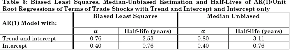
The result shown in table 5 suggests that it will take approximately 3 years and 1 month. for a unit impulse response of terms of trade shocks to half its original magnitude when taking into account a trend and intercept. On the other half, considering a case of intercept only,
Table 5: Biased Least Squares, Median-Unbiased Estimation and Half-Lives of AR(1)/Unit Root Regressions of Terms of Trade Shocks with Trend and Intercept and Intercept only AR(1) Model with: Biased Least Squares Median Unbiased
𝜶 Half-life (years) 𝜶 Half-life (years)
Trend and intercept 0.76 2.53 0.80 3.11
Intercept 0.40 0.76 0.40 0.76
Source: Authors Computation. NB: Results are presented in absolute values also the values of the Half-life after the decimal is converted to read ‘month’ in the interpretation below.
it will take approximately 9 months for a unit impulse response of terms of trade shocks to half its original magnitude. The result also shows how the least square estimates understate the true value of 𝛼 by watching the difference between the half-lives for the two estimates. This is, however, corrected using the median-unbiased estimates.
Going by the calculations and table above, the half-life of a unit shock is not infinite. Therefore, we conclude that the persistence
of terms of trade shocks in Nigeria is short-lived (temporal). This finding contradicts that of Kent and Cashin [25] who pointed out that Nigeria had a permanent (long lived) terms of trade shocks.
Results for Real Exchange Rate
Volatility (Equation [𝟔])
Cointegration Test Result
estimate the equation and test the residual for a unit root. If we do not reject the null hypothesis of a unit root, it means the
variables are not cointegrated. Otherwise, they are cointegrated.
Table 6: Cointegration Test for the Residual of Equation [𝟔] Using a Lag of One
Variable Coefficient Std. Error t-statistics Prob.
ECM(-1) -1.458625 0.331218 -4.403822 0.0002 Source: Computed by the authors.
In table 6 above, the ADF test statistics is more negative than the Engel-Granger critical value at 5 percent (-3.34), thus we reject the null hypothesis of no cointegration and conclude that there is cointegration (a long-run relationship) between real exchange rate volatility and its regressors.
This leads us to the error correction model.
Error Correction Model
By accepting that equation [6] (a distributed lag model of 1) is now a cointegrating regression, we move ahead with our error correction model.
Table 7: Error Correction Model for Equation [𝟔] Dependent Variable D(LOGRERV)
Variable Coefficient Std. Error t-statistic Prob.
Constant -0.155621 0.229900 -0.676907 0.5059
D(TOTS) 0.013348 0.005253 2.540969 0.0190
D(TOTS(-1)) 0.006353 0.004953 1.282767 0.2136
D(FD) -0.042041 0.047462 -0.885778 0.3858
D(FD(-1)) 0.089217 0.044126 2.021897 0.0561
D(TO) 0.106559 0.145133 0.734217 0.4709
D(TO(-1)) 0.283211 0.180670 1.567559 0.1319 ECM(-1) -0.878963 0.205661 -4.273842 0.0003 R-squared 0.5722
Durbin-Watson statistic 2.0764 F-statistic 4.0120 Prob(F-statistic) 0.0062
Source: Computed by the authors.
∆𝐿𝑂𝐺𝑅𝐸𝑅𝑉𝑡= 𝛾 + ∑ 𝛾𝑖∆𝑇𝑂𝑇𝑆𝑡−𝑖
1
𝑖=0
+ ∑ 𝜃𝑖∆𝐹𝐷𝑡−𝑖
1
𝑖=0
+ ∑ 𝜔𝑖∆𝑇𝑂𝑡−𝑖
1
𝑖=0
+ 𝐸𝐶𝑀𝑡−1+ 𝜈𝑡 [7]
∑ 𝛾𝑖
1
𝑖=0
=0.019701(3.8237) 𝛾0=0.013348
0.019701= 0.6775, 𝛾1 =
0.006353
0.019701= 0.32225
∑ 𝜃𝑖
1
𝑖=0
=(1.136119) 𝜃0.047176 0 =
−0.042041
0.047176 = −0.8912, 𝜃1=
0.089217
0.047176= 1.8912
∑ 𝜔𝑖
1
𝑖=0
=(2.301776) 𝜔0.38977 0=0.106559
0.38977 = 0.2734, 𝜔1=
0.283211
0.38977 = 0.7266
where the summation of the respective t ratios are in parentheses.
Table 7: Results of Diagnostic Test Statistics Prob. Breusch-Godfrey Serial Correlation LM Test (F-statistic) 1.44578 0.2603 Ramsey RESET Test (F-statistic) 0.68763 0.4168
Normality Test (Jarque-Bera) 0.08699 0.9574
The diagnostic test results reveal that we do not reject the null hypotheses of no serial correlation, no misspecification error, normally distributed error term and no heteroscedasticity. This creates a platform for us to interpret our error correction model result as shown in table 2. The coefficient of the lag of our error correction mechanism- ECM (-1), is negative (-0.878963) and statistically significance at 5 percent level of significance. This established our claim for the presence of cointegration. This implies that about 88 percent of any disequilibrium between real exchange rate volatility and its explanatory variables is corrected within the period of one year. The coefficient of determination (R2) shows that the explanatory variables in the model explained about 57 percent of the variation in a change in real exchange rate volatility. The F-statistic is significant at 5 percent level of significance, suggesting that collectively, all the variables are statistically important. Nevertheless, the impact of each independent variable is discussed below.
The result shows that the coefficient of a change in terms of trade shocks on current D (TOTS) and previous period-D(TOTS (-1), both have a positive relationship with a change in real exchange rate volatility. However, the coefficient of a change in the current period of the terms of trade shocks is statistically significant, while the coefficient of a change in the previous period of terms of trade shocks is not statistically significant at 5 percent level of significance. This implies that a percent increase in the change in the current period of terms of trade shocks on the average increases the change in the real exchange rate volatility by 0.01 percent, holding other variables constant. On the cumulative effect, a change in terms of trade shocks on a change in real exchange rate volatility is statistically significant. Therefore, the long-run impact of a percent increase in a change in terms of trade shocks on the average leads to about 0.02 percent increase in a change in real exchange rate volatility holding other variables constant. The multiplier for terms of trade shocks shows that about 68 percent of the total impact of a unit change in terms of trade shocks is felt immediately and 100 percent after one year.
The level of financial development known as financial deepening shows that the coefficient of a change in the current period of financial deepening D (FD) has a negative relationship with a change in real exchange rate volatility. On the previous period of financial deepening, the coefficient of a change in it shows a positive relationship with a change in the real exchange rate volatility. The change in the current period of financial deepening is not statistically significant, while a change in the previous period of financial development is statistically significant at 5 percent level of significance. This implies that a percent increase in the change in the previous period of financial deepening on the average, leads to an increase in the change in real exchange rate volatility by 0.09 percent, holding other variables constant. The cumulative effect of a change in financial deepening on a change in real exchange rate volatility is not statistically significant.
Trade openness which is the rate at which a country engages in international trade, shows that the coefficient of a change in the current and previous period of trade openness have positive relationships with a change in real exchange rate volatility. The coefficient of a change in trade openness for these two different time period, are not statistically different from zero at 5 percent level of significance. Therefore there is no necessity for further interpretation. However, the cumulative effect of a change in trade openness on a change in real exchange rate volatility is statistically significant. This shows that the long-run impact of a percent increase in a change in trade openness will on the average lead to 0.39 percent increase in a change in real exchange rate volatility holding other variables constant. The multiplier for trade openness shows that 27 percent of its total impact of a unit change is felt immediately and 100 percent after one year.
Conclusion
duration or persistence of terms of trade shocks, while the impact of terms of trade shocks on real exchange rate volatility followed the distributed lag model. The result shows that the persistence of terms of trade shocks is a temporal one with the duration of 3 years and 1 month and 9 months for unit root models with trend and intercept and intercept only respectively. Terms of trade shocks were found to significantly increase real exchange rate volatility immediately by up to 68 percent of a unit change in terms of trade shocks and 100 percent after one year.
The positive impact of terms of trade shocks on real exchange rate volatility implies that
Nigeria as a country has more of unfavourable terms of trade shock. To curb/mitigate this unfavourable shock, this study recommends that the export base be further diversified. Such diversification should be directed towards development of the manufacturing sector so as to add value to the raw materials which constitutes the major non-oil exports. Furthermore, the real exchange rate should be depreciated a little so as to consider/encourage low income earners to invest their hard earned money under a less uncertain environment. Finally, the temporal persistence of terms of trade shocks suggests that a little of external borrowings will not be harmful to the economy of Nigeria, since we find the shocks to die out within a short period of time.
References
1. Ezema BI (2012) Effectiveness of policy responses to terms of trade shocks in selected African countries. International Journal of Business and Management, 7(8):88-101. 2. World Bank (2003) Nigeria: Policy Option for
Growth and Stability. (Report No. 26215-NGA) Washington DC: World Bank.
3. Mordi CNO (2006) Challenges of exchange rate volatility in economic management in Nigeria. CBN Bullion, 30(3):17-25.
4. Mankiw NG (2010) Macroeconomics (7th ed.)
New York, NY: Worth publishers.
5. World Bank (2015) World Development Indicators 2015. Washington DC: World Bank.
6. Iwayemi A (1994) Perspective and problems of economic development in Nigeria: 1960-1990. Centre for Econometric and Applied Research, University of Ibadan, Ibadan. 7. Cashin P, Pattillo C (2000) Terms of Trade
Shocks in Africa: Are they short lived or long lived? (No. w00/72). International Monetary Fund.
8. Naude WA (1995) On the persistence of shocks to Ethiopia’s terms of trade: A time series analysis. Eastern African Social Science Research Review, 11(1):59-72.
9. Broda C (2004) Terms of trade and exchange rate regime in developing countries. Journal of International Economics, 63(1):31-58. 10. Andrews D, Rees D (2009) Macroeconomic
Volatility and Terms of Trade Shocks. (Research Discussion Paper No. 2009-05). Reserve Bank of Australia.
11. Black J (2002) Oxford dictionary of economics (2nd ed.) United States: Oxford University
Press.
12. Obstfeld M (1982) Aggregate spending and the terms of trade: Is there a Laursen-Metzler effect? The Quarterly Journal of Economics, 97(2):251-270.
13. Baxter M, Kouparitsas MA (2000) What Causes Fluctuations in Terms of Trade? (No. w7462). National Bureau of Economic Research.
14. Dixit AK (1989) Intersectoral capital reallocation under-price uncertainty. Journal of International Economics, 26(3):309-325. 15. Gavin M (1993) Adjusting to terms of trade
shock: Nigeria, 1972-1988. In Dombusch, R. (Eds.), Policymaking in the Open Economy, Oxford University Press.
16. Harberger AC (1950) Currency depreciation, income and the balance of trade. Journal of Political Economy, 58(1):47-60.
17. Laursen S, Metzler LA (1950) Flexible exchange rate and the theory of employment. Review of Economics and Statistics, 32(4):281-299.
18. Svensson L, Razin A (1983) The terms of trade and current account: The Harberger-Laursen-Metzler effect. Journal of Political Economy, 91(1):97-125.
uncertainty and private investment in LDCs. Review of Economics and Statistics, 85(1):212-218.
21. Ahmad AH, Pentecost EJ (2010) Terms of Trade Shocks and Economic Performance under Different Exchange Rate Regimes. (Discussion papers No. w 2010-08). Department of Economics, Loughborough University.
22. Funke N, Granziera E, Imam P (2008) Terms of Trade Shocks and Economic Recovery. (No. w08/36). International Monetary Fund. 23. Jimoh A (2006) The effects of trade
liberalization on real exchange rate: Evidence from Nigeria. Journal of Economic Cooperation, 27(4):45-62.
24. Andrews DWK (1993) Exactly median-unbiased estimation of first order
Econometrica, 61(1):139-165.
25. Kent C, Cashin P (2003) The Response of the Current Account to Terms of Trade Shocks: Persistence Matters. (No. w03/143). International Monetary Fund.
26. DeJong DN, Nankervis JC, Savin NE, Whiteman CH (1992) Integration versus trend stationarity in times series. Econometrica, 60(2):423-433.
27. Gujarati DN, Porter DC (2009) Basic econometrics (5th ed.). New York: McGraw