ShookSa_unc_0153D_19185.pdf

(1)

INVERSE PROBABILITY WEIGHTING AND OUTCOME REGRESSION APPROACHES IN CAUSAL INFERENCE AND SURVEY SAMPLING

Bonnie E. Shook-Sa

A dissertation submitted to the faculty of the University of North Carolina at Chapel Hill in partial fulfillment of the requirements for the degree of Doctor of Public Health in the Department of

Biostatistics in the Gillings School of Global Public Health.

Chapel Hill 2020

(2)

(3)

ABSTRACT

Bonnie E. Shook-Sa: Inverse Probability Weighting and Outcome Regression Approaches in Causal Inference and Survey Sampling

(Under the direction of Michael G. Hudgens)

Survey sampling and causal inference share much of the same theoretical foundation. Both fields commonly use estimation methods that rely on randomization-based or prediction-based inferential paradigms, and inverse-probability weighting (IPW) and outcome regression methods are common in both fields (Lohr, 2010; Hern´an and Robins, 2020). IPW estimators are used in conjunction with marginal structural models (MSMs) to estimate causal effects from observational studies by controlling for confounding. The parametric g-formula is an outcome regression approach utilized to make causal estimates in the presence of confounding by directly modeling the outcome as a function of the exposure and confounding variables and then integrating over the distribution of the confounders. IPW estimators are fundamental in survey sampling, as they appropriately account for each unit’s probability of selection within a finite population and can be further adjusted to account for nonresponding units and undercoverage of the target population. Under a prediction-based inferential paradigm, outcome regression is used to impute outcomes for units not selected into the sample based on data from sampled units.

(4)

A common technique for sample size determination for complex sample surveys is to make use of the design effect, the ratio of the variance of an estimator under a complex sample design to the variance of the estimator under a simple random sample (Kish, 1965). Design effects allow researchers to calculate sample sizes under the simpler design and then inflate them to account for the use of weights in the analysis. In our second paper, we extend the theory of design effects to causal inference. The design effect approximation can be used to design causal studies that will be analyzed using MSM with IPW to control for confounding.

(5)

(6)

ACKNOWLEDGEMENTS

I would like to thank my dissertation advisor, Dr. Michael Hudgens, for his guidance throughout the dissertation process and for empowering me to reach my full potential. He has inspired me to be a better statistician in both methods research and in application. Thank you also to my dissertation committee Dr. Stephen Cole, Dr. John Preisser, Dr. David Rosen, and Dr. Donglin Zeng for their valuable feedback and helpful suggestions that have strengthened this research.

The research in Chapter 2 was supported by NIH grant R01 AI129731. Dr. David Rosen and Andrew Kavee are co-authors on this paper. Thanks also to Dr. Phillip Kott at RTI International for his helpful suggestions.

The research in Chapters 3 and 4 was supported by NIH grant R01 AI085073. The research in Paper 3 was funded in part through Developmental funding from the University of North Carolina at Chapel Hill Center For AIDS Research (CFAR), an NIH funded program P30 AI050410. The authors thank Dr. Stephen Cole, Noah Greifer, Shaina Alexandria, Bryan Blette, Kayla Kilpatrick, and Dr. Jaffer Zaidi for their helpful suggestions.

(7)

Aouizerat and Phyllis Tien), U01-HL146242; Los Angeles CRS (Roger Detels), U01-HL146333; Metropolitan Washington CRS (Seble Kassaye and Daniel Merenstein), U01-HL146205; Miami CRS (Maria Alcaide, Margaret Fischl, and Deborah Jones), U01-HL146203; Pittsburgh CRS (Jeremy Martinson and Charles Rinaldo), U01-HL146208; UAB-MS CRS (Mirjam-Colette Kempf and Deborah Konkle-Parker), U01-HL146192; UNC CRS (Adaora Adimora), U01-HL146194. The MWCCS is funded primarily by the National Heart, Lung, and Blood Institute (NHLBI), with additional co-funding from the Eunice Kennedy Shriver National Institute Of Child Health & Human Development (NICHD), National Human Genome Research Institute (NHGRI), National Institute On Aging (NIA), National Institute Of Dental & Craniofacial Research (NIDCR), National Institute Of Allergy And Infectious Diseases (NIAID), National Institute Of Neurological Disorders And Stroke (NINDS), National Institute Of Mental Health (NIMH), National Institute On Drug Abuse (NIDA), National Institute Of Nursing Research (NINR), National Cancer Institute (NCI), National Institute on Alcohol Abuse and Alcoholism (NIAAA), National Institute on Deafness and Other Communication Disorders (NIDCD), National Institute of Diabetes and Digestive and Kidney Diseases (NIDDK). MWCCS data collection is also supported by UL1-TR000004 (UCSF CTSA), P30-AI-050409 (Atlanta CFAR), P30-AI-050410 (UNC CFAR), and P30-AI-0277 67 (UAB CFAR). Thanks to Dr. Andrea Knittel, Dr. Andrew Edmonds, Catalina Ramirez, and Dr. Adaora Adimora for contributions to the work in Chapter 4.

(8)

TABLE OF CONTENTS

LIST OF TABLES . . . xii

LIST OF FIGURES . . . xiv

CHAPTER 1: INTRODUCTION AND LITERATURE REVIEW . . . 1

1.1 Introduction . . . 1

1.2 Causal Inference . . . 2

1.2.1 Inferential Paradigms . . . 2

1.2.2 IPW and Outcome Regression Approaches . . . 3

1.2.2.1 IPW Estimation . . . 3

1.2.2.2 Outcome Regression Approaches . . . 5

1.2.2.3 Doubly Robust Estimation Approaches . . . 5

1.3 Survey Sampling . . . 6

1.3.1 Inferential Paradigms . . . 6

1.3.2 IPW and Outcome Regression Approaches . . . 8

1.3.2.1 IPW Estimation . . . 8

1.3.2.2 Outcome Regression Approaches . . . 10

1.4 Design Effects . . . 11

1.5 Issues Surrounding the Analysis of Count Data . . . 13

1.5.1 Overdispersion . . . 13

1.5.2 Data Heaping . . . 14

1.6 Motivating Examples . . . 14

(9)

1.6.2 Women’s Interagency HIV Study . . . 15

CHAPTER 2: SURVEY SAMPLING APPROACHES TO ESTIMATE THE NUMBER OF HIV-POSITIVE PERSONS IN NORTH CAROLINA JAILS . . . 16

2.2 Methods . . . 17

2.2.1 Record Linkage . . . 17

2.2.2 Preliminary Data Description . . . 19

2.2.3 Estimation . . . 20

2.2.3.1 Outcome Regression . . . 21

2.2.3.2 Weight Calibration . . . 22

2.3 Simulation Study . . . 25

2.4 Preliminary Data Results . . . 30

2.4.1 Outcome Regression . . . 30

2.4.2 Weight Calibration . . . 31

2.5 Discussion . . . 36

CHAPTER 3: DON’T LET CONFOUNDING CONFOUND YOU: POWER AND SAMPLE SIZE FOR MARGINAL STRUCTURAL MODELS . . . 37

3.2 The Design Effect . . . 40

3.2.1 Preliminaries . . . 40

3.2.2 The Design Effect for a Single Causal Mean . . . 41

3.3 Sample Size Calculations using the Design Effects . . . 43

3.4.1 Simulation Scenarios . . . 45

3.4.2 Sample Size Calculation . . . 45

(10)

3.4.2.3 Na¨ıve Sample Size Calculations . . . 47

3.4.3 Evaluation . . . 48

3.5 Practical Considerations . . . 51

CHAPTER 4: CAUSAL INFERENCE FROM OBSERVATIONAL DATA FOR COUNT OUTCOMES . . . 56

4.2 Methods . . . 58

4.2.1 Preliminaries . . . 58

4.2.2 MSM with IPTW . . . 58

4.2.3 Parametric g-formula . . . 60

4.2.4 Doubly Robust Estimation . . . 62

4.2.5 Data Heaping . . . 64

4.2.5.1 MSM with IPTW . . . 65

4.2.5.2 Parametric g-formula . . . 66

4.2.5.3 Doubly Robust Estimation . . . 67

4.3.1 Without Data Heaping . . . 68

4.3.2 With Data Heaping . . . 70

4.4 Example: Women’s Interagency HIV Study . . . 75

APPENDIX A: TECHNICAL DETAILS FOR CHAPTER 3 . . . 81

A.1 Proofs of Propositions . . . 81

A.1.1 Proposition 3.1 . . . 81

A.1.2 Proposition 3.2 . . . 83

(11)

APPENDIX B: TECHNICAL DETAILS FOR CHAPTER 4 . . . 85

B.1 Supplemental Tables . . . 85

B.2 Proofs of Propositions . . . 87

B.2.1 Proposition 4.1 . . . 87

(12)

LIST OF TABLES

2.1 Simulation Summary Results,R= 1000Simulations . . . 29 2.2 Parameter Estimates for Multivariable and Single Variable Prediction

Models, Outcome Regression . . . 32 2.3 Estimated Number of HIV-positive Persons Incarcerated in Jails in the

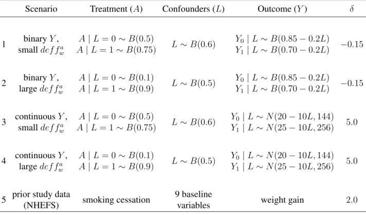
10 Largest and 10 Smallest Counties, Outcome Regression . . . 33 2.4 County Characteristics by Response Status . . . 34 2.5 Parameter Estimates for Weight Calibration Model . . . 35 3.1 Five simulation scenarios. Scenarios 1-4 demonstrate use of the

de-sign effect when no prior study data are available, and Scenario 5 demonstrates use of the design effect with prior study data.X ∼B(p)

indicates that a random variableXfollows the Bernoulli distribution

with probability of success equal top. . . 45 3.2 Variances, approximated design effects, approximated adjusted

vari-ances, and required sample sizes for simulation scenarios by treatment. . . 48 3.3 Results of the simulation study by scenario acrossR= 2000samples.

Empirical powerndef f andnrctare the proportions of simulated sam-ples in which the p-values for testingH0 :β1 = 0versusH1 :β1 6= 0

were less thanα= 0.05for the following MSM:E(Yai) = β0+β1ai,

based on sample sizesndef f andnrct, respectively, from Table 3.2 . . . 51 4.1 Results of the simulation study by distribution and method acrossR=

1000samples with correct model specification, n = 800. Empirical bias, ASE, ESE, SER, and empirical 95% confidence interval coverage

calculated for theCRR. . . 70 4.2 Results of the simulation study by distribution and method across

R = 1000samples with one or both models misspecified, n = 800. Empirical bias, ASE, ESE, SER, and empirical 95% confidence interval

coverage calculated for theCRR. . . 73 4.3 Results of the data heaping simulation study by method acrossR =

1000samples with correct model specification,n = 800. All heaping estimators and the na¨ıve PG and DR estimators assume a Poisson distribution. Empirical bias, ASE, ESE, SER, and empirical 95%

(13)

4.4 Results of the data heaping simulation study by method acrossR = 1000 samples with one or both models misspecified, n = 800. All estimators assume a Poisson distribution. Empirical bias, ASE, ESE,

SER, and empirical 95% confidence interval coverage calculated for theCRR. . . 74 4.5 Estimated causal rate ratios, estimated standard errors, and Wald 95%

confidence intervals for the effect of incarceration on the number of male sexual partners in the subsequent six months by method and

assumed parametric distribution, WIHS 2007-2017 . . . 78 B1 Results of the simulation study by distribution and method acrossR=

1000samples with correct model specification,n = 2000. Empirical bias, ASE, ESE, SER, and empirical 95% confidence interval coverage

calculated for theCRR. . . 85 B2 Results of the simulation study by distribution and method across

R = 1000samples with one or both models misspecified,n = 2000. Empirical bias, ASE, ESE, SER, and empirical 95% confidence interval

(14)

LIST OF FIGURES

2.1 Availability of Jail Rosters by NC County . . . 18 2.2 Density Plots for Outcome Regression vs. Weight Calibration,R =

1000Simulations . . . 28 2.3 Predicted vs. Actual Proportion of Defendants who were Incarcerated,

n= 26Counties with Publicly-Available Jail Rosters . . . 31 2.4 Estimated Number of HIV+ Persons Incarcerated in NC Jails (nˆI,N C)

and 95% Confidence Intervals based on Outcome Regression and

Weight Calibration . . . 35 3.1 Examples of weight distributions for various approximated design

effects. Distributions were generated by taking the reciprocals of Na = 1000random draws from beta distributions with mean 0.5 and

shape parameters set to achieve the desired design effect. . . 53 4.1 Density plot of the true distribution of partners with a histogram of the

reported (heaped) number of partners for a single simulation,n= 800 . . . 71 4.2 Distribution of partners during the six months following the study

period reported by WIHS participants in the analytic sample: 0-4

(15)

CHAPTER 1: INTRODUCTION AND LITERATURE REVIEW

1.1 Introduction

Survey sampling and causal inference share much of the same theoretical foundation, and inverse-probability weighting (IPW) and outcome regression approaches are common in both fields. This dissertation focuses on applications and extensions of IPW and outcome regression approaches in the fields of causal inference and survey sampling. Chapter 2 proposes and compares survey sampling methods utilizing IPW and outcome regression for estimating the number of HIV-positive persons incarcerated in NC jails when study data are available only for a nonrandom subset of counties. Chapter 3 extends the theory of design effects from survey sampling to causal inference to allow for design of studies that will be analyzed using MSM with IPTWs. Chapter 4 provides a theoretical justification for the use of MSMs, the parametric g-formula, and doubly robust estimators for count outcome and proposes methods that account for overdispersion and data heaping.

(16)

1.2 Causal Inference

1.2.1 Inferential Paradigms

Causal inference aims to move beyond measures of association to estimate causal effects between variables. Neyman (1923) introduced the potential outcomes framework, and Rubin (1974; 1977; 1978) popularized this framework in the 1970s. This led to the Neyman-Rubin causal model, which serves as the foundation of causal inference. Under the potential outcomes framework, for a dichotomous treatmentAthe potential outcomeYa_{represents the outcome that would be observed} under treatment assignmentA=a,a∈ {0,1}. In causal inference, the estimands are functions of the potential outcomes. For each participant, only the potential outcome associated with the realized treatment status is observed, and the other (counterfactual) outcome is unobserved. This leads to what Holland (1986) calls the fundamental problem of causal inference, which is a missing data problem.

Two of the inferential paradigms commonly employed in causal inference are randomization-based and prediction-randomization-based (or large sample frequentist) inference. Under randomization-randomization-based inference, the potential outcomes are commonly viewed as fixed characteristics of a finite population, and the only random component is the treatment assignmentAfor each participant. Expectations and variances are calculated based on all possible randomizations of treatment assignments. Neyman (1923) provides unbiased estimators for the average causal effect under the randomization-based paradigm along with their variance estimators.

The prediction-based paradigm relies on a large-sample frequentist perspective. LetAirepresent the binary treatment status for participanti(Ai = 1means participantireceived treatment,Ai = 0 means participant i did not receive treatment), Li be a vector of baseline covariates measured

(17)

1.2.2 IPW and Outcome Regression Approaches

Standard statistical methods cannot be used to calculate causal effects from observational data when confounding is present, as measures of association differ from the causal effects of interest. Two methods commonly employed to calculate causal estimates in the presence of confounding are marginal structural models (MSMs) with IPW and the parametric g-formula, which is an outcome regression approach.

Both methods rely on three identifiability conditions: causal consistency, positivity, and con-ditional exchangeability. Causal consistency defines the observed outcomeY as a function of the potential outcomes and treatment assignment: Y =AY1_{+ (1}₋_A₎_Y0 _{(Rubin, 1980; Gibbard and}

William, 1981; Cole and Frangakis, 2009; Pearl, 2010). Positivity states that there is a non-zero probability of each level of treatmentAfor all combinations ofAandLin the population (Cole and Frangakis, 2009; Hern´an and Robins, 2020). Under conditional exchangeability, it is assumed that Ya _⊥ _A _| _L_,_a _{∈ {}₀_,₁_}_{. That is, the potential outcomes are independent of the treatment} assignment given the set of measured confounding variablesL. This assumption is also referred to as the assumption of no unmeasured confounding (Hern´an and Robins, 2020).

1.2.2.1 IPW Estimation

The propensity score for each participant is defined asei =P r(Ai = 1|Li), the probability

that participantireceived treatmentA= 1conditional on covariatesLi (Rosenbaum and Rubin,

1983). The inverse-probability of treatment weight (IPTW) is equal toWi =Aie−i 1+ (1−Ai)(1− ei)−1. Weighting individuals byWicreates a pseudo-population in which confounding by variables Lis not present, which allows for the estimation of causal effects (Robins et al., 2000).

(18)

score and the observed treatment assignment:Wî =I(Ai = 1)ê−i 1+I(Ai = 0)(1−êi)−1, where I(Ai =a)is a{0,1}treatment indicator for participanti. Weighted estimating equations are then used to regress the observed outcomeY on treatmentAwith weightsWˆ. Under the assumptions of causal consistency, positivity, and conditional exchangeability, causal effects are identifiable because within the weighted populationE(Y |A=a) =E(Ya _|_A₌_a_{) =}_E₍_Ya₎_for_a_{∈ {}₀_,₁_}_. When the weight model is correctly specified the average causal effect,E(Y1)−E(Y0), can be consistently estimated as a difference in Hájek estimators for the two causal means (Lunceford and Davidian, 2004):

[

ACE = ˆµ1₋_µˆ0 ₌ Pn

i=1WˆiYiI[Ai = 1]

Pn

i=1WˆiI[Ai = 1]

− Pn

i=1WˆiYiI[Ai = 0]

Pn

i=1WˆiI[Ai = 0]

Lunceford and Davidian (2004) show that the empirical sandwich variance estimator provides a consistent estimate for the asymptotic variance of the estimated average causal effect when the weight model is correctly specified and that the asymptotic variance of ACE[ is Σ = E{(Y1 ₋

µ1₎2_e−1_{+ (}_Y0₋_µ0₎2₍₁₋_e₎−1_}_{when the weights are treated as fixed. Furthermore, Lunceford and}

Davidian (2004) show that treating the weights as fixed leads to a conservative variance estimate, as the asymptotic variance when the weights are appropriately treated as estimated is less thanΣ.

(19)

1.2.2.2 Outcome Regression Approaches

The parametric g-formula is an outcome regression approach used in causal inference that is an alternative to MSMs with IPWs. Standardization is a common analytic technique in epidemiology research (see, for example Rothman, 2012, pages 188-192). Robins (1986) introduced the parametric g-formula as a type of standardization that allows for the estimation of causal effects by directly modeling the outcome as a function of the exposure and confounding variables and then integrating over the distribution of the confounding variables.

More specifically, under the assumptions of conditional exchangeability and causal consistency, E[Ya_|_L₌_l_{] =}_E_[_Ya_|_L₌_l_{, A}₌_a_{] =}_E_[_Y _|_L₌_l_{, A}₌_a_]_{. The final quantity is identifiable} from the data and can be estimated using standard parametric models (e.g. linear regression, logistic regression) (Hern´an and Robins, 2020). Causal means are then estimated using the law of total probability and integrating over the distribution ofL,E[Ya] =R E[Y |L=l, A=a]dFL(l). This is typically done empirically by taking the average of theEˆ[Y | L= l, A =a]for the observed data (Hern´an and Robins, 2020).

The parametric g-formula can lead to more stable and efficient estimates compared to MSM with IPW (Daniel et al., 2013). The drawbacks of the parametric g-formula are that it requires correct specification of the outcome regression model (i.e., correctly specifying the relationship between the outcome and the exposure and confounding variables) and that it can be problematic in longitudinal settings due to a phenomenon known as the “g-null paradox”. Under the g-null paradox, when there is treatment-confounder feedback, the null hypothesis of no treatment effect will be rejected with probability approaching one under the null given enough data (Hern´an and Robins, 2020; Robins, 1986).

1.2.2.3 Doubly Robust Estimation Approaches

(20)

et al., 2011). Because the relationships between the exposure, outcome, and confounding variables are typically unknown in observational settings, doubly robust estimators afford some protection against misspecification of these models (Funk et al., 2011). While in practice all models are at least partially misspecified, Bang and Robins (2005) note that doubly robust estimators allow for minimal bias when either the weight or outcome model is nearly correct, giving the researcher two chances to get close to correct specification. Lunceford and Davidian (2004) consider the doubly robust estimators below, proposed by Robins et al. (1994), for the causal means of two binary treatment groups.

ˆ

E[Y1] =n−1 n

X

i=1

AiYi− {Ai−π(Li,γˆ)}m1(Li,βˆ1) π(Li,ˆγ)

and

ˆ

E[Y0] =n−1 n

X

i=1

(1−Ai)Yi+{Ai−π(Li,γˆ)}m0(Li,βˆ0)

1−π(Li,γˆ)

where π(Li,γˆ) is the estimated propensity score for participant i from the weight model and

ma(Li,βˆa) is the predicted potential outcome for participanti from the parametric g-formula

model. These estimators combine the MSM and parametric g-formula estimators and are consistent and asymptotically normal when either model is correctly specified (Lunceford and Davidian, 2004). An alternative doubly robust estimator is constructed by incorporating the reciprocal of the estimated propensity score,ˆe−1_{as a covariate in the outcome regression model (Scharfstein et al., 1999; Bang}

and Robins, 2005).

1.3 Survey Sampling

1.3.1 Inferential Paradigms

(21)

treated as fixed quantities associated with the finite population and the only random component is which elements of the finite population are selected into the sample (Lohr, 2010, page 54). As in the randomization-based approach to causal inference described above, expectations and variances are calculated based on all possible randomizations. In survey sampling, these randomizations are the possible samples that could have been selected. These methods are sometimes referred to as unconditional, as they rely on averages over all possible samples and are not conditioned on the observed sample (Lavrakas, 2008).

An alternative approach to sample survey estimation is the prediction-based (or model-based) inferential paradigm. Royall (1970; 1976; 1978) was one of the early pioneers of the prediction-based paradigm within survey sampling, proposing models prediction-based on a superpopulation perspective and the use of auxiliary data for analyzing survey data. Under the prediction-based approach, the outcomes themselves are considered random variables that follow a model, and the finite population is thought of as a single realization of these random variables from a superpopulation (S¨arndal et al., 1978). Data from the observed sample is used to predict the unobserved values from the non sampled members of the finite population, and variances are estimated using standard parametric modeling theory (S¨arndal et al., 2003; Bolfarine and Zacks, 1992; Lohr, 2010, page 148). These methods can be more efficient than randomization-based methods when the model is correctly specified, but can lead to substantially biased estimates when the model is incorrectly specified (Hansen, 1987).

(22)

the double-robustness property. The GREG remains design-unbiased even when the regression model is misspecified (Cassel et al., 1976; S¨arndal et al., 2003; Kang and Schafer, 2007). The Generalized Exponential Model (GEM) is a generalization of the GREG and is further discussed in Section 1.3.2.1. Proponents of randomization assisted model based inference argue that inference should be based on the realized sample rather than across all possible samples, so this alternative framework uses prediction-based theory but brings features of the sample design (e.g. stratification and clustering) into the modeling framework (S¨arndal, 2010; Kott, 2005).

1.3.2 IPW and Outcome Regression Approaches

IPW and outcome regression approaches are common in survey sampling. We focus on weight calibration estimators, specifically the GEM, under the randomization assisted model based inferential paradigm and the use of outcome regression to impute missing data for units that were not selected under the prediction-based paradigm. LetN be the finite population size andnrepresent the sample size.

1.3.2.1 IPW Estimation

Under the randomization-based paradigm, weightswiare defined as the reciprocal of each unit i’s probability of selection. These are commonly referred to as base weights (Valliant et al., 2013,

pages 311-314). Base weights can be further adjusted using auxiliary data under the model assisted or randomization assisted model based paradigms to account for nonresponding units or sampling frame undercoverage of the target population (Kott, 2006; Kott and Day, 2014; Valliant et al., 2013, Ch 13-14).

(23)

study (Kott and Liao, 2015). Calibration models also reduce the variance of an estimated total compared to estimation based on uncalibrated weights when the outcome of interest is correlated with calibration variables (Deville and S¨arndal, 1992).

A GEM is a type of weight calibration model used to calibrate the sample to known population totals (Folsom and Singh, 2000). Under this model, the weight adjustment for each participating unitiis defined as:

θi(xi,γ) =

li(ui−ci) +ui(ci−li) exp(aixiγ)

(ui−ci) + (ci−li) exp(aixiγ)

where xi is a 1×p vector of calibration variables for participant i, where p is the number of calibration variables in the model;liandui are specified by the analyst and determine the lower and upper bounds of the adjustments, respectively; ci is a centering constant for the model; and ai is a function ofli,ui, andci (Folsom and Singh, 2000; RTI International, 2012). Let ri be a response indicator for participanti: ri = 1if participantiresponded, 0 otherwise. The specified lower and upper bounds put constraints on the assumed response model. Specifying a lower bound of 0 implicitly models each participant’s probability of response as an exponential function of the calibration variables, while specifying a lower bound of 1 implicitly assumes a logistic relationship (Kott, 2006; Kott and Liao, 2012). Let Tx be ap×1vector of population totals known for the finite population. That is,Tx =PN_i₌₁xTi. Then, weight adjustments for each responding unit are

obtained by solving the following set of calibration equations forγusing Newton-Raphson:

sp(γ) = N

X

i=1

xT_iwiriθi(xi,γ)−Tx =0

(24)

and Folsom, 2000; RTI International, 2012). Kott and Liao (2012) discuss the doubly robust properties of the GEM estimator, as it provides consistent estimates when either the implied response model or the linear predictor model is correctly specified.

Utilizing weight calibration provides the researcher control over the weight adjustments while adjusting for sample undercoverage or nonresponse. This method appropriately treats the weights as estimated when calculating variances instead of treating adjusted weights as fixed or known (Shook-Sa et al., 2017). The disadvantage of weight calibration models are that results are based on asymptotic theory, so unbiasedness and confidence interval coverage might not hold in small samples (Kott, 2006).

1.3.2.2 Outcome Regression Approaches

Under the prediction-based inferential paradigm, data from the observed sample of sizenis used to predict theN −n unobserved values from the non-sampled units of a finite population (Lohr, 2010, page 148; Royall, 1976; S¨arndal et al., 2003, pages 533-534). For example, for a continuous outcomeY, the following linear regression model can be fit for sampled and responding units: Yi =xiβ+, where∼N(0, σ2). Predicted values from the model are used to estimate the outcome of interest for non-sampled units of the finite population, and finite population totalsT are estimated as the sum of the observed and predicted values in the population. Assume that units are ordered such thati= 1, ..., nwere selected and unitsi=n+ 1, ..., N were not selected. Then the estimated population totalTˆcan be defined as follows, and variances can be computed using using standard linear model theory (Royall, 1976; Royall and Cumberland, 1978; Lohr, 2010, page 148; S¨arndal et al., 2003, pages 533-534; Bolfarine and Zacks, 1992).

ˆ

T =

n

X

i=1

Yi+ N

X

j=n+1 ˆ

Yj

(25)

148). However, bias can be significant when the model is not correctly specified (Hansen, 1987; S¨arndal et al., 2003, page 535).

1.4 Design Effects

Weighted estimators are fundamental in survey sampling, and methods have been developed to quantify the effect of weighting on the precision of resulting estimates. Kish (1965, page 257) introduced the design effect, which is the ratio of the variance of an estimator under a complex sample design to the variance of the estimator under a simple random sample. When observations are independent, the design effect simplifies to the design effect due to weighting (def fw), or the unequal weighting effect (Kish, 1992). Letwi represent the sampling weight for theithparticipant andnbe the sample size. The design effect due to weighting can be calculated as:

def fw = nPn

i=1wi 2

{Pn i=1wi}2

The design effect is interpreted as an estimator’s increase in variance due to differential weights across participants. While this metric was theoretically motivated by a comparison of variance estimators under different stratification allocations, it is commonly applied to all types of complex sample designs in which sample members have different probabilities of selection (Valliant et al., 2013, page 375). Gabler et al. (1999) provided a justification for how Kish’s design effect applies to model-based estimators.

The design effect is commonly utilized in sample size calculations through the use of the effective sample size. The effective sample size is equal to the observed sample size divided by the design effect. It can be interpreted as the sample size under simple random sampling that produces the same variance as the sample selected under the complex design (Valliant et al., 2013, page 5).

(26)

that would be achieved if sampling had been conducted directly from the distribution of interest (Kong et al., 1994). Kong (1992) approximates the effective sample size as the observed sample size divided bydef fw.

Within causal inference,def fw has been used to quantify the loss of statistical precision due to weighting (McCaffrey et al., 2004, 2013), but the design effect has not previously been theoretically justified for causal methods and has not been used in power and sample size calculations. For the purposes of study design, the advantages of the design effect are that it is (1) outcome invariant and (2) allows the sample size under the complex design to be translated into an equivalent sample size under a simpler design. The former implies that the approximated design effect depends only on the participants’ weights and is constant across outcomes. The latter means that oncedef fw is known or approximated, it can be used in power and sample size calculations along with the simpler assumptions needed to design a study without weights.

(27)

1.5 Issues Surrounding the Analysis of Count Data

Two common issues that can complicate the analysis of self-reported count data are the presence of overdispersion in the data and data heaping. Analytic approaches are needed to account for the presence of overdispersion or data heaping when the estimand is a count or a function of counts.

1.5.1 Overdispersion

The Poisson distribution takes on non-negative integer values and is often used to model the number of events that occur in a specific time or place (Weisberg, 2005, page 271). Count data are commonly modeled using Poisson generalized linear models (GLMs), in which the rate parameter is modeled as a linear function of predictorsX through the link function (McCullagh and Nelder., 1989, Ch 6). That is, we assume thatY ∼ P oisson(λ)and model the canonical (log) ofλas a linear function of covariates: log(λ) =Xβ.

Because the Poisson distribution has a single parameterλ such thatE(Y) = V ar(Y) = λ, count data commonly exhibit overdispersion. Overdispersion occurs when variation in the data exceeds the expected variation based on an assumed Poisson distribution (i.e.,V ar(Y)> E(Y)) (Agresti, 2002, page 130).

Negative binomial models are one alternative when data exhibit overdispersion. The negative binomial distribution has two parameters, withE(Y) = λandV ar(Y) =λ+λ2_{θ. Because the}

negative binomial has an additional parameterθ(the dispersion parameter), it allows the variance to exceed the mean (Agresti, 2002, page 131).

(28)

similar interpretations to those in the Poisson and negative binomial GLMs (Long et al., 2014; Preisser et al., 2016).

1.5.2 Data Heaping

Self-reported count data frequently exhibit a form of measurement error known as data heaping, where reported counts are rounded to different levels of precision (Wang and Heitjan, 2008). This phenomenon is commonly observed when collecting self-reported retrospective counts or measures of duration, including cigarette usage (Klesges et al., 1995), duration of breastfeeding (Singh and Folsom, 2000), and number of sexual partners (Wiederman, 1997; Roberts and Brewer, 2001). Data heaping is often attributed to cognitive processes in respondents, including choosing round numbers or approximations (digit preference) or using estimation methods to aid in recall (Roberts and Brewer, 2001). Data heaping distorts the true underlying distribution of counts and can thus lead to biased inference and increased variance (Wang and Heitjan, 2008; Cummings et al., 2015).

Methods have been proposed both to detect and account for heaping. Roberts and Brewer (2001) propose a measure and test to quantify the amount of heaping in discrete data. Heitjan and Rubin (1990) propose multiple imputation methods to account for data heaping. Singh et al. (1994) present a smoothing method for heaped time-to-event data. Bayesian mixture models are another way to account for heaping in observed data (Wright and Bray, 2003; Wang and Heitjan, 2008). Cummings et al. (2015) present an interval-censored likelihood approach for accounting for heaped count data.

1.6 Motivating Examples

(29)

1.6.1 Estimating the Number of HIV-Positive Persons in North Carolina Jails

The methods in Chapter 2 were developed to estimate the number of HIV-positive persons incarcerated in North Carolina (NC) jails overall and within each of the 100 counties over a fixed period of time. NC does not maintain a list of HIV-positive persons incarcerated in its jails. To estimate the size of this population, jail incarceration records, statewide court records, and confidential statewide health department records of persons living with HIV will be linked. This record linkage process will provide estimates for the number of HIV-positive persons incarcerated in the 26 counties with available jail incarceration data, but not for the remaining 74 counties. The characteristics of the counties with publicly-available data likely differ from those without publicly-available data, so appropriate statistical methods are needed generalize these results to the entire state of NC.

1.6.2 Women’s Interagency HIV Study

(30)

CHAPTER 2: SURVEY SAMPLING APPROACHES TO ESTIMATE THE NUMBER OF HIV-POSITIVE PERSONS IN NORTH CAROLINA JAILS

2.1 Introduction

Calculating estimates for rare or dynamic populations is challenging when no single data source contains all information necessary for estimation. A lack of a viable sampling frame further precludes the use of conventional methods for estimating the size and characteristics of a rare or ever-changing population. Record linkage techniques allow for multiple data sources to be combined, which can facilitate indirect estimation of the target population (Harron et al., 2017; Qayad and Zhang, 2009; St. Sauver et al., 2011). However, when record linkage results in missing data, methods are needed to generalize findings based on linked records to the target population (Bohensky et al., 2010; Ford et al., 2006; Harron et al., 2014; Judson et al., 2013).

The goal of this study is to develop and evaluate methods to account for missing data following record linkage to estimate the number of HIV-positive persons incarcerated in the state of North Carolina (NC) jails overall and within each of the 100 counties over a fixed period of time. Estimates of HIV within and across county jails in the state could be used by jail administrators as well as by local and state public health officials in efforts to ensure the availability of adequate medical resources to treat HIV during periods of jail incarceration and to support incarcerated persons’ health needs as they are released and return to the community.

(31)

HIV-positive persons incarcerated in jails in the 26 counties with available jail incarceration data. The characteristics of the counties with publicly-available data likely differ from those without publicly-available data, so care must be taken when generalizing these results to the entire state of NC.

This paper uses preliminary study data to develop methods for estimating the number of persons incarcerated in NC jails living with HIV. The findings from this methods evaluation will be used to determine the primary analytic methods that will be applied to the final dataset once data collection and linkage are complete. Two methods are considered, both of which provide estimates for the total number of persons incarcerated in NC jails living with HIV, and one of which also provides county-level estimates within the 74 counties without publicly-available jail rosters. Both methods use sampling inference approaches that leverage county-level characteristics, either via outcome regression or weight calibration modeling. In Section 2.2 both methods are presented. Section 2.3 describes a simulation study assessing and comparing these methods based on bias and precision, and Section 2.4 provides an illustration of the two approaches based on preliminary study data. Section 2.5 concludes with a discussion of the results and outlines the limitations of our study.

2.2 Methods

2.2.1 Record Linkage

To generate estimates of the number of people in NC jails living with HIV, the following datasets will be linked: jail incarceration records, state court records, and confidential NC health department records of persons in the state known to be living with HIV. A database of jail incarceration records is being created using a technique called webscraping, in which, several times a day, automated ‘bots’ collect individual-level incarceration data from jail rosters published on county jail websites.

(32)

Figure 2.1: Availability of Jail Rosters by NC County

State criminal court records are being obtained from the NC Administrative Office of the Courts. These records include variables such as defendants’ full names, DOBs, partial social security numbers (SSNs), and the county court system in which defendants’ cases will be adjudicated. Over a three-month period, there are over 400,000 defendant-level records in the 26 counties with online inmate-level rosters and nearly 800,000 defendant-level records for the entire state of NC.

Finally, the NC State Health Department maintains a confidential database of all living persons who were diagnosed with HIV in the state. Among other variables, this database includes patients’ full names, DOBs, SSNs, and dates of HIV diagnoses. This database tracks persons with positive HIV tests and persons accessing HIV services in NC.

(33)

Review Board at the University of North Carolina at Chapel Hill reviewed and approved the study protocol (IRB # 17-0946).

2.2.2 Preliminary Data Description

To avoid using final study data to develop the statistical analysis plan, methods development is conducted using preliminary study data based on three months of linked jail-court records. Public health records have not yet been linked to the individual level jail-court records, so preliminary data includes the total number of defendants in each county over a three-month period but not the number of HIV-positive defendants or the number of HIV-positive persons incarcerated in the 26 counties with publicly-available jail rosters.

For the purposes of developing a preliminary data file for use in methods evaluation, the number of HIV-positive defendants in each county was approximated by multiplying the number of defendants by the estimated prevalence of HIV among the defendant population in each county. The estimated prevalence of HIV in each NC county was obtained by dividing the count of residents who were HIV-positive (North Carolina HIV/STD/Hepatitis Surveillance Unit, 2017) by the estimated number of county residents in 2016 from the US Census Bureau (U.S. Census Bureau Population Division, 2018). The assumed HIV prevalence among defendants was set equal to the county prevalence multiplied by five. This multiplier was chosen to reflect the approximate increased risk of HIV among persons entering the criminal justice system, based on the known prevalence of HIV in NC and the estimated prevalence among those entering the criminal justice system (Wohl et al., 2013).

(34)

2.2.3 Estimation

The estimands are the total number of HIV-positive persons incarcerated in jails over a fixed period of time (1) in NC (nI,N C) and (2) within each of the 100 counties in NC (nI,i, i = 1, ..,100). Within each countyi, the number of HIV-positive persons who were incarcerated equals the number of HIV-positive defendants (nD,i) multiplied by the proportion of HIV-positive defendants in county iwho were incarcerated (P(I |D)_i). That is: nI,i =nD,iP(I |D)_i.

The total number of HIV-positive persons incarcerated in NC jails is equal the sum of the 100 county-level totals: nI,N C =

P100

i=1nI,i. The number of HIV-positive defendants in each of

the 100 counties in NC (nD,i) will be estimated as described in Section 2.2.1 and the proportion of HIV-positive defendants who were incarcerated in the 26 counties with publicly-available jail rosters (P(I |D)_i) will be estimated through the jail-court record linkage process. Thus,nI,i will be estimated for the 26 counties that have publicly-available jail rosters. For the purposes of this paper, the estimates resulting from record linkage are treated as known quantities (i.e., error in the record linkage process is assumed to be negligible and is ignored). Furthermore, the 100 counties are assumed to be independent. Without loss of generality, the notation in the remainder of the paper assumes that counties are ordered such thatnI,iis known fori= 1, ...,26and unknown for i= 27, ...,100.

(35)

poverty levels, and urbanicity (Vera Institute of Justice, 2014). Additionally, the number of unique defendants obtained from court records is used as a county-level covariate.

2.2.3.1 Outcome Regression

Two inferential approaches that are commonly used to calculate sample estimates for a finite population are randomization-based and prediction-based inference (Lohr, 2010, pages 54-55). Under randomization-based inference, outcomes of the finite population are viewed as fixed, and the only random component is whether or not individual population members were selected into the sample. Under the prediction-based approach, the outcomes themselves are considered random variables that follow a model, and the finite population is thought of as a single realization of these random variables. Data from the observed sample is used to predict the unobserved values from the unsampled members of the finite population, and variability is estimated using standard linear model theory (Lohr, 2010, page 148).

The outcome regression approach follows the prediction-based paradigm by usingP(I |D)_iin the 26 counties with publicly available jail rosters to estimate the proportions in the remaining 74 counties without publicly available rosters, based on the set of predictors listed in Section 2.2.3. To estimateP(I |D)_i, the following linear regression model will be fit for the 26 counties with publicly-available rosters:Yi =xiβ+i, whereYiis the known proportionP(I |D)iin countyi,

xi represents the1×pvector of covariates for countyi, andi represents the random error. It is assumed thati ∼N(0, σ2)and that errors are independent across counties.

Predicted valuesYˆ_i∗ = ˆP(I |D)_i and 95% prediction intervals (Pˆ(I |D)_i,LCL,Pˆ(I |D)_{i,U CL})

will be obtained from this model for each of the 74 counties without publicly-available jail rosters. Lett0.025,25−p be the97.5thpercentile of the t-distribution with25−pdegrees of freedom. Then

ˆ

P(I |D)_i =xiβˆandPˆ(I |D)i,LCLandPˆ(I |D)i,U CL are the lower and upper limits of

ˆ

P(I |D)_i±t0.025,25−pσˆ

q

(36)

whereβˆare the maximum likelihood estimates forβ,X is the26×pmatrix of predictors for the regression model from the 26 counties with publicly-available jail rosters, and the mean squared error (MSE)σˆ2 _{is used to estimate}_σ2_.

To obtain the estimated number of HIV-positive persons incarcerated in jails in each of the 74 counties without publicly-available jail rosters along with 95% prediction intervals, the predicted proportions and prediction interval limits will be multiplied by the number of HIV-positive defen-dants in the county. That is, point estimates and the lower and upper endpoints for the 95% prediction intervals are defined as follows, respectively: nI,iˆ =nD,iPˆ(I |D)_i,nI,i,LCLˆ =nD,iPˆ(I |D)_i,LCL, andnˆI,i,U CL =nD,iPˆ(I |D)_{i,U CL}.

An estimate for the total number of HIV-positive persons incarcerated in NC jails can be obtained by adding the known number of HIV-positive persons incarcerated in the 26 counties to the estimated number of HIV-positive persons incarcerated in the 74 counties without publicly-available jail rosters to obtain:

ˆ

nI,N C,OR =

26 X

i=1

nI,i+

100 X

j=27

nD,jYˆj∗

This estimator is unbiased and has minimum variance among the class of all unbiased estimators of nI,N C under the assumed linear regression model above (Bolfarine and Zacks, 1992, pages 31-32). LetX∗ be the74×pmatrix of covariates for the 74 counties without publicly-available jail rosters, ρT _{= (}_n

D,27, nD,28, ..., nD,100), and I be the 74×74 identity matrix. Then, a 95% confidence

interval fornI,N C is (Bolfarine and Zacks, 1992, Page 122): ˆnI,N C,OR±t0.025,25−p

q

ρT_Σˆ_{ρ, where}

ˆ Σ = ˆσ2

n

X∗(XTX)−1X∗T +I o

.

2.2.3.2 Weight Calibration

(37)

participating in the study (Kott and Liao, 2015). Weight calibration can also reduce the variance of an estimated total compared to estimation based on uncalibrated weights when the outcome of interest is correlated with calibration variables (Deville and S¨arndal, 1992).

Weight calibration will be used to estimate the total number of HIV-positive persons incarcerated in NC jails. Calibrated weights will be computed for each of the 26 “responding” counties (i.e., the counties for which publicly-available jail rosters were available) via a generalized exponential model (Folsom and Singh, 2000; Kott, 2006), where the covariates listed above are calibrated to known state-level totals. In addition, because the weight calibration model is estimating nI,N C directly instead of theP(I |D)_i, the number of HIV-positive defendants will also be included as a calibration variable, as this variable should be highly predictive ofnI,i.

For this method, each of the 100 counties has an initial weight of 1 (i.e.,wi = 1,i= 1, ...,100). That is, each county represents itself when combining county-level estimates to form an overall estimate for NC. The weight adjustment for countyiis defined as:

θi(xi,γ) =

li(ui−ci) +ui(ci−li) exp(aixiγ)

(ui−ci) + (ci−li) exp(aixiγ)

where xi is the 1×p vector of calibration variables for county i; li and ui are specified by the analyst and determine the lower and upper bounds of the adjustments, respectively; ci is a centering constant for the model; andaiis a function ofli,ui, andci(Folsom and Singh, 2000; RTI International, 2012; Kott, 2006). For this application, no constraints are imposed on the adjustment factors, i.e.,li = 0, ui =e20(essentially unbounded), andci = 1.

Letribe a response indicator for countyi:ri = 1if countyiresponded,ri = 0otherwise. Let

Tx be ap×1vector of calibration variable totals for the finite population, i.e., all 100 counties in NC. That is,Tx =PN_i₌₁xTi. Then, weight adjustments for each responding county are obtained by

solving the following set of calibration equations forγusing Newton-Raphson:

sp(γ) = N

X

i=1

(38)

From the model, wci = wiθi(xi,ˆγ) is the calibration adjusted weight for responding county i (i = 1, ...,26). This method implicitly models each county’s probability of response as an exponential function of the calibration variables (Kott, 2006). This estimator is doubly robust, in that it provides consistent estimates when either the implied response model or the linear predictor model is correctly specified (Kott and Liao, 2012).

The total number of HIV-positive persons incarcerated in NC jails will be estimated by the following calibration estimator: nI,N C,W Cˆ =Pn

i=1wcinI,i, wheren= 26(the number of

respond-ing counties). Folsom and Srespond-ingh (2000) show that the calibration estimator is asymptotically consistent and derive the asymptotic variance. Ignoring the finite population correction adjustment, the variance estimator is:

d

V ar(ˆn_{I,N C,W C}) = n

n−1 ( _n

X

i=1

(wciei)

2 − (

Pn

i=1wciei)

2

n

)

whereei =nI,i−xi

Pn

j=1wcjxTjxj

−1 Pn

j=1wcjxTjnI,j

(Kott, 2006; Shook-Sa et al., 2017). A finite population correction (fpc) adjustment can be made to this variance estimator to account for the large percentage of observed counties (26/100). The fpc adjustment is calculated as(1−n/N), whereN = 100is the total number of counties in the finite population (see, for example, Kish, 1965, page 43). The fpc-adjusted variance estimator isV ard(ˆn_{I,N C,W C})_{f pc} = (1−n/N)V ard(ˆn_{I,N C,W C}).

Then, a 95% confidence interval fornI,N C is (RTI International, 2012)

ˆ

nI,N C,W C ±t0.025,n−1 q

d

V ar(ˆnI,N C,W C)

whereV ard(ˆn_{I,N C,W C})_{f pc}can be substituted in forV ard(ˆn_{I,N C,W C})to obtain an fpc-adjusted

confi-dence interval.

(39)

is a total. Finally, this method appropriately treats the weights as estimated when calculating variances instead of treating adjusted weights as fixed or known (Shook-Sa et al., 2017).

2.3 Simulation Study

A simulation study was conducted to examine small and large sample properties of the two estimation approaches, provided that the models used for each method are correctly specified. True values ofP(I |D)_i andnI,iwere generated for each of theN = 100counties (as outlined below), as well as three sets of response probabilities that allow for the examination of three sample size scenarios: n= 26(the observed number of counties),n= 50, andn = 75. In addition, larger finite populations ofN = 200andN = 500were simulated, each with the same response probability distributions specified for theN = 100population.

For the N = 100 population, the covariates and the number of defendants (nD,i) from the preliminary data file were used. For theN = 200andN = 500 populations, the the preliminary data file was duplicated, with each county appearing either twice (forN = 200) or five times (for N = 500). Normally-distributed random noise was added to each covariate and to the number of defendants in each county to obtain larger finite populations with counties that were similar, but not identical, to the100NC counties on the preliminary data file. Given the covariates for each county, a trueP(I |D)_i was generated for each of the counties in the finite population (N = 100, N = 200, orN = 500) asP(I |D)_i = 0.155−0.03xi1+ 0.01xi2−0.001xi3+i, wherexi1was a

rural/suburban indicator variable for countyi,xi2 was the square root transformed index crime rate

for countyi, andxi3was the percent below poverty value for countyi. The error termi ∼N(0, σ2), whereσ= 0.015. The resultingP (I |D)_iranged from0.08to0.20forN = 100(median of0.12), from0.07to0.20for N = 200(median of0.13), and from0.06to0.22forN = 500(median of

(40)

sum ofnI,N C = 1911.7(forN = 100),nI,N C = 3829.4(forN = 200), andnI,N C = 9752.4(for N = 500).

For each finite population size (N = 100,N = 200, andN = 500counties), three sets of response probabilities were generated for each county, withlog(P(r1 = 1)) =−{λ0+ 0.25xi1− 0.02xi2 + 0.005xi3}, where xi1, xi2, and xi3 are as defined above. Three values of λ0 were

chosen such that the mean response across the counties for the three simulation scenarios was0.26

(λ0 = 1.12),0.50(λ0 = 0.47), and0.75(λ0 = 0.068). This resulted in expected sample sizes for

N = 100ofn= 26(the number of responding counties in the preliminary data file),n = 50, and n = 75. ForN = 200, this resulted in expected sample sizes ofn = 52,n = 100, andn = 150. ForN = 500, this resulted in expected sample sizes ofn = 130,n = 250, andn = 375.

After generating true values under the specified models,R = 1000simulated samples were generated for each of the nine finite population and sample size scenarios. Each simulated sample was obtained by assigning each county a binary response status based on a random draw from a Bernoulli random variable with meanP(ri = 1). After the respondent status was assigned, it was assumed that the trueP(I |D)_i andnI,iwere observed only for the responding counties, and the outcome regression and weight calibration methods were implemented to estimatenI,iand/ornI,N C with correctly specified models. For each iteration of the simulation, the following statistics were obtained:nˆI,N C,OR,nˆI,N C,W C, their estimated standard errors, whether or not the 95% confidence interval for each method includednI,N C, and the number of nonresponding counties in which the outcome regression 95% prediction intervals captured the truenI,i.

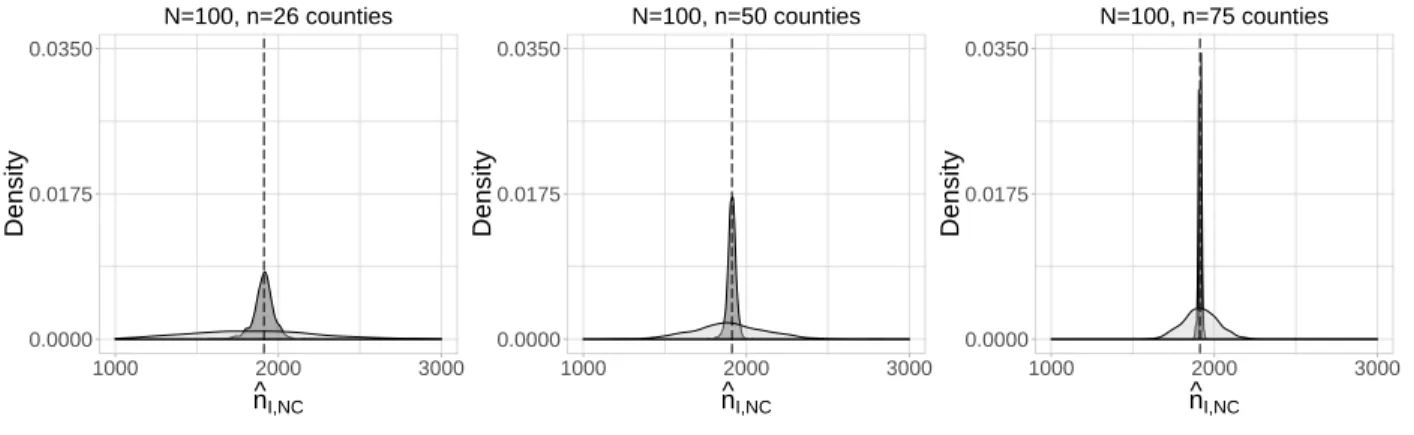
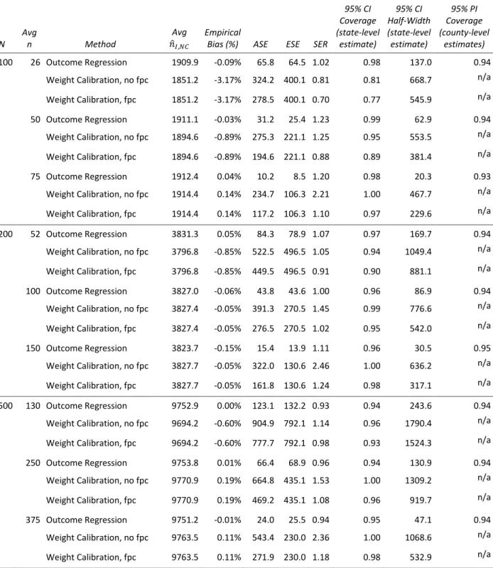
The simulation results are summarized in Table 2.1 for each of the nine finite population size by sample size combinations. Density plots for the distribution ofˆnI,N C,ORandˆnI,N C,W C across the R= 1000simulated datasets forN = 100are shown in Figure 2.2. Density plots for theN = 200

(41)

sample sizes, the distributions of both estimators are centered close to the true value of nI,N C (depicted with vertical dotted lines in Figure 2.2).

For outcome regression, the average estimated standard error tracked fairly closely with the empirical standard error. The outcome regression confidence intervals were slightly conservative for the smallest finite populationN = 100, but but the empirical coverage was close to the nominal 95% for the larger finite populations. The weight calibration method exhibited undercoverage when N = 100,n = 26, regardless of whether or not the finite population correction (fpc) adjustment was made. The observed coverage rates were 77% and 81% with and without the fpc, respectively. For larger finite population sizes, weight calibration tended to be conservative when the fpc was ignored and provided close to nominal coverage when the fpc was applied.

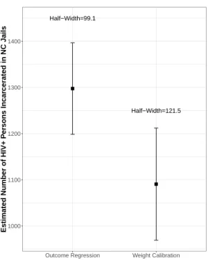
The outcome regression method led to more precise estimates ofnI,N C, as the 95% confidence interval half-widths were much smaller than the weight calibration half-widths for all population and sample size scenarios. This is depicted in Figure 2.2, as there is more spread in the distributions of the estimates for the weight calibration method compared to the outcome regression method, regardless of the population size or the sample size. County-level prediction intervals for the outcome regression approach had the appropriate level of coverage of the true values, as 94-95% of prediction intervals included the truenI,iacross theR= 1000simulated samples for each scenario.

(42)

0.0000 0.0175 0.0350

1000 2000 3000 n^I,NC

Density

N=100, n=26 counties

0.0000 0.0175 0.0350

1000 2000 3000 n^I,NC

Density

0.0000 0.0175 0.0350

1000 2000 3000 n^I,NC

Density

Outcome Regression Weight Calibration

(43)

Table 2.1: Simulation Summary Results,R= 1000Simulations

N Avg

n Method

Avg

𝑛̂𝐼,𝑁𝐶

Empirical

Bias (%) ASE ESE SER

95% CI Coverage (state-level

estimate)

95% CI Half-Width (state-level estimate)

95% PI Coverage (county-level

estimates)

100 26 Outcome Regression 1909.9 -0.09% 65.8 64.5 1.02 0.98 137.0 0.94

Weight Calibration, no fpc 1851.2 -3.17% 324.2 400.1 0.81 0.81 668.7 n/a

Weight Calibration, fpc 1851.2 -3.17% 278.5 400.1 0.70 0.77 545.9 n/a

50 Outcome Regression 1911.1 -0.03% 31.2 25.4 1.23 0.99 62.9 0.94

75 Outcome Regression 1912.4 0.04% 10.2 8.5 1.20 0.98 20.3 0.93

Weight Calibration, no fpc 1914.4 0.14% 234.7 106.3 2.21 1.00 467.7 n/a

Weight Calibration, fpc 1914.4 0.14% 117.2 106.3 1.10 0.97 229.6 n/a

200 52 Outcome Regression 3831.3 0.05% 84.3 78.9 1.07 0.97 169.7 0.94

500 130 Outcome Regression 9752.9 0.00% 123.1 132.2 0.93 0.94 243.6 0.94

250 Outcome Regression 9753.8 0.01% 66.4 68.9 0.96 0.94 130.9 0.94

(44)

2.4 Preliminary Data Results

The outcome regression and weight calibration methods were implemented on the preliminary data, as outlined in Section 2.2. For both methods, annual jail admissions, daily jail populations, index crime rates, and the number of defendants per county were square-root transformed to reduce skewness of these variables and thus the over-influence of the largest counties on model fit.

2.4.1 Outcome Regression

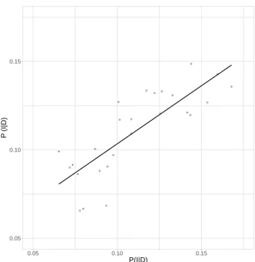
Figure 2.3 compares the knownP(I |D)_i with the estimatedPˆ(I |D)_i in the 26 counties for which the outcome regression model was fit. These values align fairly well along the 45-degree line of equality (R2 _{= 0}_.₆₅₆_{), which is indicative of reasonable model prediction. Table 2.2 displays the}

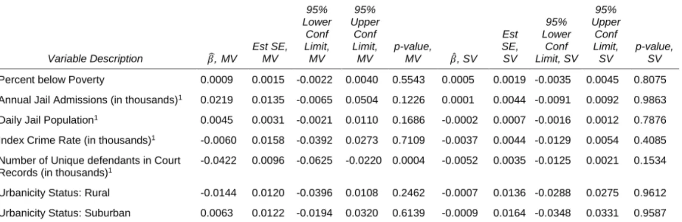
estimated model parameters. When predictingP(I |D)_i based on these covariates one at a time (single variable, or SV, models) or using all covariates simultaneously (the multivariable, or MV, model), the number of unique defendants is the strongest predictor ofP(I |D)_i. This predictor is stronger when conditioning on the other predictors than it is marginally. Because of the high correlation among the set of predictor variables, a sensitivity analysis was conducted with subsets of predictor variables to ensure robustness of the findings. The resultingnˆI,N C,ORestimates and 95% confidence intervals were similar for all models examined.

(45)

●

● ●

●

● ●

●

● ●

●

● ●

●

● ●

0.05 0.10 0.15

P(I|D)

P

^ (I|D)

Figure 2.3: Predicted vs. Actual Proportion of Defendants who were Incarcerated, n= 26Counties with Publicly-Available Jail Rosters

2.4.2 Weight Calibration

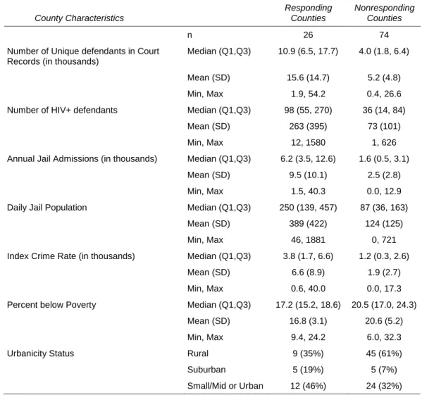
The association between county response status in the study (i.e., the availability of jail roster data) and the covariates of interest was explored. Table 2.4 presents the distribution of covariates by county response status. Responding counties tend to have more total defendants and HIV-positive defendants compared to nonresponding counties. Annual jail admissions, daily jail populations, and index crime rates are also higher in responding counties than nonresponding counties. Nonresponding counties have higher poverty rates and are more rural compared to responding counties.

(46)

Table 2.2: Parameter Estimates for Multivariable and Single Variable Prediction Models, Outcome Regression

Variable Description 𝛽,̂ MV

Est SE, MV 95% Lower Conf Limit, MV 95% Upper Conf Limit, MV p-value, MV 𝛽̂, SV

Est SE, SV 95% Lower Conf Limit, SV 95% Upper Conf Limit, SV p-value, SV

Percent below Poverty 0.0009 0.0015 -0.0022 0.0040 0.5543 0.0005 0.0019 -0.0035 0.0045 0.8075

Annual Jail Admissions (in thousands)1 _0.0219 _{0.0135 -0.0065} _0.0504 _0.1226 _0.0001 _{0.0044 -0.0091} _0.0092 _0.9863

Daily Jail Population1 _0.0045 _{0.0031 -0.0021} _0.0110 _0.1686 _-0.0002 _{0.0007 -0.0016} _0.0012 _0.7876

Index Crime Rate (in thousands)1 _-0.0060 _{0.0158 -0.0392} _0.0273 _0.7109 _-0.0037 _{0.0044 -0.0129} _0.0054 _0.4085

Number of Unique defendants in Court Records (in thousands)1

-0.0422 0.0096 -0.0625 -0.0220 0.0004 -0.0052 0.0035 -0.0125 0.0021 0.1534

Urbanicity Status: Rural -0.0144 0.0120 -0.0396 0.0108 0.2462 -0.0007 0.0136 -0.0288 0.0275 0.9612

Urbanicity Status: Suburban 0.0063 0.0122 -0.0194 0.0320 0.6139 -0.0009 0.0164 -0.0348 0.0331 0.9587

MV=Multivariable; SV=Single Variable; Est SE=Estimated Standard Error;

1_{Square-root transformed}

was excluded from the standard error calculation. The model parameters are presented in Table 2.5. County urbanicity status, the number of HIV-positive defendants, and annual jail admissions were all associated with county response status at theα= 0.1level in the multivariable calibration model.

The calibrated weights exhibited a fairly high amount of variation, ranging from1.45×10−6

to24.7(with a median of0.05). Based on the calibrated weights,nˆI,N C,W C = 1090.6, with a 95% confidence interval of(969.1,1212.1).

(47)

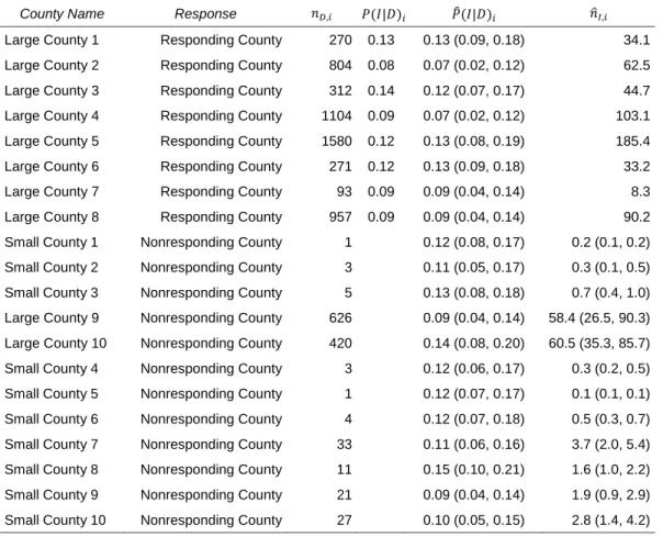
Table 2.3: Estimated Number of HIV-positive Persons Incarcerated in Jails in the 10 Largest and 10 Smallest Counties, Outcome Regression

County Name Response 𝑛𝐷,𝑖 𝑃(𝐼|𝐷)𝑖 𝑃̂(𝐼|𝐷)𝑖 𝑛̂𝐼,𝑖

Large County 1 Responding County 270 0.13 0.13 (0.09, 0.18) 34.1

Small County 1 Nonresponding County 1 0.12 (0.08, 0.17) 0.2 (0.1, 0.2)

Large County 9 Nonresponding County 626 0.09 (0.04, 0.14) 58.4 (26.5, 90.3)

Large County 10 Nonresponding County 420 0.14 (0.08, 0.20) 60.5 (35.3, 85.7)

(48)

Table 2.4: County Characteristics by Response Status

County Characteristics

Responding Counties

Nonresponding Counties

n 26 74

Number of Unique defendants in Court Records (in thousands)

Median (Q1,Q3) 10.9 (6.5, 17.7) 4.0 (1.8, 6.4)

Mean (SD) 15.6 (14.7) 5.2 (4.8)

Min, Max 1.9, 54.2 0.4, 26.6

Number of HIV+ defendants Median (Q1,Q3) 98 (55, 270) 36 (14, 84)

Mean (SD) 263 (395) 73 (101)

Min, Max 12, 1580 1, 626

Annual Jail Admissions (in thousands) Median (Q1,Q3) 6.2 (3.5, 12.6) 1.6 (0.5, 3.1)

Mean (SD) 9.5 (10.1) 2.5 (2.8)

Min, Max 1.5, 40.3 0.0, 12.9

Daily Jail Population Median (Q1,Q3) 250 (139, 457) 87 (36, 163)

Mean (SD) 389 (422) 124 (125)

Min, Max 46, 1881 0, 721

Index Crime Rate (in thousands) Median (Q1,Q3) 3.8 (1.7, 6.6) 1.2 (0.3, 2.6)

Mean (SD) 6.6 (8.9) 1.9 (2.7)

Min, Max 0.6, 40.0 0.0, 17.3

Percent below Poverty Median (Q1,Q3) 17.2 (15.2, 18.6) 20.5 (17.0, 24.3)

Mean (SD) 16.8 (3.1) 20.6 (5.2)

Min, Max 9.4, 24.2 6.0, 32.3

Urbanicity Status Rural 9 (35%) 45 (61%)

Suburban 5 (19%) 5 (7%)

(49)

Table 2.5: Parameter Estimates for Weight Calibration Model

Variable Description 𝛾̂ Est SE

95% Lower Conf Limit

95% Upper Conf Limit

P-Value

Intercept 23.062 10.696 1.84 44.28 0.0335

Urbanicity Status: Rural or Suburban1 _-6.908 _3.504 _-13.86 _{0.04 0.0514}

Number of Unique defendants in Court Records (in thousands)2

-2.097 1.308 -4.69 0.50 0.1121

Number of HIV-positive Defendants 0.029 0.015 -0.00 0.06 0.0557

Annual Jail Admissions (in thousands) 2 _-7.648 _3.386 _-14.37 _{-0.93 0.0261}

Index Crime Rate (in thousands) 2 _-0.806 _2.036 _-4.84 _{3.23 0.6930}

Percent below Poverty -0.009 0.151 -0.31 0.29 0.9523

1_{Small/Midsize, Urban is the reference level} 2_{Square-root transformed}

Half−Width=99.1

Half−Width=121.5

1000 1100 1200 1300 1400

Outcome Regression Weight Calibration

Estimated Number of HIV+ P

er

sons Incar

cerated in NC Jails

(50)

2.5 Discussion

Record linkage across three large NC databases, combined with outcome regression or weight calibration, will allow for indirect estimation of a rare population that cannot be directly measured given the current data collection practices and capabilities of NC jails. There are advantages and limitations of each method that are specific to the application at hand. Outcome regression has the advantage of producing county-level estimates, which will be useful for practitioners for targeting HIV interventions where they are most needed. However, outcome regression approaches rely on correct outcome model specification (Hansen, 1987). Weight calibration can be used to obtain an overall estimate for the entire state of NC, and the available covariates were predictive of county-level response status. The weight calibration model is doubly robust, providing consistent estimates if either the outcome model or the implied response model is correctly specified, but it unfortunately cannot provide county-level estimates. Furthermore, findings from the simulation called into question the small sample properties of its variance estimator for this population. In the simulations, the fpc was applied to the calibration model variance estimator without a formal justification. Use of the fpc led to more appropriate confidence interval coverage compared to ignoring the fpc adjustment for larger finite populations.