Technology Upgrading in Imperfectly Competitive Markets
Ryan C. Burk
A dissertation submitted to the faculty of the University of North Carolina at Chapel Hill in partial fulfillment of the requirements for the degree of Doctor of Philosophy in the Department of Economics.
Chapel Hill 2013
Approved by:
Dr. Brian McManus
Dr. Gary Biglaiser
Dr. Donna Gilleskie
Dr. Peter Norman
c
2013
Abstract
RYAN C. BURK: Technology Upgrading in Imperfectly Competitive Markets (Under the direction of Dr. Brian McManus)
Technological advancement is an inherently dynamic process. Yet, existing technology
adoption models in both the theoretical and empirical economics literatures focus on firms’
reaction to a single new technology. This research aims to extend both strands of the literature
by examining how the prospect of future technological advancement alters firms’ incentives to
adopt new technologies in the presence of spillover effects. First, in joint work with Dr. Tim
Moore, we extend the theoretical literature by introducing a second cost-reducing technology
to the seminal duopoly technology adoption timing game. Through a variety of simulations
we examine how the rate of technological diffusion and total market welfare are affected by
the second advancement. We show that the presence of an additional advancement generally
seems to decrease the overall inefficiency in a duopoly market. Second, I solve and estimate an
innovative model where competing firms make repeated decisions regarding whether or not to
upgrade their technology. Each firm’s choice directly affects the incentives of its competitors
as the technological frontier progresses. Firms face uncertainty regarding the release of future
advancements and optimize accordingly. Not surprisingly, adding technological advancements
to the standard model changes firms’ equilibrium adoption dates of the first technology.
Con-ditional on the parameterization of the model there exists a unique equilibrium outcome of the
dynamic upgrading game. However, different parameterizations can generate a variety of firm
behaviors. Using a novel dataset I estimate the model in the context of hospitals’ replacement
of MRI equipment. Results suggest that there are a complicated collection of effects that
Acknowledgments
I owe thanks to a number of people for their help through this entire process. Lindsay, while
I am sure you thought the end would never be reached, your constant support has been
indispensable along the way. The same is true for the rest of my family, Karen, Steve, and
Kelley, as well as Ron and Izzy. I would like to thank my dissertation advisor, Brian McManus,
who graciously took the time to answer all of my thousands of questions from the start. I would
also like to thank Gary Biglaiser, Donna Gilleskie, Peter Norman, and Helen Tauchen for their
helpful input and recommendations. I am also deeply indebted to Jane Darter and Randy
Randolph at The Cecil G. Sheps Center for supplying portions of my dataset. Finally, I would
Table of Contents
List of Tables . . . vii
List of Figures . . . ix
1 Introduction . . . 1
2 To Adopt or Not? A Duopoly Model of Technology Upgrading . . . 3
2.1 Introduction . . . 3
2.2 Model . . . 7
2.2.1 Pareto Efficiency . . . 11
2.2.2 Monopoly . . . 15
2.2.3 Cournot Competition . . . 17
2.3 Simulations . . . 28
2.4 Conclusion . . . 37
3 Technology Upgrading in Imperfectly Competitive Markets: The Case of MRI . . . 38
3.1 Introduction . . . 38
3.1.1 Related Literature . . . 41
3.2 Model . . . 45
3.2.1 Static Pricing Game . . . 46
3.2.2 Dynamic Technology Adoption Game . . . 48
3.2.3 Backwards-Induction Algorithm . . . 54
3.3 Data . . . 66
3.3.1 The Market for MRI . . . 66
3.3.2 Data Collection and Sample Selection . . . 68
3.4 Estimation . . . 75
3.4.1 Descriptive Results . . . 75
3.4.2 Empirical Model . . . 80
3.5 Conclusion . . . 86
A Chapter 2 Appendices . . . 88
A.1 Tables and Figures . . . 88
A.2 Bertrand Stage Game . . . 105
A.3 Issues with Discrete Time . . . 109
B Chapter 3 Appendices . . . 112
B.1 Simulation Results . . . 112
B.2 Data Collection . . . 125
B.3 Sample Statistics . . . 129
B.4 Descriptive Results . . . 134
B.5 Results . . . 141
List of Tables
3.1 Base Parameterization . . . 62
3.2 Variables Collected Through State CON Programs . . . 71
A.1 Continuation Values in Figure A.6 wheren=t−T . . . 88
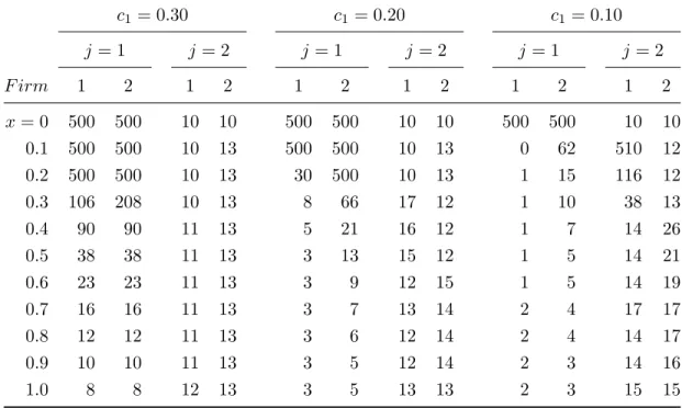
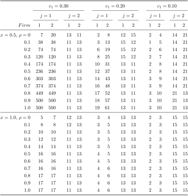
A.2 Duopoly Adoption Dates for Different Parameterizations ofC(n) . . . 89
A.3 Duopoly Adoption Dates for Different Firm Beliefs (ρ) . . . 90
A.4 Monopoly, Duopoly, and Efficient Adoption Dates for Different Marginal Cost Vectors and Adoption Costs . . . 91
A.5 Duopoly and Socially Optimal Adoption Dates and Total Surplus for Different Beliefs (ρ) . . . 92
B.1 Simulation Flow Profit Levels Using the Base Parameterization . . . 115
B.2 1,000 Simulations with Homogeneous Firms (by order ofmoves) . . . 116
B.3 1,000 Simulations with Homogeneous Firms (by order ofadoption) . . . 117
B.4 1,000 Simulations with Heterogeneous Firms (by order of moves) . . . 118
B.5 1,000 Simulations with Heterogeneous Firms (by order of adoption) . . . 119
B.6 1,000 Simulations with Homogeneous Firms (by order ofmoves) . . . 120
B.7 1,000 Simulations with Homogeneous Firms (by order ofadoption) . . . 121
B.8 1,000 Simulations with Heterogeneous Firms (by order of moves) . . . 122
B.9 1,000 Simulations with Heterogeneous Firms (by order of adoption) . . . 123
B.10 1,000 Simulations with Asymmetric Firms (by order of moves) . . . 124
B.11 Hospital- and Market-Level Sample Statistics (with corresponding values for the contiguous US) . . . 132
B.12 Years Until First Adoption for Each Hospital By Market Size . . . 133
B.14 Multinomial Logit Regression Results of Initial Adoption Date Versus Hospital-and Market-Level Covariates (Base Outcome: Initial Adoption in 1983–1992) . 135
B.15 Proportional Hazard Model of Initial Adoption Date with Hospital- and Market-Level Covariates (Using a Weibull Distribution) . . . 136
B.16 Ordered Probit Regressions of Hospital-Level Technology Entering 2008 Versus Hospital- and Market-Level Covariates (For Different Release Dates of the New Technologies) . . . 137
B.17 Ordered Probit Regressions of Hospital-Level Technology Entering 2008 Versus Hospital- and Market-Level Covariates (For Different Release Dates of the New Technologies) . . . 138
B.18 Proportional Hazard Model ofθ=N Adoption Date with Hospital- and Market-Level Covariates (Using a Weibull Distribution) . . . 139
B.19 Proportional Hazard Model ofθ=N Adoption Date with Hospital- and Market-Level Covariates (Using a Weibull Distribution) . . . 140
B.20 Parameter Estimates for the Model Assuming Every Hospital is a Monopolist 141
B.21 Parameter Estimates for the Two-Technology Model . . . 142
B.22 Parameter Estimates for the Two-Technology Model . . . 143
List of Figures
3.1 Calculating Expected Continuation Values in TN −1 . . . 59
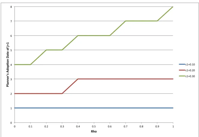
A.1 Planner’s Adoption Date of j = 1 for Different Values of ρ and c1 (where c0 = 0.4,β = 0.9, andC(n) = 1/(1 +n)) . . . 92
A.2 Efficient and Monopoly Adoption Dates for j=2 (where β = 0.9 and C(n) = 1/(1 +n)) . . . 93
A.3 Monopoly Adoption Dates for j=1 (β = 0.9, p= 0.1) . . . 94
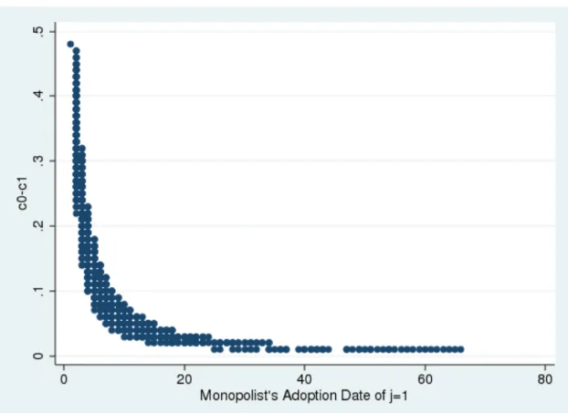
A.4 Scatter Plot ofc0−c1 versus Monopoly Adoption Dates for j=1 . . . 95
A.5 Cournot Adoption Dates forj = 2 in States (T,0, a, a) . . . 96
A.6 Example Continuation Game Beginning in State (T,0,1,0) where (β = 0.9, c0 = 0.35, c1= 0.15) . . . 97
A.7 Cournot Adoption Dates (# of Periods AfterT) in State (T,0,1,0) . . . 98
A.8 Total Monopoly Inefficiency, Including Adoption Costs (whereC(n) = (1+1n)x) . 99 A.9 Total Duopoly Inefficiency, Including Adoption Costs (whereC(n) = (1+1n)x) . 100 A.10 Difference in Total Intertemporal Surplus (Duopoly – Monopoly), Including Adoption Costs (where C(n) = (1+1n)x) . . . 101
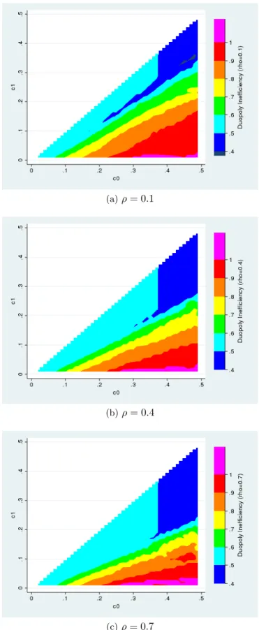
A.11 Total Duopoly Inefficiency, Including Adoption Costs for Different Values ofρ (where C(n) = (1+1n)0.5) . . . 102
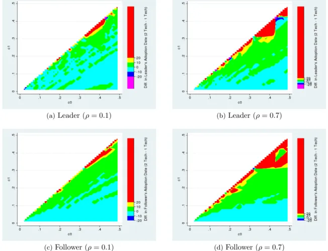
A.12 Difference in Adoption Dates of j = 1 for a Two- vs. One-Technology Model (Two-Technology Date – One-Technology Date, Color Scale Maintained Through-out) . . . 103
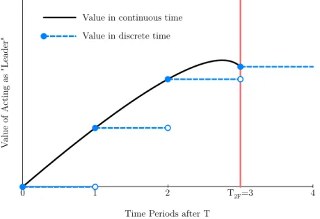
A.13 Difference in Total Inefficiency (One-Technology Model – Two-Technology Model)104 A.14 A Situation where a Diffusion Equilibrium in Continuous Time Appears to be a Joint-Adoption Equilibrium in Discrete Time . . . 109
A.15 Discrete Time Preemption Does Not Lead to Equal Continuation Values . . . 110
B.1 Cumulative Probability ofθ= 1 Uptake for Different (J, N) Pairs . . . 112
B.3 Average Adoption Date ofθ= 1 for Different Values ofx, whereC(t) = 10/(1 +
t)x/10 (J = 2, N = 2) . . . 114
B.4 Sample Market Size Distribution . . . 129
B.5 Total Number of MRI Scanners Purchased in Each Year . . . 130
B.6 Median Adoption Cost in Each Year . . . 130
B.7 Kaplan-Meier Failure Function By Market Size . . . 131
B.8 Total Number of Initial Adoptions by Year . . . 131
Chapter 1
Introduction
Technologies are constantly evolving in every sector of the economy. As new advancements
are released firms are forced to make repeated decisions regarding whether or not to upgrade
their existing technology. In imperfectly competitive markets this decision process is
compli-cated by the fact that each firm’s choice has spillover effects on its competitors. However,
there is currently a void in both the theoretical and empirical economics literatures merging
the analysis of these two ideas. My research attempts to fill this gap by examining strategic
interactions between firms while striving to better capture the dynamics inherent in
techno-logical innovation. In general I find that adding multiple waves of technotechno-logical advancements
to the standard one-technology models can cause firms’ adoption incentives to vary
signifi-cantly. In fact, equilibrium adoption dates in one-technology models are typically suboptimal
in a multiple-technology context. As a result, any policy prescription derived from a
single-technology model is likely flawed if firms are making dynamic single-technology upgrading decisions.
In the second chapter of this dissertation my co-author, Tim Moore, and I extend the
seminal duopoly technology adoption model in the theoretical literature to include a second
technology. Despite this seemingly straightforward extension we find that the equilibrium
analysis quickly becomes complicated. We circumvent this issue by running a variety of
sim-ulations and comparative statics exercises aimed at examining the equilibrium properties of
the model. We find that overall market inefficiency seems to decrease with the addition of a
second technological advancement despite the additional adoption costs. Further, we find that
The third chapter of this dissertation examines a more general technology adoption game
that allows for more than two firms and technologies. The key difference between the two
models is that here I assume firms make technology adoption decisions sequentially in order to
make the solution tractable. Despite this difference the theoretical results from the two models
are qualitatively very similar. In addition to the theoretical results I also estimate the model
using a novel dataset that tracks hospitals’ purchases of magnetic resonance imaging (MRI)
equipment over a 28-year period. I find that adoption decisions are a complicated function
of both hospital- and market-level variables. Extending the empirical framework to include
multiple technologies poses significant data, computing, and modeling issues. However, the
Chapter 2
To Adopt or Not? A Duopoly Model of Technology Upgrading
2.1 Introduction
Dating back to the seminal works by Reinganum (1981b) and Fudenberg and Tirole (1985),
a significant strand of the theoretical literature has focused on technology adoption timing
games. In both models a dynamic game begins when a technological innovation is released to
a duopoly market. Each firm’s strategy involves choosing a single point in time to adopt the
new technology. As time passes the cost of adopting the technology decreases, generating a
tradeoff between adopting sooner at a higher cost (and potentially inducing one’s competitor
to delay adoption) versus waiting to adopt at a lower cost. Reinganum (1981b) shows that
even though firms are ex ante identical, in any precommitment (Nash) equilibrium, the two
firms adopt at different points in time, leading to a “diffusion” of the technology. Fudenberg
and Tirole (1985) show that in the Reinganum (1981b) precommitment equilibrium the firm
that commits to adopting first earns higher profits at its competitor’s expense. Further, they
examine subgame perfect Nash equilibria which enables each firm to preempt its competitor.
They show that this preemption incentive drives the “follower” in the Reinganum (1981b)
equilibrium to preempt the “leader.” Each firm continues to preempt its competitor until it is
no longer profitable and both firms’ payoffs are equalized.1 Fudenberg and Tirole (1985) also
demonstrate that for certain parameterizations of the model late “joint” adoption equilibria
1The follower’s adoption date is the same in both the Nash and subgame perfect Nash equilibria
may exist in addition to the diffusion equilibrium.
A variety of papers have extended these seminal models in several directions. For example,
in a model with asymmetric firms Riordan (1992) examines how price and entry regulations
can affect technological diffusion. He finds that regulations can limit each firm’s incentive to
preempt its competitor and slow the diffusion of the new technology. There is no uncertainty
regarding a technology’s value and that value is realized immediately upon adoption. Other
models, such as Hoppe (2000) and related papers, incorporate a learning process regarding the
new technology’s profitability. Stenbacka and Tombak (1994) examine uncertainty regarding
the amount of time needed to successfully implement a new technology. There are also a
number of duopoly models focused on situations where waiting to adopt rather than preempting
can be advantageous. Three such examples are Katz and Shapiro (1987), Dutta, Lach, and
Rustichini (1995), and Hoppe and Lehmann-Grube (2005).2
All of the aforementioned models involve asingle new technology. However, we argue that
most technological innovations are subsequently updated and improved. Newer advancements
allow firms to operate more efficiently by improving productivity, decreasing costs, enhancing
communication and connectivity, and providing firms with more detailed information about
consumers’ preferences. As a result, while a firm decides whether or not to adopt a new
technology today, the technological frontier is advancing. Thus, a firm’s purchasing decision
implicitly incorporates expectations about the likelihood and potential benefit of future
ad-vancements. As time passes and newer technologies are released, firms must make repeated
decisions regarding when/whether toupgrade their current technology. Yet, the current
litera-ture largely abstracts from these dynamic considerations. Two notable exceptions are Horner
(2004) and Harrington, Iskhakov, Rust, and Schjerning (2010).3 Horner (2004) models R&D
competition between two firms as an endless race. In each period the two firms choose a costly
2For a somewhat recent review of the literature see Hoppe (2002).
3While Huisman and Kort (1999) and Huisman and Kort (2000) also analyze multi-technology
effort level that affects the probability of generating a successful innovation. He finds that
in-vestment efforts increase when the firms’ technologies are further apart which contradicts the
typical intuition in the R&D literature. In a working paper, Harrington, Iskhakov, Rust, and
Schjerning (2010) also develop a dynamic duopoly model where firms can make investments in
order to decrease their marginal cost of production. In each period the duopolists
simultane-ously decide whether or not to adopt a new technology that evolves according to a first-order
Markov process. Once the technology choices are made profits are determined through a static
Bertrand pricing game. While simultaneous adoption cannot be an equilibrium in a static
version of the game, the authors show that investment does occur in the dynamic game.4
Fur-ther, the authors show that a wide range of equilibria existfor a given parameterization of the
model. Some equilibria exhibit “leap-frogging” where one firm invests in a new technology and
undercuts its rival’s price. The firm at a cost disadvantage may then subsequently undercut
its rival when an improved technology is released. Other equilibria involve “sniping” where
one firm builds a large cost advantage over time until the competitor invests and undercuts
its rival. Additionally, equilibria exist where only one of the two firms ever adopts new
tech-nologies. However, certain aspects of the model are somewhat unclear. For one, the authors
state that most of the “interesting” equilibria occur when firms are “asymmetric” in the sense
that the firm indices matter but do not clarify the source of this asymmetry.5 Second, the
authors state that they use an equilibrium selection rule that in essence forces firms to engage
in leap-frogging behavior but then illustrate “non-leap-frogging” equilibria in their simulation
results. Despite these ambiguities it is clear that a simple extension to the static Bertrand
4Consider the standard static Bertrand pricing game except that each firm has the ability to invest
in a marginal cost-reducing technology. It is unprofitable if both firms adopt the technology because equilibrium profits are driven to zero (and the firms pay a fixed cost associated with the investment). The authors define this situation as the “Bertrand Investment Paradox” and show that it does not hold in a dynamic setting.
5In the paper the authors essentially discuss two different models. In a complete information setting
pricing game can generate a wide range of equilibrium investment and price paths. The model
we propose is qualitatively similar to the Harrington, Iskhakov, Rust, and Schjerning (2010)
model except for a key difference. In their model the cost of adopting each new technology is
time-invariant. In other words, the cost of adopting the best technology today is the same as
it would be tomorrow so long as an even newer technology is not released.6 Given that costs
are constant and the probability that a new technology is released follows a first-order Markov
process, there is no incentive for a follower to wait to adopt the best technology available.
Thus, technological diffusion is “degenerate” in the sense that a given technology does not
diffuse gradually through time.7
We take a different approach and extend the model of Fudenberg and Tirole (1985) by
introducing a second technology. There is objective uncertainty regarding the release of the
second advancement but not its affect on each firm’s profitability. We assume that the firms
are Cournot competitors and choose quantities myopically in each period.8 The cost of
adopt-6Giovannetti (2001) develops a similar model where the evolution of the best technology is
exoge-nous. Specifically, an improved technology (i.e. a lower marginal cost of production) only becomes available if a firm adopts the existing technology. Again, the cost of adopting a given technology is constant over time.
7It is somewhat unclear if it can ever be an equilibrium for both firms to adopt a new technology
immediately when it is released if firms employ pure strategies. Joint adoption in a static version of the game cannot be an equilibrium because each firm has an incentive to deviate. However, in a dynamic setting it is hypothetically possible for both firms to adopt simultaneously in an attempt to transition to a better future state. In all of the simulated equilibria developed in the paper this outcome never occurs.
8Two papers use Cournot demand to examine how market concentration affects adoption dates
ing each technology declines as time passes since its release. Our goal is to examine how the
rate of technological diffusion is altered when firms are faced with the prospect of a future
advancement. We find that the addition of a second technology greatly complicates the
equi-librium analysis. In general, very little can be said about the equiequi-librium properties of the
entire dynamic game. This issue arises primarily from the fact that it is difficult to rank the
firms’ continuation values before the second technology is released. Since we cannot derive
many results in general, we instead run a number of simulations aimed at illustrating the
equilibrium properties of the model. Further, we solve for the monopoly and socially optimal
outcomes of the game and use them as a benchmark against the duopoly game. Finally, we
show that if firms instead compete in prices and time periods are “short enough,” at most
one of the two firms will ever adopt the new technologies. This result seems to contradict the
leap-frogging behavior discussed in Harrington, Iskhakov, Rust, and Schjerning (2010).
The remainder of the paper is organized as follows. Section 2 develops the model and
the solutions for the socially optimal, monopoly, and duopoly cases. Section 3 discusses the
simulation results and Section 4 concludes. Appendix A.1 contains all of the figures and tables.
Appendix A.2 solves for the equilibrium assuming that a Bertrand rather than Cournot stage
game is played in each period. Finally, Appendix A.3 elaborates on several issues caused by
the use of discrete time.
2.2 Model
Consider a dynamic technology adoption game between two ex-ante identical firms. Time is
discrete and indexed by t = 0,1,2, . . . ,∞. Each period unfolds in two stages. In the first stage the two firms (indexed by i= 1,2) simultaneously decide whether or not to adopt the most efficient technology available. Technologies are indexed by j = 0,1,2. It is assumed that both firms enter periodt= 0 operating with technology j= 0 (the “original” or “status quo” technology). A technological advancement, j = 1, is released at the beginning of t= 0.
Technology j = 1 is the most efficient technology available until j = 2 is released at the beginning of an unknown date in the future,T, where we assume 0< T <∞. In each period 0 < t < T, both firms believe that a new technology will be released at the beginning of the next period with probability ρ.9 For simplicity, we assume that once j = 2 is released,j = 1 can no longer be purchased by a firm operating with technologyj = 0.
Given the technological choices from the first stage of each period, the firms subsequently
engage in a static Cournot game to determine output and flow profit levels. The game involves
perfect monitoring so that once the technology choices are made they are common knowledge.10
Letati ∈Ati denote firmi’s action in the first stage of period t, chosen from the set of feasible actions available to the firm in that period, where
Ati =
{0,1} ift= 0
{0,1} ifati−1 = 0 and 0< t < T {1} ifati−1 = 1 and 0< t < T {0,2} ifati−1 = 0 and t≥T {1,2} ifati−1 = 1 and t≥T {2} ifati−1 = 2 and t≥T
.
Thus, we prohibit the firms from downgrading their technology.11 In each period the firms
face the following market demand function:
D(Q) = 1−Q,
where Q=q1+q2 denotes market output. Adopting a new technology affords a firm with a
decreased marginal cost. Conditional on a firm’s technology, marginal cost is assumed to be
constant. We assume that the firm’s marginal cost associated with technology j,cj, satisfies
9For now firms do not update their beliefs regarding the release of the second technology. 10Strictly speaking, the game is one of perfect monitoring bothwithin andbetween periods.
11Neither firm would ever find it optimal to downgrade its technology because the fixed cost of
the following:
1
2 > c0> c1> c2= 0.
The upper bound of 1/2 is imposed to prevent a firm from finding it optimal to produce zero
in any period. Suppressing the time superscript, letπ(ai, a−i) denote firm i’s flow profit in a period where it chooses technology ai and its competitor chooses technology a−i. Given the assumption of Cournot competition, qi andπ(ai, a−i) satisfy the following:
qi=
1−2cai+ca−i 3
π(ai, a−i) =qi2,
where flow profits are assumed to be time-invariant and the scrap value of a firm’s old
tech-nology is taken to be negligible.12
The cost of adopting the most recent technology n periods after its release is denoted by C(n). We assume that cost function is strictly positive, strictly decreasing, and strictly convex. Although we assume that both technologies follow the same cost schedule it is straightforward
to allow the function to vary by technology (as long as it satisfies the aforementioned properties
and all functional forms are common knowledge at the beginning of the game).
Let a state s∈S be a quadruple (t, n, ati−1, at−−i1), wheretdenotes the current time period, n denotes the number of time periods since the release of the most recent technology, ati−1 denotes firmi’s technology choice in the previous period, andat−−i1 denotes firmi’s competitor’s technology choice in the previous period. Note that if t > n it must be that t ≥ T and the second technology,j = 2, has been released. Given the definition of a state, firm i’s Bellman
12Imposing a specific functional form onπ(·) represents a departure from the setup in Fudenberg and
equation can be written as
Vi(t, n, ati−1, at
−1
−i ) = max at
i∈Ati
π(ati, at−i)−1[at i6=a
t−1
i ]C(n)+ β
ρV(t+ 1,0, ati, at−i) + (1−ρ)V(t+ 1, n+ 1, ati, at−i)
, (2.1)
whereρ= 0 for all t≥T.
Since there are a finite number of technologies, the equilibrium analysis employs backwards
induction. First, the continuation game beginning in period T is analyzed. The equilibrium outcome(s) from this game form the continuation values for all periodst < T when the uncer-tainty has yet to be resolved. Given these values each firm’s optimal strategy is characterized
for all states where t < T. At this point it is instructive to informally discuss firms’ strate-gies and the equilibrium concept that we employ.13 First, for simplicity we focus exclusively
on pure-strategy equilibria even though mixed-strategy equilibria also exist. Additionally, we
focus on a very specific type of Markov perfect equilibrium where the firms’ output choices in
each period are static. As a result, we abstract from situations where firms could use
pun-ishment strategies to enforce a (potentially) Pareto-improving equilibrium. Thus, conditional
on the vector of technology choices in the period, firms’ outputs and profits are trivial. While
we solve for the Markov perfect equilibria of the game, it is somewhat unconventional for a
Markov state to be a function of the time period. Here, the Markov state is dependent on the
number of periods that have elapsed since the release of the best technology available. Since
C(n) is strictly decreasing in n and flow profits are not linear in technologies, no two states in the game are the same.14 Therefore, we cannot group states into equivalence classes and
solve for the firms’ optimal strategies in each set of states. We use the term “Markov” because
the actual dates of earlier adoptions are irrelevant to the firm’s optimization problem in the
13We choose to avoid developing unnecessary notation because we do not subsequently use it at any
other point in the paper.
14The only exceptions are states (t, t,1,1) and (t, n,2,2). In (t, t,1,1), where t < T, both firms have
current period. Put differently, it only matterswhether or not a firm has adopted a technology,
notwhen the adoption occurred. Before analyzing the duopoly game, we characterize both the
Pareto optimal and monopoly outcomes. Both situations are used as benchmarks for
compari-son against the duopoly outcome. It is difficult (especially in the duopoly case) to prove results
in general. Therefore, we often refer to specific examples in order to illustrate tradeoffs and
equilibrium properties of the model. Unless otherwise noted, the reader should assume that
we employ the following parameterization: β= 0.9,ρ= 0.1, T = 10, andC(n) = 1/(1 +n).
2.2.1 Pareto Efficiency
As a benchmark, consider the Pareto optimal outcome of the dynamic game. In order to
maximize total surplus it is optimal for the social planner to shutdown one of the two firms
and set the market price equal to the marginal cost of the remaining firm. Removing the
second firm eliminates all redundant adoptions of the new technologies, thereby limiting overall
adoption costs in the market.15 We assume that the planner raises revenue to pay for a new
technology through a one-time, lump-sum tax. All of the notation from the previous section
holds except that a state is now only a function of the single operating firm’s technology.
Therefore, let a states∈S be a triple (t, n, at−1), wheretandnare unchanged andat−1 is the operating firm’s action in the previous period. Let σ(a) denote the total flow surplus in the market when the planner chooses technology a. Conditional on the technology choice, total surplus in the market is given by
σ(a) = 1
2(1−ca)
2.
In all states where n < t (i.e. states where the second technology has been released) the planner faces a simple optimal stopping problem. The optimal strategy entails delaying the
adoption of technology j= 2 until the first period where the value of adopting in the current period exceeds the value of postponing adoption until the subsequent period. In any period
15Here we are implicitly assuming that there are no capacity constraints so that a single firm can
t≥T, wheren=t−T, the value of adopting j= 2 in the current period is given by
σ(2)−C(n) + β
1−βσ(2), (2.2)
and the value of delaying adoption until the subsequent period is
σ(at−1) +β
σ(2)−C(n+ 1) + β 1−βσ(2)
. (2.3)
Due to the strict convexity ofC(n), the first period where (2.2) exceeds (2.3) is the first period twhere the following inequality holds:
σ(2)−σ(at−1)> C(n)−βC(n+ 1). (2.4)
The LHS of (2.4) is the marginal increase in surplus from adopting technology j = 2 while the RHS denotes the discounted cost savings from delaying adoption by a period. As a result,
(2.4) states that the planner’s optimal policy rule is to adopt j = 2 in the first period where the benefit from adopting today (an immediate increase in surplus) exceeds the benefit from
delaying adoption until tomorrow (a decrease in the cost of j = 2). Note that since σ(a) is increasing in a, the planner adopts j = 2 weakly earlier when she enters period T with technology j= 0 than when she enters with technologyj= 1.16
In all periods t < T, the planner’s Bellman equation can be written as follows:
V(t, n,0) = max at∈{0,1} σ(a
t)−1[
at=1]C(n) +β[ρV(T,0, at) + (1−ρ)V(t+ 1, n+ 1, at)], (2.5)
where the value of having already adopted j= 1 is
V(t, n,1) =σ(1) +β[ρV(T,0,1) + (1−ρ)V(t+ 1, n+ 1,1)]. (2.6)
16At first glance it might appear that we should claim the planner adopts “strictly earlier” rather
than “weakly earlier.” In continuous time this logic is correct. However, in discrete time if c0 andc1
The planner’s optimal strategy is to delay adoption of j = 1 until the first period where the value of adopting in the current period,
σ(1)−C(n) +β[ρV(T,0,1) + (1−ρ)V(t+ 1, n+ 1,1)],
exceeds the value of delaying adoption until the subsequent period,
σ(0) +β{ρV(T,0,0) + (1−ρ)
σ(1)−C(n+ 1) +β ρV(T,0,1) + (1−ρ)V(t+ 2, n+ 2,1)
}.
Noting thatV(t+ 1, n+ 1,1) =V(t+ 2, n+ 2,1) becauseρis stationary, after simplification the planner adopts j= 1 in the first period n (where here nand t are equivalent becauset < T) when the following condition holds:
σ(1)−σ(0) +βρ[V(T,0,1)−V(T,0,0)]> C(n)−β(1−ρ)C(n+ 1). (2.7)
Again, the LHS of (2.7) is the marginal benefit of adopting in the current period. By adopting
today the planner not only increases flow surplus, but also with probabilityρshe assures herself of transitioning to a more valuable state tomorrow.17 The RHS of (2.7) is the expected cost
savings from delaying adoption until the subsequent period. So, once again, the planner delays
adoption ofj = 1 until the first period when the marginal benefit from adopting exceeds the marginal benefit from further delay. Comparing (2.7) with the corresponding condition in a
one-technology model:
σ(1)−σ(0)> C(n)−βC(n+ 1), (2.8)
it is clear that the RHS of (2.7) is weakly greater than the RHS of (2.8). In waiting to adopt
17The proof thatV(T,0,1)> V(T,0,0) is forthcoming. A sketch of the proof is as follows: (2c−c2)/2
is increasing in c for all 0 ≤ c < 0.5. So, the planner entering period T with technology 0 adopts technology 2 weakly earlier than she would if she entered periodTwith technology 1. Abusing notation, letT0denote the period when a planner entering periodT withj= 0 optimally chooses to adoptj= 2
and defineT1similarly for thej= 1 case. We know thatT0≤T1. However, thej= 1 planner could just
as easily choose T1 =T0. Thus, the decreased cost of adoption must outweigh the lower flow surplus
level (σ(1) vs. σ(2)) in all periodsT0≤t < T1. This, coupled with the fact that thej = 1 planner is
attaining a strictly higher flow surplus than thej = 0 planner in all periods T ≤t < T0 ensures that
j = 1 the planner faces a risk in the two-technology game that does not exist in the single-technology game–with probability (1−ρ) an even better technology is released and the option of adopting j= 1 no longer exists. Fixing the LHS of both (2.7) and (2.8), in any tthe cost savings threshold that must be eclipsed to induce adoption in the two-technology game is larger
(relative to the one-technology game) to compensate for this risk. As ρ approaches zero the planner’s perceived risk falls and her optimal stopping criterions in the one- and two-technology
games converge. If ρ approaches one the planner believes that there is no cost benefit from waiting (because in all t < T she believes j = 2 will be released in the subsequent period with probability one). As a result, in this case the RHS of (2.7) is simply the current cost of
adoption. While the RHS of (2.7) is larger than the RHS of (2.8), the LHS is larger as well.
As a result, the net effect of the presence ofj= 2 on the adoption date ofj= 1 is ambiguous (relative to the situation where there is only one technology). Figure A.1 illustrates the effect
of a second technology on the planner’s adoption date ofj= 1 for different values ofρand c1.
Whenρ= 0 the planner’s decision problem is equivalent in the one- and two-technology games. Therefore, whenc1 = 0.1, 0.2, and 0.3, in a one-technology model the planner adoptsj= 1 in
t= 1, 2, and 4, respectively. Whenc1 = 0.1 the increase in flow surplus from adoptingj= 1 is
relatively large. Thus, the planner adoptsj = 1 quickly (in period t= 1) and this decision is unaffected byj= 2,regardless of the value ofρ. However, consider the case wherec1 = 0.3, so
the marginal increase in flow surplus is relatively small. In a one-technology game the planner
would adoptj = 1 int= 4. The addition of a second technology delays the planner’s adoption of j = 1 and this delay is increasing in ρ. Here V(T,0,1)−V(T,0,0) = 0.065, which is less than it is in the c1 = 0.1 case (0.33), so the added benefit of potentially transitioning to a
preferred state is mitigated in the current adoption decision.18 Since the benefit of adopting
j = 1 is minimal once j = 2 is released, the sunk cost of adoption must be recouped prior to period T. As ρ increases the planner believes that the window of time when she can benefit fromj = 1 shrinks and therefore she is only willing to adopt it relatively later at a lower cost.
18In this specific parameterization the planner would adoptj= 2 in the same period (T+1) regardless
of whether she entered period T withc = 0.4 orc = 0.3. So, when c1 = 0.3,V(T,0,1) only exceeds
2.2.2 Monopoly
For the sake of comparison next assume that instead of two firms, a single monopolist operates
in the market. All of the notation holds from the Pareto efficiency analysis except that the
mo-nopolist maximizes intertemporal profit rather than surplus. Letπ(a) denote the monopolist’s flow profit when choosing technologya. Conditional on his technology choice, the monopolist maximizes per-period flow profit by setting
Q= 1−ca
2 and p= 1 +ca
2 ,
so thatπ(a) =Q2.Employing similar logic to that used in the Pareto optimal case, once j= 2 is released the monopolist’s optimal strategy is to adopt j= 2 if
π(2)−π(at−1)> C(n)−βC(n+ 1) (2.9)
and choose at =at−1 otherwise. Substituting and comparing the LHS of (2.4) with the LHS of (2.9) yields the following inequality for all 0< c <1/2:
σ(2)−σ(at−1) = 2c−c
2
2 >
2c−c2
4 =π(2)−π(a t−1).
social planner and the monopolist versus marginal cost entering periodT. It is assumed that both the planner and the monopolist enter periodT with the same technology. Note that the difference in adoption times in general decreases with c. The total intertemporal inefficiency (including adoption costs) associated with the monopolist is also plotted on the same graph
and is greatest at the “extreme” values ofc. In other words, the inefficiency is greatest when j = 2 provides either a significant or very negligible cost savings over the current technology being utilized. In the former case (when cis close to 0.5), the result appears counterintuitive because if both the planner and the monopolist are using the same technology, per-period
deadweight loss is smaller as c increases. However, the fact that the planner adopts j = 2 a period before the monopolist causes the monopoly inefficiency to increase asc increases.19 In the latter case (whencis approaching zero), there is a greater lag in the monopolist’s adoption time relative to the efficient adoption date, again causing the inefficiency to increase.
The analysis of the monopolist’s problem in all periods t < T is identical to that for the social planner, substituting π(·) for σ(·). Thus, the monopolist’s optimal strategy involves adoptingj= 1 in the first period where
π(1)−π(0) +βρ[V(T,0,1)−V(T,0,0)]> C(n)−β(1−ρ)C(n+ 1). (2.10)
This inequality is analogous to (2.7) in the social planner’s problem. Again, the mere
pres-ence of a second technology which is released at an uncertain date in the future increases the
marginal benefit of adopting in the current period but requires a greater cost savings for
adop-tion to be optimal.20 Figure A.3 is a contour plot of the monopolist’s hypothetical adoption
19This explanation is admittedly somewhat muddled. Consider the range of marginal costs 0.49>
c >0.26. In this range both the monopolist’s and the planner’s optimal adoption dates (and therefore the costs of adoption) are fixed. As c falls the monopolist’s profit, the planner’s total surplus, and per-period deadweight loss all increase,if the monopolist and the planner are operating with the same marginal cost. So, if both the monopolist and the planner adopted in the same period, the black line in Figure A.2 would be increasing in this range of marginal costs. However, in periodT+ 1 the planner adoptsj= 2 while the monopolist continues operating withc. Since a lower value ofcgenerates higher total surplus in the monopoly market, the total inefficiency in period T+ 1 is smaller for smaller c’s. This effect dominates so the one-period difference in adoption dates causes the total inefficiency to fall in this range.
date ofj = 1 over the entirec0-c1 grid.21 Not surprisingly, the figure suggests that there is a
negative relationship between the adoption date and the difference betweenc0andc1 (which is
illustrated in Figure A.4). Asc0−c1 increases, the monopolist has a greater incentive to adopt
j = 1 to increase flow profits before the release of j = 2. In other words, fixing ρ, a greater value ofc0−c1 makes adoption profitable at a higher cost which in turn allows the monopolist
to adopt earlier. Additionally, since we have shown thatV(T,0,1)−V(T,0,0)>0, waiting to adopt in the current period leads to possibility of transitioning to a less-desirable state in the
subsequent period. Fixing the difference between c0 and c1, Figure A.3 also shows that the
monopolist’s equilibrium adoption date increases as both costs increase.22
2.2.3 Cournot Competition
Now consider the original specification where two firms play a static Cournot equilibrium
in the second stage of each period. Recall that in the duopoly model a state s ∈ S is a quadruple (t, n, ati−1, at−−i1), where tdenotes the current time period, ndenotes the number of time periods since the release of the most recent technology, ati−1 denotes firm i’s technology choice in the previous period, and at−−i1 denotes firm i’s competitor’s technology choice in the previous period. As a result, the two firms can enter period T in one of four states: s ∈ {(T,0,0,0),(T,0,1,1),(T,0,1,0),(T,0,0,1)}. In the first two states, the continuation game beginning in periodT is a discrete-time version of that found in Fudenberg and Tirole (1985). As noted in Fudenberg and Tirole (1985), the use of discrete rather than continuous
time generates slightly different equilibrium outcomes.23 In the latter two states, one firm
substitutingπ(·) forσ(·).
21If T is less than the optimal adoption date, the monopolist simply would not adopt j = 1 in
equilibrium.
22We think that this is being driven in part by the fact that difference between V(T,0,1) and
V(T,0,0) decreases as c1 and c0 increase (holding c0−c1 constant). For example, if the monopolist
enters period T with any 0.25 < c < 0.35 then he will adopt j = 2 in period T + 2. However, the adoption dates are more dispersed at lower values ofc(T+ 8 ifc= 0.05 versusT + 4 ifc= 0.15).
23Specifically, as noted in Fudenberg and Tirole (1985), modeling in discrete time eliminates the
enters periodT having adopted the first advancement while the competing firm is still operating with the original technology.
Equilibrium Strategies in (T,0,0,0) and (T,0,1,1)
To simplify the exposition we focus on state (T,0,0,0). The analysis in state (T,0,1,1) is
analogous. In this state, neither firm enters period T with a technological advantage so the firms’ value functions are identical. Using backwards induction, first consider the situation
where one of the firms (w.l.o.g. firm 1) has already adopted the second technology j = 2. In this case firm 2’s Bellman equation is
V2(t, n,0,2) = max
at
2∈{0,2}
π(at2,2)−1[at
26=a
t−1
2 ]C(n) +β[V(t+ 1, n+ 1, a
t
2,2)].
Note that since the competing firm’s technology is fixed, firm 2 is faced with a simple optimal
stopping problem similar to that discussed for both the planner and the monopolist. Since
C(n) is strictly decreasing, the firm maximizes its value by choosingj= 0 until the first point where adopting in the current period generates a greater value than delaying adoption until
the subsequent period, or the first periodn when the following holds
π(2,2)−C(n) +β[V(t+ 1, n+ 1,2,2)]> π(0,2) +β[π(2,2)−C(n+ 1) +β(V(t+ 2, n+ 2,2,2))]. (2.11)
Noting thatV(t+ 1, n+ 1,2,2) =V(t+ 2, n+ 2,2,2) = 1/(9∗(1−β)), this condition can be simplified as follows:
4 9(c0−c
2
0)> C(n)−βC(n+ 1). (2.12)
Let T2F denote the first period where the above inequality holds (where “2” signifies j = 2 and “F” stands for “Follower”). So, for all states (t, n,0,2) wheret > n, firm 2’s best response involves not adoptingj= 2 in periodst < T2F and adopting in periodst≥T2F. Defining T2P andT2M similarly for the social planner and the monopolist and comparing the LHS of (2.12)
with the LHS of (2.4) and (2.9), we can deduce the following:
T2P ≤T2M ≤T2F,
so that when acting as follower, firm 2 adopts j = 2 weakly later than both the planner and the monopolist.
Further, as noted in Fudenberg and Tirole (1985), it is straightforward to show that it is a
strictly dominant strategy foreach firm to adoptj= 2 in all periodst≥T2F. In other words, when time is discrete, the late “joint-adoption” equilibria analyzed in Fudenberg and Tirole
(1985) (where time is continuous) do not exist. To show this letT2J (where the “J” stands for “Joint”) be defined as the first period where the following inequality holds:
π(2,2)−π(0,0)> C(n)−βC(n+ 1).
This inequality is derived from the same setup as (2.11), substitutingπ(0,0) forπ(0,2). Thus, T2J is first time period where the continuation value ofboth firms adoptingj= 2 in the current period (conditional on neither firm adoptingj= 2 before that date) exceeds the value of both firms delaying adoption until the subsequent period. Put differently, T2J is the period where each firm’s value is maximized under a joint-adoption equilibrium. Since π(0,0)> π(0,2) it must be that T2F ≤ T2J. Suppose that T2F < T2J. It is a strictly dominant strategy for both firms to adopt j = 2 in all t ≥T2J because in this range the value of joint adoption is decreasing in the joint adoption date (and the value of acting as follower is decreasing in the
follower’s adoption date). Thus, regardless of the state entering the period, each firm will find
it optimal to adopt j= 2. Next, consider period T2J−1. In this period each firm recognizes that regardless of its action today, both firms will adoptj = 2 in the subsequent period. Each firm’s continuation value from adoptingj= 2 inT2J −1 is
π(2, aT2F−1
−i )−C(n) +
and its continuation value of delaying adoption untilT2J is
π(0, aT2F−1
−i ) +β
π(2,2)
1−β −C(n+ 1)
.
After simplification, the value of adoptingj = 2 inT2J−1 is greater than the value of adopting inT2J if the following inequality holds:
π(2, aT2F−1
−i )−π(0, a T2F−1
−i )> C(n)−βC(n+ 1).
SinceT2J−1≥T2F this inequality must hold for each firm, regardless of the competing firm’s action.24 As a result, each firm has a strictly dominant strategy to adopt j = 2 in period T2J −1. Using backwards induction it is a strictly dominant strategy for each firm to adopt j= 2 in all periodst≥T2F. Therefore, in equilibrium no datet > T2F can be reached without both firms having already adoptedj= 2, eliminating the possibility of a “late” joint-adoption equilibrium.
Given that we know how the “following” firm acts in equilibrium, it is now possible to
determine the “leading” firm’s equilibrium strategy. TakingT2F as given, due to the convexity of C(n) the leader’s optimal adoption time is the period where the value of adopting today exceeds the value of delaying adoption until tomorrow. This occurs in the first periodnwhere the following inequality holds:
π(2,0)−π(0,0)> C(n)−βC(n+ 1). (2.13)
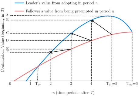
Since π(2,0)−π(0,0)> π(2,2)−π(0,2) it must be that T2L ≤ T2F. Fudenberg and Tirole (1985) shows that the value of leading in period T2L exceeds the follower’s value of adopting in period T2F so that each firm would prefer to play the role of leader. These two adoption dates (T2L, T2F) form the Reinganum (1981b) pre-commitment (i.e. Nash) equilibrium. In continuous time, the benefit from acting as leader incentivizes the follower to preempt the
leader and adopt just before T2L, thereby forcing him to take the role of follower and adopt atT2F.25 Each firm continues to preempt its competitor until it is no longer profitable, which occurs when the value of leading and following are equalized. While the logic is similar in
discrete time, the discontinuous jumps in the values of leading and following in each period
can cause the equilibrium outcome to be slightly different. Specifically, the preemption may
stop at point before the firms values are equalized, so that the leader still generates some rent
at the follower’s expense. Additionally, for certain marginal cost vectors the discontinuous
jumps in time can generate a “faulty” joint-adoption equilibrium in period T2F. We discuss these two issues in detail in Appendix B. Nevertheless, defining T2∗L as the leader’s adoption date once preemption is completed, the set of equilibria in this continuation game involve one
firm adopting in periodT2∗Land the remaining firm adopting inT2F. The equilibrium is unique up to the firm index. Figure A.5 plots the duopolists’ equilibrium j = 2 adoption dates for all potential costs entering periodT. The use of discrete time is generating the joint-adoption equilibria which would become diffusion equilibria if time periods were sufficiently short. The
overall inefficiency of the duopoly is roughly increasing inc. Three types of inefficiencies arise in the duopoly model relative to the socially optimal outcome: inefficiency created by “too
much” adoption, adoption at suboptimal dates, and setting price above marginal cost. While
j = 2 is always adopted twice in this continuation game, the additional adoption increases overall market output and decreases the market price. Ascdecreases the duopolists’ adoption dates tend to diverge from the planner’s adoption date but adoption costs are also falling.
Overall inefficiency falls because the the adoption cost for the second adopter becomes less
significant.
Equilibrium Strategies in (T,0,1,0) and (T,0,0,1)
Without loss we focus on state (T,0,1,0) and assume that firm 1 enters period T with a technological advantage. As a result, the firms’ values from acting as leader or follower in each
period are different. Slightly abusing notation, letTi2F denote firmi’s optimal period to adopt
25It is still optimal for the former leader to adopt atT
2F because it is a best-responseregardless of
j = 2, conditional on being the second firm to adopt j= 2. T12F is therefore the first period where the following inequality holds
π(2,2)−π(1,2)> C(n)−βC(n+ 1), (2.14)
and T22F is defined analogously for firm 2:
π(2,2)−π(0,2)> C(n)−βC(n+ 1). (2.15)
Comparing the LHS of these inequalities it is obvious that T22F ≤ T12F. Again, due to the use of discrete time, there exists a set of cost vectors where T22F = T12F. In these situations the equilibrium analysis is equivalent to that in state (T,0,0,0) except that firm 1’s
continuation value of leading or following is strictly greater than firm 2’s respective value due
to the technological advantage entering periodT. These differences in continuation values can generate multiple asymmetric diffusion equilibria.26
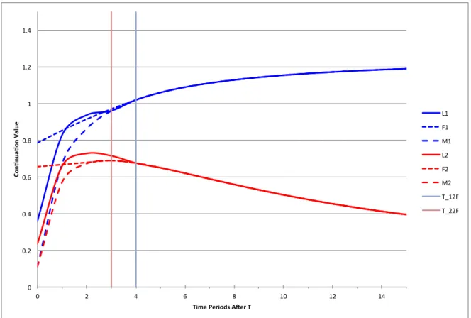
If T22F < T12F then the equilibrium strategies become slightly more complicated. To simplify the exposition we employ an example that is summarized in Table A.1 and depicted
in Figure A.6. We assume that firm 1 enters periodT with marginal costc1= 0.15 while firm 2
enters having not adoptedj= 1 (c0= 0.35). First, using (2.14) and (2.15) it is straightforward
to show that T22F =T + 3 and T12F =T + 4. Given these values I can then calculate each firm’s value (beginning in period T) under the three potential equilibria: joint adoption, firm 1 leads and firm 2 follows, and firm 2 leads and firm 1 follows. These values are summarized
in Table A.1 and are calculated such that the first adoption of j = 2 occurs in periodn and if n < Ti2F then firm i acts optimally by following in Ti2F. For instance, suppose that the first adoption of j = 2 occurs in n = 1. If both firms adopt in n= 1 then firm 1’s value is
26An example of this occurs when c
0 = 0.42 and c1 = 0.23. Here T12F = T22F = T + 3 and
T12L =T22L =T + 2. If firm 1 adopts in periodT + 2 in hopes of acting as leader, firm 2 preempts
M1 = 0.673 while firm 2’s value is M2 = 0.573. If firm 1 adopts in n= 1 and firm 2 waits to
adopt until T22F = T+ 3 then firm 1’s value is L1 = 0.829 and firm 2’s value is F2 = 0.667.
Similarly, if firm 2’s value from leading inn= 1 is L2 = 0.66 and firm 1’s value from acting as
follower isF1 = 0.853. These values are plotted for each firm in Figure A.6.
Using the logic from the previous section, it is straightforward to show that T22J < ∞ and firm 2 has a strictly dominant strategy to adopt in all periods t≥T12F, eliminating the possibility of a late joint-adoption equilibrium.27 Next, consider each periodT22F ≤t < T12F. By the definition of T12F firm 1’s value from joint adoption must be strictly less than its value from delaying adoption until T12F. Further, firm 1’s value from leading in period t is equal to the value under joint adoption because given firm 1’s decision to adopt, firm 2 has a
strictly dominant strategy to adopt as well (since t ≥T22F). As a result, the only potential equilibrium in this range involves firm 2 adopting in periodT22F and firm 1 delaying adoption until T12F. Yet, given this knowledge, firm 2 has an incentive to move its adoption time even earlier to T22L. In the example, T22L =T + 2 with an associated value of L2 = .728. Next,
we check to see if firm 1 has an incentive to preempt firm 2 in T22L−1 which is t = T + 1 in the example. If firm 1 allows firm 2 to adopt in t=T + 2 (and subsequently optimizes by adopting in T12F = T + 4) his continuation value is F1 =.914. If firm 1 preempts firm 2 in
t=T+ 1 (forcing firm 2 to optimally adopt inT22F =T+ 3) his continuation value decreases toL1 = 0.829. Thus, firm 1 has no incentive to preempt firm 2 and the unique equilibrium of
this continuation game involves firm 2 adopting j = 2 in t= T + 2 and firm 1 subsequently adopting int=T+ 4. While simulation results suggest that this type of equilibrium is unique (where firm 2 acts as the leader and firm 1 follows) ifT22F < T12F, we are struggling to prove this result in general.28
27If π(2,2)−π(1,0)<0 firm 1 prefers to delay a joint-adoption equilibrium indefinitely. However,
the fact thatt≥T12F ensures that if firm 2 adopts, firm 1’s best response is to adopt as well.
28We have attempted to prove that firm 1 has a strictly dominant strategy to choose to not adopt
in period T22L but cannot show that it is always true. We think that there are certain cost vectors
where firm 1 might be willing to preempt firm 2 but firm 2 is subsequently willing to preempt to an even earlier date. In other words, firm 2 doesn’t necessarily adopt inT22L–it might adopt at an earlier
Equilibrium Play Beginning in (0,0,0,0)
Given a marginal cost vector (c0, c1), each firm can calculate the four pertinent expected
continuation valuesEV(T,0, a, b), ∀a, b= 0,1.29 At this point it would seem logical to proceed as we did in the analysis of (T,0,0,0). However, the expected continuation values cannot be
ranked for all values of (c0, c1). As a result, differences in theEV(·)’s may have different signs,
leading to varying optimality conditions for the adoption ofj= 1. Ultimately we will need to consider several different cases which are explained in detail below.
First consider the situation where one firm has adopted j = 1 and the competing firm is deciding whether or not to adopt. In period t, the follower’s Bellman equation is
V(t, t,0,1) = max at∈{0,1} π(a
t,1)−1[
at6=at−1]C(t)+β[ρEV(T,0, at,1)+(1−ρ)EV(t+1, t+1, at,1)].
Again, the follower is faced with a simple optimal stopping problem due to the strictly
decreas-ing and strictly convex nature of C(t). So, applying the same logic used to derive (2.7) and (2.10), the follower waits to adoptj = 1 until the first periodt where the following inequality holds:
π(1,1)−π(0,1) +βρ[EV(T,0,1,1)−EV(T,0,0,1)]
| {z }
x
> C(t)−β(1−ρ)C(t+ 1). (2.16)
In the efficient and monopoly cases we proved that the difference in continuation values (term
“x” above) was positive. Or stated differently, the continuation value was increasing in the
planner’s/monopolist’s technology. However, in a duopoly market this is not always the case.30
shown to be true for 0.5> c0> c1), we cannot show that this outweighs the higher cost of adopting at
an earlier date.
29While all uncertainty is technically resolved at the beginning of periodT, there is still the potential
issue of multiple equilibria. Thus, EV(T,0, a, b) is the average continuation value for a firm entering periodT with technology “a” (and competitor’s technology “b”) across all equilibrium outcomes. Any marginal cost vector generates a maximum of two pure strategy equilibria in the continuation game beginning inT. If multiple equilibria exist they are generated by each firm wanting to act as leader in periodT2F−1 in states (T,0,0,0) and T22F −1 in state (T,0,1,0).
30Setting β= 0.9 andC(t) = 1/(1 +t) we found that 84 of the 1176 marginal cost vectors analyzed
IfEV(T,0,1,1)−EV(T,0,0,1)<0, the follower’s optimal adoption date forj = 1 is pushed far into the future and if the difference is significant, so that the entire LHS of (2.16) is
negative, the follower will find it optimal to never adopt j = 1. Further, while we showed in the analysis of the continuation game beginning in (T,0,0,0) it must be that T2F ≤ T2J, that isn’t necessarily true for j = 1. Defining T1J as the optimal date for the two firms to jointly adoptj= 1, it is straightforward to show thatT1J is the firsttsatisfying the following condition:
π(1,1)−π(0,0) +βρ[EV(T,0,1,1)−EV(T,0,0,0)]> C(t)−β(1−p)C(t+ 1). (2.17)
Whileπ(0,0)> π(0,1), it may be thatEV(T,0,0,1)> EV(T,0,0,0) so that the LHS of (2.17) is greater than the LHS of (2.16) and T1J ≤ T1F. While this is a departure from Fudenberg and Tirole (1985) who explicitly show that T1J ≥T1F using a quasiconcavity argument, it is still straightforward to characterize the firms’ equilibrium strategies in this case. IfT1J =T1F then both firms have a strictly dominant strategy to adoptj= 1 in all periodst≥T1J =T1F. From that point backwards-induction can be used to solve for the firms’ equilibrium strategies
in all t < T1J using logic similar to that employed in (T,0,0,0) continuation game. Next, consider T1J < T1F. InT1F the firms again have a strictly dominant strategy to adopt j= 1 in all potential states. In all periodsT1J ≤t < T1F a joint adoption equilibrium will occur in state (t, t,0,0) but the follower will delay adoption untilT1F if the leader has already adopted. However, state (T1J, T1J,0,0) will never be reached in equilibrium if there exists a period t < T1J where the value of leading exceeds the value of joint adoption at T1J. If this date (T1L) exists then a diffusion equilibrium will ensue where the leader’s actual date of adoption
may occur before T1L due to the preemption incentive. However, the inability to rank the EV(·)’s prevents us proving the existence of T1Lin general.
The real difficulties for this analysis arise when T1F,T1J, or both values equal∞ (i.e. the LHS of (2.16), (2.17), or both are negative). In what follows we describe the algorithm used
(1−ρ) the firms believe that they will transition to state (T, T, aTi−1, aT−−i1), which we have not solved for at that point in the backwards-induction process (because working backwards
from the end of the game to T this state does not exist). To calculate EV(T, T, aTi−1, aT−−i1) we need to determine the hypothetical date when all firms have a strictly-dominant strategy
to adopt j = 1.31 The fact that this hypothetical date is potentially infinite (if at least one
firm has a strictly) is what generates the following cases:
Case 1: Both T1F and T1J are finite
• Determine which date is greater and start the backwards induction from that point
• In all potential states entering that date each firm has a strictly dominant strategy to
adoptj= 1 (by the definition of T1F and T1J)
• Using stationarity it is straightforward to solve for each firm’s value in this hypothetical
last period:
EV(¯t,¯t, a¯ti−1, a−t¯−i1) =π(1,1)−1h
a¯t i6=a
¯
t−1
i
iC(n)+
β
ρEV(T,0,1,1) + (1−ρ)π(1,1) +βρEV(T,0,1,1) 1−β(1−ρ)
,
where ¯t=max{T1F, T1J}
Case 2: T1F is finite but T1J is infinite
• The analysis here is similar to that used for the continuation game beginning in state
(T,0,0,0). From the previous analysis we know that there can be no joint adoption
equilibrium afterT1F when time is discrete.
• If one firm has adoptedj = 1 at an earlier date then we know the remaining firm responds optimally by adopting inT1F and the values are the same as in Case 1
31For instance, suppose that T = 10 butT
1F = 14. Conditional on being preempted at some date
• If both firms enter T1F having not adopted j = 1 then it must be that either both or neither of the firms want to adopt j = 1 (because if only one firm adopts j = 1, by the definition of T1F the non-adopter would want to adopt as well). If joint-adoption is optimal, values are calculated as in Case 1. If not, each firm’s value is:
EV(T1F, T1F,0,0) =π(0,0) +β
ρEV(T,0,0,0) + (1−ρ)π(0,0) +βρEV(T,0,0,0) 1−β(1−ρ)
Case 3: T1J is finite but T1F is infinite
• If both firms enter periodT1J with j = 0 then a joint-adoption equilibrium ensues and each firm earns the value in Case 1
• If one of the two firms has adopted then the remaining firm finds it optimal to never
adoptj= 1. The continuation value for the adopting firm is:
EV(T1J, T1J,1,0) =π(1,0) +β
ρEV(T,0,1,0) + (1−ρ)π(1,0) +βρEV(T,0,1,0) 1−β(1−ρ)
and the continuation value for the non-adopting firm is:
EV(T1J, T1J,0,1) =π(0,1) +β
ρEV(T,0,0,1) + (1−ρ)π(0,1) +βρEV(T,0,0,1) 1−β(1−ρ)
.
Case 4: Both T1F and T1J are infinite
• In this situation states (t, t,1,0), (t, t,0,1), and (t, t,1,1) are all temporarily stationary
until j= 2 is released. The values in these states are calculated using the correct forms from Cases 1-3.
• While joint-adoption is not optimal, it may be true that a single firm would find it
optimal to adopt in state (t, t,0,0). So, we solve for the earliesttsuch that a single firm would find it optimal to adopt. This occurs in the smallest t such that the following inequality holds:
If this condition is not satisfied for a very large value of t32 then we assume that neither firm will adopt j = 1. If the condition is satisfied then there are two equilibria in state (TL, TL,0,0): one in which firm 1 adopts and firm 2 does not adopt and another where the indices are reversed. In this case we simply pick one of the two equilibria and begin
working backwards fromT1L.
For each case we now have a way of “closing” the j = 1 and can work backwards to calcu-late the value of V(T, T, aTi−1, aT−−i1) for every combination of actions. With this value the backwards-induction process can be continued until we reach t = 0. The presence of these different cases makes it very cumbersome to discuss the equilibrium adoption dates forj= 1. Without imposing additional assumptions on C(n) and the ranking of both the EV(·)’s and the differences in EV(·)’s we cannot make any general comment on the equilibrium adoption dates. However, we run a variety of simulations to illustrate the dynamics of the technology
adoption game. There are at most four pure strategy Markov perfect equilibria in the dynamic
game. Since firms are ex ante identical all of the equilibrium adoption dates of j= 1 are nec-essarily isomorphic in the sense that if in one equilibrium firm 1 adoptsj= 1 in periodx and firm 2 adopts in period y then the other equilibrium involves firm 1 adopting in y and firm 2 adopting in x. If both firms enter period T with the same technology then the equilibrium adoption dates in that subgame are also necessarily symmetric. However, as previously
dis-cussed in section 2.2.3, if one firm enters periodT with a technological advantage then multiple equilibria need not be symmetric.
2.3 Simulations
In this section we examine the equilibrium properties of the model for a variety of
parameter-izations. Before discussing all of the simulations in detail it is helpful to highlight some of the
main results which are bulleted below:
• Leap-frogging behavior is most likely when the adoption cost function is relatively flat
and the first advancement is relatively large. In this situation there is a large preemption
incentive for the first technology but once preempted the remaining firm has little
incen-tive to adopt. However, the preempted firm (if it does not adopt the first technology)
has a much higher marginal benefit from adopting the second technology. If the adoption
cost function declines faster there is a greater chance that both firms will find it optimal
to adopt the first technology.
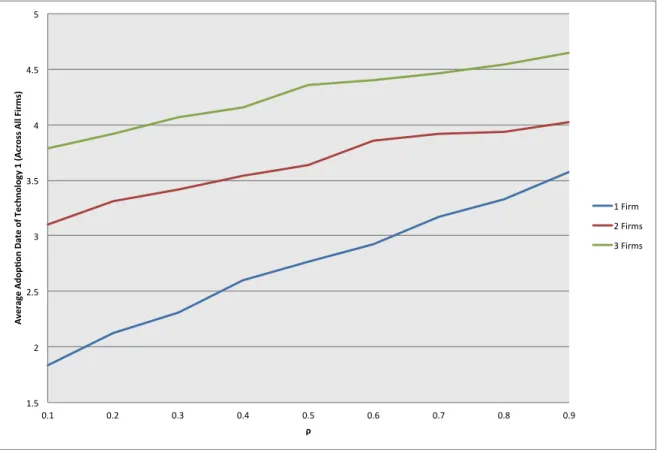
• Asρ increases both firms tend to delay the adoption of the first technology. The effect is most evident when the first advancement is relatively small (i.e. high values ofc0−c1)
and the adopt cost function is relatively flat. However, when the adoption cost function
is significantly convex and the first advancement is large, changes inρmay have no effect on the equilibrium adoption dates of the first technology.
• Inefficiency in the model is caused by suboptimal adoption dates, too much adoption,
and setting price above marginal cost. Only rarely does the preemption incentive drive
a duopolist to adopt before the planner’s adoption date. Total inefficiency is largest
for high values of (c0−c1) where both duopolists adopt the first technology relatively
early. Further, when (c0−c1) is high and adoption costs are relatively flat, a monopoly
market is more efficient than a duopoly market. However, the relationship between total
inefficiency and (c0−c1) is not monotonic.
• For most marginal cost vectors a steeper adoption cost function will result in lower total
inefficiency. While the adoption average adoption date of the first technology decreases,
adoption costs decrease at a faster rate.
• Ceteris paribus, as ρ increases (i.e. the firms believe that the second advancement is more imminent) the duopoly inefficiency tends to decrease as firms delay the adoption
of the first technology.
• Comparing a one-technology model with a two technology model, there is no systematic
relationship between firms’ adoption dates of j = 1. However, as c0 −c1 increases,
the leader and follower’s adoption dates in the two-technology model (very roughly)