Ou_unc_0153D_15576.pdf

(1)

QUANTILE REGRESSION MODELS FOR INTERVAL-CENSORED FAILURE TIME DATA

Fang-Shu Ou

A dissertation submitted to the faculty at the University of North Carolina at Chapel Hill in partial fulfillment of the requirements for the degree of Doctor of Philosophy in the

Department of Biostatistics in the Gillings School of Global Public Health.

Chapel Hill 2015

(2)

c ○ 2015 Fang-Shu Ou

(3)

ABSTRACT

Fang-Shu Ou: Quantile Regression Models for Interval-censored Failure Time Data (Under the direction of Jianwen Cai and Donglin Zeng)

Quantile regression models the conditional quantile as a function of independent vari-ables providing a complete association between the response and predictors. Quantile regression can describe the association at different quantiles yielding more information than the least squares method which only detects associations with the conditional mean. Quantile regression models have gained popularity in many disciplines including medicine, finance, economics, and ecology as they can accommodate heteroscedasticity.

A specific type of failure time data is called interval-censored where the failure time is only known to have occurred between certain observation times. Such data appears com-monly in medical or longitudinal studies because disease onset is known to have occurred between scheduled visits but the exact time is unknown. Quantile regression has been ex-tended to survival analysis with random censoring time. Most methods focus on survival analysis with right-censored data while a few were developed for data with other censoring mechanisms. Despite the fact that the development for censored quantile regression flour-ishes, limited work has been done to handle interval-censored failure time data under the quantile regression framework.

(4)

(5)

To Nyan-Mei Wang, my mother and the source of unconditional love and support. To Martin Andrew Heller, my husband and my best friend.

(6)

ACKNOWLEDGMENTS

I would like to express my sincere gratitude to my advisers Dr. Jianwen Cai and Dr. Donglin Zeng, for their guidance and support throughout my graduate studies. They gave me the freedom to explore different possibilities, learn from my own mistakes, and pointed me in the right direction when I have gone astray. I cannot ask for better advisers than them. Additionally, I would like to thanks my committee members, Dr. David Couper, Gerardo Heiss, and Haibo Zhou, for their time and insightful comments.

I would like to offer thanks to my supervisors Drs. Daniela Sotres-Alvarez and Diane Catellier while working at the Collaborative Studies Coordinating Center and Dr. June Stevens in the Nutrition Department. They provided not only the financial support for my study but also the opportunity to work on interesting research projects.

(7)

TABLE OF CONTENTS

LIST OF TABLES ... x

LIST OF FIGURES ... xii

CHAPTER 1: INTRODUCTION ... 1

CHAPTER 2: LITERATURE REVIEW ... 4

2.1 Quantile Regression... 4

2.1.1 Estimation ... 9

2.1.2 Inference... 14

2.2 Censored Quantile Regression ... 18

2.3 Accelerated Failure Time Models for Interval-Censored Failure Time Data ... 26

CHAPTER 3: QUANTILE REGRESSION MODELS FOR CURRENT STATUS DATA ... 32

3.1 Introduction ... 32

3.2 The Method ... 34

3.2.1 Model and Data ... 34

3.2.2 Parameter Estimation and Algorithm... 36

3.3 Asymptotic Properties... 41

3.3.1 Identifiability... 41

3.3.2 Consistency ... 42

(8)

3.4 Numerical Studies ... 44

3.4.1 Simulation... 44

3.4.2 Application... 51

3.5 Discussion ... 55

3.6 Proof of lemma and theorems... 57

CHAPTER 4: QUANTILE REGRESSION MODELS FOR CASE II INTERVAL-CENSORED FAILURE TIME DATA ... 66

4.2 Model and Inference Procedure ... 68

4.2.1 Models and Data ... 68

4.2.2 Parameter Estimation and Algorithm... 69

4.3.1 Identifiability... 75

4.3.3 Asymptotic Distribution ... 77

4.4 Simulation Studies ... 78

4.5 Application ... 79

4.7 Proofs of Lemma and Theorems ... 88

CHAPTER 5: SEMIPARAMETRIC METHODS FOR AC-CELERATED FAILURE TIME MODELS FOR INTERVAL-CENSORED DATA... 98

5.2 Model and Inference Procedure ... 100

5.2.1 Models and Data ... 100

(9)

5.3.2 Asymptotic Distribution ... 105

5.4 Simulation Studies ... 106

5.5 Application ... 109

CHAPTER 6: SUMMARY AND FUTURE RESEARCH... 126

(10)

LIST OF TABLES

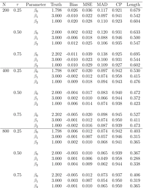
3.1 Simulation results for Simulation 1, based on 1000

simulation replicates. ... 48

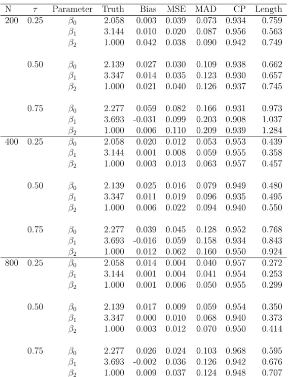
3.2 Simulation results for Simulation 2, based on 1000 simulation replicates. ... 49

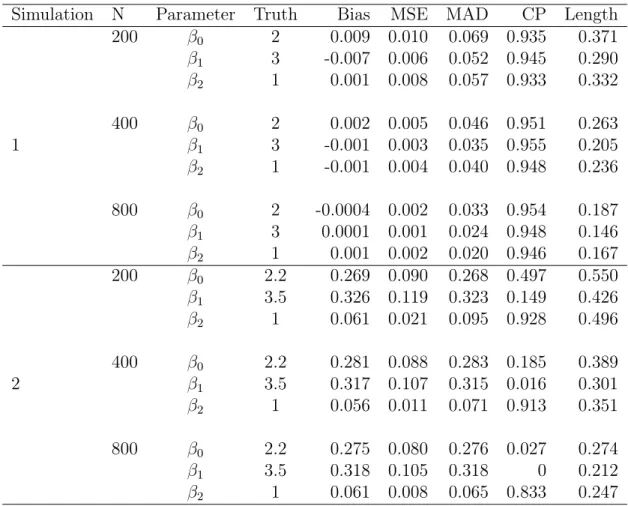
3.3 Results from accelerated failure time models with nor-mal error, based on 1000 simulation replicates... 50

3.4 Results of analyzing “The Voluntary HIV-1 Counsel-ing and TestCounsel-ing Efficacy Study Group” data, effect on delaying STD contraction in months. ... 54

4.7 Results of analyzing “Atherosclerosis Risk in Commu-nities (ARIC) study” data, effect on time to hyperten-sion onset in years ... 84

5.8 Normal distribution, N=200 ... 114

5.11 Logistic distribution, N=200 ... 117

5.14 Extreme-value distribution, N=200 ... 120

5.17 Relative efficiency... 123

(11)

(12)

LIST OF FIGURES

2.1 A scatterplot of 71 observations of stream width to depth ratio and trout densities with 0.95, 0.75, 0.50, and 0.25 quantiles (dash line) and least squares

re-gression (solid line) estimates for the modellog(trout densit) =

β0+β1width:depth+ε. ... 6

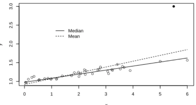
2.2 A toy example. A scatterplot of 38 observations and median (solid line) and least squares (dash line) esti-mates. The solid dot is served as an outlier... 6

2.3 Quantile regression for birth. ... 8

2.4 Quantile regression for birth (continued). ... 8

2.5 Effect of mother’s weight gain... 9

2.6 Quantile regression loss function... 10

2.7 Huber function approximation of a quantile regres-sion loss function. Dashed line is the Huber function approximation and the solid line is the quantile loss function. ... 15

3.8 An illustration of using the difference between two hinge loss functions to approximate a 0/1 loss. A smaller provides a closer approximation. ... 37

3.9 Days between baseline visit and first follow-up for 903 females in voluntary counseling and testing (VCT) and basic health information (BHI). ... 52

3.10 Nonparametric maximum likelihood estimator (NPMLE) of the (unobserved) failure time distribution function stratified by voluntary counseling and testing (VCT) vs. basic health information (BHI) and age (below or above median age). ... 52

(13)

4.12 An illustration of using the difference between two

hinge loss functions to approximate a 0/1 loss... 71 4.13 Nonparametric maximum likelihood estimator (NPMLE)

of the (unobserved) failure time distribution function

stratified by covariates. ... 83 4.14 ARIC data: effect on time to hypertension onset. The

vertical bars are symmetric confidence interval

con-structed using a subsampling method. ... 85 5.15 Nonparametric maximum likelihood estimator (NPMLE)

of the (unobserved) logarithm of time to calcification

distribution function stratified by covariates. ... 110 5.16 Nonparametric maximum likelihood estimator (NPMLE)

of the (unobserved) logarithm of failure time distribu-tion funcdistribu-tion for patients received radiadistribu-tion therapy alone (RT) and patients received radiation therapy

(14)

CHAPTER 1: INTRODUCTION

Regression analysis has typically been performed using the least squares method since the time of Gauss. The least squares method summarizes the relationship between the de-pendent variable and indede-pendent variables by a conditional mean function. When the homoscedasticity assumption fails; however, the least squares method cannot provide a complete picture of the relationship between the response and predictors.

Quantile regression, on the other hand, models the conditional quantile as a function of independent variables providing a solution when heteroscedasticity is present and offers a more detailed perspective regarding associations. The conditional median is less sensitive to skewness than the conditional mean making it a more reliable measure of the central tendency. When there is heteroscedasticity, quantile regression can describe the association at different quantiles yielding more information than the least squares method which only detects associations with the conditional mean. Quantile regression models have gained popularity in many disciplines including medicine, finance, economics, and ecology as they can accommodate heteroscedasticity. In survival analysis, ease of interpretation is partic-ularly appealing since the estimates can be directly interpreted as the effect on survival time.

(15)

A specific type of failure time data is called interval-censored where the failure time is only known to have occurred between observation times. Such data appears commonly in medical or longitudinal studies because subjects schedule follow-ups where disease status is determined. The disease then is known to have manifested between scheduled visits but the exact time is unknown. There are two subtypes of interval-censored data, Case I and Case II. Case I interval-censored data refers to interval-censored failure time data where all observed intervals had either zero or infinity as one of the end points, i.e. all observa-tions are either right- or left-censored. Case II interval-censored data is interval-censored failure time data where we know the event occurred either prior to the first observation time, between observation times, or after the final observation time. Despite the fact that the development for censored quantile regression flourishes, only one published manuscript discussed the method developed to handle interval-censored failure time data under the quantile regression framework. This existing publication did not provide any theoretical justification regarding the method proposed and can only handle categorical covariates in the model.

(16)

follow-up; therefore, it is a typical Case I interval censored failure time data.

The Atherosclerosis Risk in Communities Study is a prospective epidemiologic study with five follow-up visits. During each visit, the disease status, such as diabetes, hyper-glycemia, and hypercholesterolemia, was determined using biomarkers. If a biomarker value exceed a certain threshold then the participant was diagnosed as having the disease. Accordingly, we only know the disease occurred between the last and the current follow-up but the exact onset time is unknown; thus, it is Case II interval-censored data. We ex-tended our method developed for Case I interval-censored data to Case II data and applied it on the data from Atherosclerosis Risk in Communities Study.

(17)

CHAPTER 2: LITERATURE REVIEW

2.1 Quantile Regression

The first attempt of regression analysis using least absolute deviations may be dated back to 1760 by the Croatian Jesuit Roger Boscovich who was interested in a problem con-cerning ellipticity of the earth and a geometric algorithm was proposed as the solution. Boscovich’s proposed method is a peculiar hybrid of mean and median ideas, i.e. the inter-cept is estimated as a mean and the slope is estimated as a median. With the development of the least squares at the end of the 18th century, Boscovich’s estimator faded into his-tory. Until a century later, Francis Ysidro Edgeworth modified Boscovich’s conditions and proposed to minimize the sum of absolute residuals. A geometric algorithm was developed for the bivariate case but the approach was rather awkward. The least absolute deviation method did not become practical on a large scale until the simplex algorithm for linear programming was developed in the late 1940s. Koenker (2005) and Portnoy et al. (1997) provide interesting historical introductions to least absolute deviations.

The τth quantile of a random variable, Y, is defined as

Qτ(Y) = inf{y :FY(y)≥τ},

(18)

allowing an intercept in the model, the τth conditional quantile is defined as

Qτ(Y|X =x) = inf{y :FY(y|x)≥τ},

where FY(y|x) denotes the conditional cumulative distribution function of Y givenX =

x. Similarly to the least squares method which fits the conditional means as a function of

covariates, the linear quantile regression model fits the conditional quantile as a function of covariate, i.e.

Qτ(Y|X) = X0β(τ),

where β(τ)is the quantile coefficient that may depend on τ. β(τ) can be interpreted as the marginal change in the τth _{quantile caused by an increase in covariate values.}

Several advantages of quantile regression are worth mentioning. Quantile regression provides a complete picture of the relationship between response variable and covariates; therefore, it can detect relationships which may be overlooked by the least squares method. It is robust to outliers in response variable and the estimation and inference are distribution-free. For example, Dunham et al. (2002) analyzed the relationship between the abundance of Lahontan cutthroat trout and the ratio of stream width to depth. While a least squares regression estimated no linear change in mean density across ratio, the quantile regression estimates shows a nonlinear, negative relationship of cutthroat trout densities across 13 streams and over 7 years in the upper quantiles (Figure 2.1).

Figure 2.2 shows a toy example to demonstrate the robustness of quantile regression when outliers are present. The data was generated from a linear regression model with iid normal error with one additional data point (solid dot) added as an outlier. The 0.5 quantile (median) estimate is denoted by the solid line and the least square estimate is denoted by the dash line. It is clear that the median fit was not influenced by the outlier.

(19)

● ● ● ● ● ● ● ●● ● ● ● ● ●_● ● ●● ● ● ● ● ● ● ●●● ● ● ● ● ● ● ● ● ● ● ● ● ● ● ● ● ● ● ● ● ● ● ● ● ● ● ● ● ● ● ●● ● ● ● ● ● ● ● ● ● ● ● ●

10 20 30 40 50

0.0 0.5 1.0 1.5 Stream width:depth T

rout per m of stream

Least Squares tau=0.25 tau=0.50 tau=0.75 tau=0.95

Figure 2.1: A scatterplot of 71 observations of stream width to depth ratio and trout densities with 0.95, 0.75, 0.50, and 0.25 quantiles (dash line) and least squares regression (solid line) estimates for the model log(trout densit) = β0 +β1width:depth+ε.

● ● ● ● ● ● ● ● ● ● ● ● ● ● ● ● ● ● ● ● ● ● ● ● ● ● ● ● ● ● ● ● ● ● ● ● ● ●

0 1 2 3 4 5 6

1.0 1.5 2.0 2.5 3.0 x y ● Median Mean

(20)

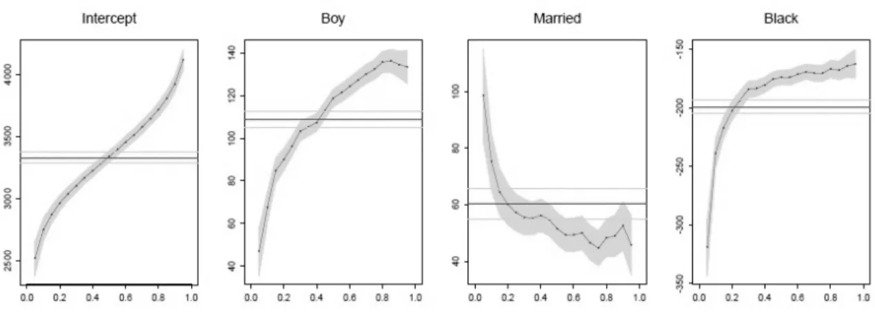
investigation carried out by Abrevaya (2002). The outcome of interest was infant birth weight and the covariates included were various demographic characteristics and maternal behavior. Please see Koenker (2005) for a detailed description of the data source, covari-ates used, and quantiles estimated. The data has been centered to yield a reference group, a girl born to an unmarried, white mother with less than a high school education, who is 27 years old and had a weight gain of 30 pounds, did not smoke, and had her first prena-tal visit in the first trimester of pregnancy. Since the data has been centered, the inter-cept of the model (far left panel of Figure 2.3) can be interpreted as the estimated condi-tional quantile function of the birth-weight distribution of the reference group. The me-dian birth-weight of the reference group is about 3300 grams and the 5th percentile of the birth-weight is about 2500 grams which is the conventional definition of a low-birth-weight baby.

The far right panel of Figure 2.3 shows the difference in birth-weight of infants born to black versus white mothers. The birth-weight of infants born to black mothers is signifi-cantly less than those born to white mothers, especially in the lower tail of the distribu-tion. At the 5th percentile of the conditional distribution, infants born to black mother are more than 300 grams lighter than infants born to white mother. The horizontal line indi-cates the results from ordinary least-squares which would conclude that the birth-weight of infants born to black mothers are about 200 grams less on average than those born to white mothers.

(21)

Figure 2.3: Quantile regression for birth.

more complete picture of the relationship between a mother’s weight gain and infant birth-weight. Figure 2.5 shows the marginal effect of mother’s weight gain for all quantiles eval-uated at four specific levels of mother’s weight gain. These 4 levels are roughly the 10th, 25th, 75th, and 90th percentile of mother’s weight gain.

Figure 2.4: Quantile regression for birth (continued).

(22)

of Figure 2.5). For mothers who already gained about 40 pounds, each additional 1 pound of weight gain would only increase infant weight by about 5 to 10 grams. The ability to draw conclusions at a specific quantile of interest is the advantage of using quantile regres-sion.

0.2 0.4 0.6 0.8

5 10 20 30 Quantile gr ams ● ● ● ● ● ● ● ● ● ● ● ● ● ● ● ● ● ● ● Mother's Weight Gain 15 Lbs

0.2 0.4 0.6 0.8

Figure 2.5: Effect of mother’s weight gain.

Unlike the least squares method, quantile regression models are invariant to monotone transformations (Koenker 2005). Specifically, let h(·)be a monotone nondecreasing func-tion on<, then for any random variable Y, Qh(Y)(τ) = h(QY(τ));that is, the quantiles of the transformed random variable h(Y)are simply the transformed quantiles of the original

Y. This property is immediate from the elementary fact that, for any strictly monotone h, P(Y ≤y) =P(h(Y)≤h(y)).

2.1.1 Estimation

(23)

the following function,

min β∈Rp

n

X

i=1

|yi−x0iβ|, (2.1)

where {y1,· · · , yn} is the random sample and xi is the covariates associate with random sample yi where the first component of xi is a constant one. Koenker and Bassett (1978) generalized the median regression to the τth quantile (₀ _{< τ <} ₁) by simply replacing the absolute value in Equation (2.1) with the loss function, ρτ(·), i.e.

min β∈Rp

n

X

i=1

ρτ(yi−x0iβ), (2.2)

where the quantile loss function is defined as

ρτ(u) = u(τ−I(u <0)) (2.3)

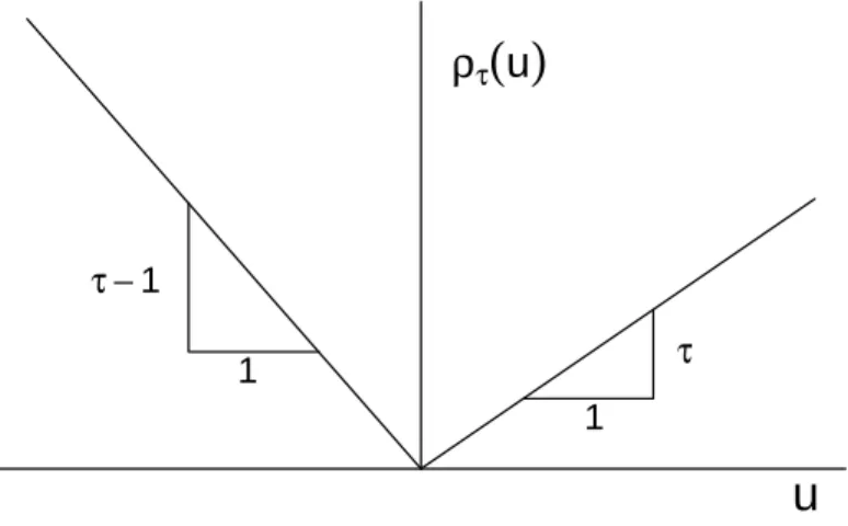
The piecewise linear loss function, ρτ(·)is illustrated in Figure 2.6.

ρ

τ(

u

)

τ −1

1 τ

1

u

Figure 2.6: Quantile regression loss function

(24)

Simplex Algorithm Equation (2.2) is equivalent to

min

β∈Rp





X

i∈{i:yi≥xiβ}

τ|yi−x0iβ|+

X

i∈{i:yi<x0_iβ}

(1−τ)|yi−x0iβ| 



= min

β,u,vτ1

0

nu+ (1−τ)1

0

nv (2.4)

such that y−x0β =u−v,β ∈Rp, and u≥0,v ≥0,

where y = (y1,· · · , yn)0,x = (x1,· · ·, xn)0,1n is a (n × 1)vector of the value 1, and

(·)+ denotes the positive part. Taking this one step further, let φ = (β)+, ψ = (−β)+,

B = [x −x I −I], θ = (φ0, ψ0, u0, v0)0, and d = (00,00, τ1_n0 ,(1− τ)10_n)0 where 00 = (0,0,· · · ,0)p). We may reformulate the problem as a standard linear programming minimization problem with primal form:

min

θ d

0_θ _{such that} _Bθ ₌_y, _θ_≥₀_.

Thus, the Equation (2.2) may be solved using the simplex method. The simplex method starts at a feasible vertex and travels from vertex to vertex along the edge of the polyhe-dral constraint set. The path is chosen by the steepest descent and the algorithm contin-ues until arriving at the optimum.

In the special case when τ = 0.5, i.e. median regression, the simplex method algo-rithm developed by Barrodale and Roberts (1973) is often used for solving the optimiza-tion problem since it appears to be superior computaoptimiza-tionally to other algorithms. The Barrodale and Roberts algorithm is implemented in two stages. Stage 1 only chooses the columns in x or−x as pivotal column during the firstp iterations. Stage 2 interchanges

nonbasic columns with basic columns in I or −I. The basic columns in x and −xare

forced to remain in the basis during Stage 2. Stage 1 will be executed p times and Stage

(25)

Roberts algorithm can be extended for any given quantile as described by Koenker and d’Orey (1987). The simplex method provides an extremely efficient solution to quantile re-gression when the dataset size is moderate, for example, less than 5000 observations and 50 covariates. However, the computational speed became unsatisfactory for large datasets.

Interior Point Algorithm To overcome the computational difficulty of the simplex method when the dataset is large, interior point algorithms for linear programming were applied to quantile regression. Instead of traveling along the exterior of the constraint set, Newton steps were taken within the interior of a deformed constraint set toward the boundary. Consider the canonical linear program

min{c0x |Ax=b, x ≥0} (2.5)

and assume that there is a strictly feasible solution in the interior of the constraint set. One way to find the solution is to decrease c0x while ensuring the boundary of the feasible

set is not crossed. We can achieve this by augmenting the objective function by a logarith-mic barrier term. Let

B(x, µ) =c0x−µXlog(x),

and we would minimize B(x, µ|Ax = b) while reducing µto zero. The inequality

con-straints in Equation (2.5) is replaced by the penalized log barrier, thus minimizing

B(x, µ|Ax =b)by taking the Newton steps

min q

c0q−µ q0X−11n+ 1 2µ q

0

X−2q|A q = 0

(26)

where X =diag(x) =         

x1 0 · · · 0 0 x2 · · · 0 ... ... ... ... 0 0 · · · xp

         .

To use the logarithm barrier for quantile regression, we first rewrite the linear program-ming problem (Equation (2.4)) in its dual representation,

max λ {y

0

λ|X0λ= 0, λ∈[τ −1, τ]n},

or, by setting a =λ+ 1−τ,

max a {y

0

a|X0a = (1−τ)X01n, a∈[0,1]n}. (2.6)

Adding slack variables, s, such thata+s= 1n, we have the barrier function

B(a, s, µ) =y0a+µX

i

(logai+logsi),

and the Newton steps

max δa

{y0δa+µδa0(A

−1₋_S−1₎₁ n−

1 2µδ

0

a(A

−2 ₊_S−2₎_δ a}

such that X0δa= 0 where A=diag(a) and S =diag(s).

(27)

Smoothing Algorithm When a dataset is large, another suitable estimation method is found through smoothing. The original non-differentiable objective function in Equation (2.2) can be approximated by a smooth Huber function (Huber 1973) to create the objec-tive function,

min β∈Rp

n

X

i=1

Hγ,τ(yi−x0iβ), (2.7) where

Hγ,τ(t) =



      

      

t(τ −1)− 1

2(τ −1)

2_γ if _t_≤₍_τ ₋₁₎_γ

t2_/₍₂_γ₎ if ₍_τ₋₁₎_γ _≤_t_≤_{τ γ}

tτ − 1 2τ

2_γ if _t_≥_{τ γ}

and theγ is a positive real number referred to as the “threshold”. Hγ,τ(·) is a continuous differentiable function, as illustrated in Figure 2.7. The minimizer of Equation (2.7) is close to the minimizer of Equation (2.2) when γ is small and will produce the proper

es-timator before γ converge to zero. The smooth approximation method was originally

de-veloped by Madsen and Nielsen (1993) to solve linear L1 estimation problems and was fur-ther extended by Chen (2007) to general quantile regression. The computational speed of the smoothed function is comparable to interior point method and is superior for a “fat” dataset, i.e. when the ratio of covariates to observations is greater than 0.05 and whenxx0

is a non-sparse matrix (Chen 2007).

2.1.2 Inference

Methods to perform inference of quantile estimators can be separated into three types, namely direct estimation, inversion of a rank test, and resampling based methods. We will review the basic idea behind each method and compare their strengths and weaknesses.

Direct Estimation Consider the simplest case of

(28)

ρ

τ

H

_{γ, τ}

(τ −1)γ τγ

Figure 2.7: Huber function approximation of a quantile regression loss function. Dashed line is the Huber function approximation and the solid line is the quantile loss function.

where i indexes subject, yi is the response, xi is the covariate, and {ui}are iid F with den-sity f and the density in a neighborhood of τ is greater than 0 (i.e. f(F−1₍_τ₎₎ _> ₀). Un-der mild conditions, Koenker and Bassett (1978) showed

√

n( ˆβ(τ)−β(τ))→ Nd (0, w2(τ, F)D−1),

where β(τ) = β +F−1₍_τ₎_e

1, e1 = (1,0,· · · ,0)0, w2(τ, F) = τ(1− τ)/f2(F−1(τ)), and

D= limn→∞n−1P_ixix0i.

When the error terms are non-iid; however, the asymptotic behavior of _βˆ₍_τ₎ _{is more} complicated and it takes on the sandwich form (Koenker and Machado 1999)

√

n( ˆβ(τ)−β(τ))→ Nd (0, τ(1−τ)H−1J H−1),

where J(τ) = limn→∞n−1P_ixix0i and H(τ) = limn→∞n−1P_ixix0ifi(Fi−1(τ)).

(29)

depend on how dense the observations are near the quantile of interest. In the iid case, the estimation of the sparsity function is well developed (Siddiqui 1960, Bofingeb 1975, Sheather and Maritz 1983, Welsh 1988, Hall and Sheather 1988). For the non-iid case, the estimation of Hn may be performed either using an extension of the methods used for the iid case (Hendricks and Koenker 1992) or by a method based on kernel density estimation (Powell 1991).

Inversion of a Rank Test Since direct estimation requires estimation of nuisance parameters (i.e. H), a method which provides a valid test without estimating H could

be beneficial. The inversion of a rank test developed by Gutenbrunner et al. (1993) does avoid estimation of Hn.

Gutenbrunner and Jurecková (1992) observed that H´ajek-Sidˇ ´ak rankscores (Hájek et al. 1967) may be viewed as a special case of a more general form for linear model. By invert-ing the test, confidence intervals can be efficiently computed for quantile estimators.

Consider the model Qτ(Y|X1, X2) =X1β1+X2β2 and a test for the null hypothesis

H0 :β2 =ξ vs. H1 :β2 6=ξ where ξ is q-dimensional and τ is fixed. Under the null hypoth-esis and using the dual representation of Equation 2.6, the linear programming problem can be solved using

ˆ

a(ξ) = max

a {(Y −X2ξ)

0

a|X₁0a= (1−τ)X₁01n, a∈[0,1]n}.

The rank test statistic is defined as

Tn=Sn(ξ)0(τ(1−τ)q2n)

−1_S

n(ξ)→d χ2q,

where q2

n=n−1X20(I−X1(X10X1)−1X10)X2,

Sn =n−1/2X20ˆbn(ξ) d

(30)

under the null withˆ_b

n(ξ) = ˆa(ξ)−(1−τ). We can rejectH0 if Tn(ξ)> χ2(q,1−α).

Confidence intervals for β2 may be constructed by inverting the rank test. Different values of ξ can be tested and the collection of allξ for which the null hypothesis is not

rejected forms an approximate (1−α)-th confidence interval for β2. A more detailed

devel-opment of this test can be found in Gutenbrunner et al. (1993).

The most important feature of this approach is that it is scale invariant and; therefore, avoids estimation of the sparsity function. The test can be carried out in conjunction with the simplex method (Koenker and d’Orey 1994).

Resampling Based Methods There are quite a few implementations of resampling methods for quantile regression inference. There are four basic types, namely, the x-y pair

bootstrap, residual bootstrap, Markov chain marginal bootstrap (MCMB), and distinct resampling method devised by Parzen et al. (1994).

The x-y pair bootstrap resamples x-y pairs from the original dataset with replacement.

The sampled data uses the original design points; therefore, it is able to accommodate some heteroscedasticity. A slight variation of the x-y pair bootstrap was introduced by

Rao and Zhao (1992) and Chatterjee et al. (2005). Their methods also resample x-y pairs

with replacement but then each of the bootstrapped observations is weighted by a ran-domly generated weight for estimation. Commonly used random variables for generating random weights are the exponential distribution with rate parameter equal to one and Poisson(1) since their mean and variance are both one.

(31)

The Markov chain marginal bootstrap (MCMB) was developed by He and Hu (2002) and it reduced the complexity of the bootstrap by resampling the marginal estimating equation at each bootstrap step. Due to this sampling scheme, only a one-dimensional equation is solved each time instead of the multi-dimensional equations. The resulting se-quence of estimates, by construction, is a Markov chain. This method appears to perform well for data with heteroscedasticity in simulation studies.

The method developed by Parzen et al. (1994) is quite different from the bootstrap methods. It is based on a pivotal estimating function and is designed to handle data with heteroscedasticity. In practice, the procedure is carried out by augmenting the data with one additional observation for esitmation. The one additional observation is chosen such that the response variable, yn+1, is an extremely large number so I(yn+1 − x0n+1β ≤ 0) is always 0 and xn+1 = n1/2u/τ whereu is generated by a random vector U which is a weighted sum of independent and centered Bernoulli variables: n−1/2P

ixi(ζi −τ) where

{ζi} is a random observation from Bernoulli(τ).

2.2 Censored Quantile Regression

Quantile regression for data with “fixed ” censoring times was first introduced in the econometrics discipline by Powell (1984; 1986). The term “fixed” here means that the cen-sored values for the dependent variable are assumed to be known for all observations. One such data example is the pollutant concentration in the environment, where left censoring is typical due to detection limits of measuring instruments. It is also called the “Tobit ” model after Tobin (1958) which can be written in the form

(32)

where yi is the dependent variable, xi is the covariate for subjecti, and ui ∼N(0, σ2). The censored median regression estimator was defined in Powell (1984) to be the minimizer of

1

n X

i

|yi−max{0, x0iβ}|.

Later on, Powell (1986) extended the “maximum score” estimator proposed by Manski (1975) to more general quantiles. It proposed the censored regression quantile estimator to be the minimizer of

1

n X

i

ρτ(yi−max{0, x0iβ}),

where ρτ(·) is the quantile loss function as defined in (2.3). While this approach estab-lished an ingenious way to correct for “fixed” censoring, the objective function was not convex with respect to the parameters making it difficult to obtain a global minimizer. Several methods have been proposed to mitigate the related computational issues (Buchin-sky and Hahn 1998, Chernozhukov and Hong 2002).

(33)

the error terms have to be iid. For the remainder of this section, unless specified other-wise, Ti denotes the event time, Ci denotes the censoring time, andYi = min(Ti, Ci)where the index irefers to subject. Moreover, xi denotes the covariate associated with subjecti and δi =I(Ti ≤Ci) is the censoring indicator.

Under conditional independence, i.e. failure time and censoring time are independent conditional on covariates and without assuming stringent constraints on an error distribu-tion, Portnoy (2003) innovatively proposed a recursively reweighted estimator. Specifically, Portnoy (2003) assumes all conditional quantiles are linear to estimate the quantile coeffi-cients at a√n rate. The algorithm generalizes the Kaplan-Meier estimator to the quantile

regression setting and reduces to the Kaplan-Meier estimator when these is no censoring and only a single sample. Let {τ_j∗ : j = 1,2,· · · } be the set of all breakpoints where the

piecewise linear function changes the gradient. The algorithm (Portnoy 2003) proceeds as follows.

1. For the first breakpoint, τ₁∗, compute the first quantile using the (uncensored)

quan-tile regression while pretending there is no censoring. For data that was censored, use the censored time as the response.

2. Define the weights, wi(τ), forτ > τˆi as

wi(τ) =

τ−τˆi (1−τˆi)

,

for censored observations. Suppose we already solved_βˆ₍_τ₎_{and weights} _w

i(τ) for all censored observations lying below the _βˆ₍_τ∗

j) plane. For τ > τj∗ such that no addi-tional censored point was crossed, β(τ) is the minimizer of

X

i6∈K

ρτ(Yi−x0iβ) +

X

i∈K

{wi(τ)ρτ(Ci−xi0β) + (1−wi(τ)(Yi∗−x

0

(34)

where K denotes the indices for censored observations lying belowβˆ(τ_j∗) and Y_i∗ is

any value large enough to exceed all {x0_iβ :i∈K}.

3. Suppose there is at least one censored observation such that Ci > x0iβˆ(τj∗) but

Ci < x0iβˆ(τ

∗

j+1) then these observations need to be split,reweighted (as defined in step 2), then continue pivoting as in step 2.

4. The algorithm stops when either the next breakpoint is one or only censored obser-vations remain.

The disadvantage of this method is that the quantile can not be computed until the entire lower quantile regression process is computed first (hence, assuming all lower quantiles are linear). The recursive scheme also complicated asymptotic inference.

To overcome inferential difficulties, Peng and Huang (2008) and Peng (2012) developed a new quantile regression method for survival data subject to conditionally independent censoring and used a martingale-based procedure which makes asymptotic inference more tractable. Unlike the method by (Portnoy 2003) which uses concepts from the Kaplan-Meier estimator, Peng and Huang (2008) linked their approach to the Nelson-Aalen esti-mator of the cumulative hazard function. Define N(t) = I(Y ≤ t, δ = 1) and Ni(t) is the sample analog of N(t). Peng and Huang (2008) considered the estimating equation

n1/2Sn(β, τ) = 0, (2.8)

where

Sn(β, τ) =n−1

X

i

xi

Ni(ex

0

iβ(τ))−

ˆ τ

0

I(yi ≥ex

0

iβ(u))dH(u)

and H(x) =−log(1−x) for 0≤x <1.

(35)

is the cumulative hazard function ofTi conditional on Xi so Mi(t) = Ni(t)−ΛT(t∧Ti|xi) is the martingale process associated with the counting processNi(t)and the conditional expectation of Mi(t) equals zero (E{Mi(t)|xi}= 0). Thus, we have

E (

n−1/2X

i

Xi

h Ni(eX

0

iβ0(τ)₎₋_Λ

T[eX

0

iβ0(τ)_∧_Y

i|xi]

i )

= 0,

where β0(·)denotes the true value of β(·). Noting the fact that the quantile function is monotone inτ and FT[ex

0

iβ0(u)_|_x

i] =τ, we have

ΛT[ex

0

iβ0(τ)_∧_Y

i|xi] =H(τ)∧H{FT(Yi|xi)}= ˆ τ

0

I(Yi ≥ex

0

iβ0(u)₎_dH₍_u₎_,

where H(t)is defined as above. Combining these facts, one finds the estimating equation defined in Equation (2.8). Similar to Portnoy (2003), the method proposed by Peng and Huang (2008) still has the drawback that the entire lower quantile regression process needs to be computed before higher quantiles can be estimated. Both methods, Portnoy (2003) and Peng and Huang (2008), produced very similar estimates in small-sample simulation studies (Koenker 2008) and have been implemented in an R package (Koenker 2013).

Huang (2010) developed a new concept of quantile calculus while allowing for zero-density intervals and discontinuities in a distribution. The grid-free estimation procedure introduced by Huang (2010) circumvented grid dependency as in Portnoy (2003) and Peng and Huang (2008).

(36)

(2003). Specifically, estimators of Wang and Wang (2009) are the minimizer of the follow-ing weighted objective function,

n−1

n

X

i=1

[wi(F0)ρτ(Yi−x0iβ) +{1−wi(F0)}ρτ(Y∗−x0iβ)],

where Y∗ is a very large number such that Y∗ > x0_iβ,

wi(F0) =



  

  

1 if δi = 1 orF0(Ci|xi)> τ τ−F0(Ci|xi)

1−F0(ci|xi) if δi = 0 and F0(Ci|xi)< τ

,

and F0(·|x) is the cumulative distribution of survival time conditioned on the covariates. It is proposed thatF0(·|x)is estimated nonparametrically using the local Kaplan-Meier estimator. Since F0(·|x) needs to be estimated nonparametrically using kernel estimations, their method suffers the curse of dimensionality and hence can only handle a small number of covariates.

Wey et al. (2014) developed a tree based approach to generate the weights used in Wang and Wang (2009). By avoiding the use of a kernel, their approach can generate weights for data with moderate to high dimensions including discrete covariates while as-suming only local linearity.

(37)

left and right censoring time, respectively. _Y˜

i is defined as max(Li,min(Ti, Ri)) and

δi =

              

1 if Li < Ti < Ri no censoring 2 if Ti ≥Ri right censored 3 if Ti ≤Li left censored

.

The estimator in Lin et al. (2012) is the minimizer of

X

δi=1

ρτ(Ti−x0iβ) +

X

δi=2

n

w_ir(τ)ρτ(Ri−x0iβ) + (1−wri(τ))ρτ( ˜Yi−x0iβ)

o

+X

δi=3

n

w_il(τ)ρτ(Li −x0iβ) + (1−w l

i(τ))ρτ(−Y˜i−x0iβ)

o ,

where

w_ir(τ) = τ −τRi

1−τRi

, if δi = 2 and τ > P(Ti < Ri|Ri, xi); 1 otherwise

wl_i(τ) = τLi−τ

τLi

, if δi = 3 and τ < P(Ti < Li|Li, xi) ; 1 otherwise.

Ji et al. (2012), on the other hand, generalized the method proposed by Peng and Huang (2008) to doubly censored data. It also considered an estimating equation as in Equation (2.8) but redefineSn(β, τ) as

Sn(β, τ) =n−1

X

i

xi

Ni[g(x0iβ(τ))]− ˆ τ

0

I[Li < g(x0iβ(u))≤Yi]dH(u)

,

where g(·)is a known monotone link function,H(x) =−log(1−x)for 0≤x <1, andNi(t) is the counting process defined as Ni(t) =I(Yi ≤t, δi = 1).

(38)

presents; however, it is not the case for most recursive methods. Shen (2014) extended the weighted method proposed by Zhou (2011) to left-truncated and right-censored data. Most recently, Sun et al. (2015) generalized the quantile regression models to accommodate re-current events data.

The literature for quantile regression models on interval-censored data is lacking. To the best of our knowledge, the only median regression method available for interval-censored data is proposed by Kim et al. (2010), which extended the median regression developed by McKeague et al. (2001). Let TLi and TRi be the last visit time prior to event occurrence

and first visit time after event occurred for subject i, respectively. Also let

˜

δi = I(TRi < ∞), which is an indicator function for the interval-censored observations.

Define0 = s0 < s1 < · · · < sq < sq+1 = ∞ as the unique order points ofTLi and TRi and

αi,j = I(TLi ≤ sj ≤ TRi)for the interval-censored cases where j = 1,· · · , q. Kim et al.

(2010) proposed that estimators be the root of

1

n

X

i=1

xi

(

˜

δi q

X

j=1

wij

I(sj ≥x0iβ)− 1 2

+ (1−δ˜i)

I(TLi ≥x

0

iβ) +I(TLi < x

0

iβ)ui− 1 2

)

= 0,

where wij =αijfj|x/(Sx(TLi)−Sx(TRi))for the interval-censored observations and

ui = Sx(x0iβ)/Sx(TLi) for the right-censored observations, andSx(t) = P r(T > t|X = x).

Under the discrete failure time assumption, fl|x, can be estimated using a self-consistency

(39)

2.3 Accelerated Failure Time Models for Interval-Censored Failure Time Data

The accelerated failure time (AFT) model relates the covariates linearly to the loga-rithm of the survival time,

log(T) =XTβ+,

where X is thep-dimensional covariate vector and is the error term which is independent

of X. When the error distribution is left unspecified, the AFT model can be thought of

as a semiparametric alternative to the Cox model or relative risk model. Since the non-parametric maximum likelihood estimator is not directly applicable to AFT models with interval-censored data, an inference procedure is more difficult.

Rabinowitz et al. (1995) proposed a class of score statistics that may be used for es-timation and confidence procedures. Consider data from n subjects, indexed by i. Let Ti denote the log survival time and Zi be ap-dimensional covariate for subjecti. Rabinowitz et al. (1995) considered the linear regression model,

Ti =ZiTβ+i,

where i are independent and identically distributed residuals with distribution function

F and densityf. Let Xi,L and Xi,U be the last examination times preceding Ti and the first examination after Ti, respectively. Consider a functiong with domain [0,1], satisfying

g(0) =g(1) = 0, let

ζi(b) =

g[F{Xi,U(b)}]−g[F{Xi,L(b)}]

F{Xi,U(b)} −F{Xi,L(b)}

Zi, and let

ˇ

S(b) = n

X

i

ζi(b).

(40)

to estimate F then substitute the estimated F into Sˇ(b). The estimate of β can be defined

as a zero of _Sˇ₍_b₎ _{with the nuisance parameter} _F _{replaced by the estimated} _F_.

Under the current status data setting, Murphy et al. (1999) and Shen (2000) developed likelihood-based methods. Consider the AFT model,

log(T) =XTβ+,

where T is the survival time and the error term has a density function F. Let C denote

the observation time and δ ≡ I{T ≤ C}. Murphy et al. (1999) considered a penalized

nonparametric maximum likelihood estimator in the AFT model under the current status setting. Consider the log likelihood

Ln(β, F) = 1

n

X

i=1

{δilogF(ci−βxi) + (1−δi)log[1−F(ci−βxi)]}.

The penalized likelihood is defined as

Ln(β, F)−ˆλ2nJ2(F),

where the penalty J(F) is defined as

J2(F) = ˆ

D

F00(u)2du,

the domain D is taken to be a finite interval which contains the support of C−βX for

ev-ery β, and the smoothing parameterλˆ2

n determines the severity of the penalty. For asymp-totics, the smoothing parameter, _λˆ2_{n, satisfy}

ˆ

λ2_n=op

1

n1/2

, 1

ˆ

λn

(41)

and may be data-dependent. The asymptotic properties of penalized maximum likelihood was established and a√n convergence rate of the parameter estimates is possible under

certain conditions.

Shen (2000) constructed a likelihood based on the random-sieve likelihood. Let F(i(θ)) be the cdf with jump sizes{pi}ni=1 at {i}ni=1 and let G({pi}, θ)be

(Pn

i=1xii(θ)pi,

Pn

i=1 2

i(θ)pi−σ2) where σ2 is the finite variance of . The profile random-sieve log-likelihood is defined as

n

X

i=1

(log[F(i(θ))]δi) +log[1−F(i(θ))]1−δi),

and the constraints are defined as

G({pi}, θ) = 0.

The maximum random-sieve likelihood estimate can be obtained by maximizing the profile random-sieve log-likelihood over a random sieve

Fn ={(pi) :G({pi}, θ) = 0, n

X

i=1

pi ≤1,0≤pi ≤1}.

The profile random-sieve log-likelihood for θ is then given by

sup

{F∈Fn}

n

X

i=1

[δilogF(i(θ)) + (1−δi)log(1−F(i(θ)))],

and estimate ofθ maximizes the profile random-sieve log-likelihood.

(42)

from the same individual was then accounted for. Specifically, consider data from n

sub-jects, indexed by i. Let Ti denote the survival time andZi be a p-dimensional covariate for subject i. Betensky et al. (2001) considered the linear regression model

log(Ti) =ZiTβ+i,

where i are independent and identically distributed residuals independent ofZi and Xi where Xi denote the subject’s collection of examination times. Let Xi,L and Xi,U be the last examination times preceding Ti and the first examination after Ti, respectively. Let

Yij be the indicator that theith subject’s event time precedes the jth examination time of subject i: Yij = 1{Ti ≤ Xij}, withXij being ancillary for F and β. Treating examination times from the same subject as independent observations, the conditional likelihood given the ancillaries was defined as

n

Y

i=1 ni

Y

j=1

F{Xij(β)}Yij[1−F{Xij(β)}]1−Yij,

where Xij(β) ≡ log(Xij)−ZiTb for ap-dimensional vector b. Let Fˆb denote the nonpara-metric maximum likelihood estimator of F with b =β then Fˆb can be calculated using the pool adjacent violators algorithm with Yij and Xij(b). Similar to Rabinowitz et al. (1995), Betensky et al. (2001) considered the scores,

S(b) = n

X

i=1 ni

X

j=1

[Yij −Fˆb{Xij(b)}]Zi.

To get the estimates of β, S(b) can be computed for a fine grid of values of b and the

esti-mators can be set to the b which made S(b) closest to zero. The confidence interval for β

(43)

To overcome the numerical difficulty presented in previous methods and to include higher-dimensional covariates, Tian and Cai (2006) proposed to construct the estimator by inverting a Wald-type test for testing a null proportional hazards model. Consider an accelerated failure time model,

log(T) =βTZ+.

LetC denote the observation time and δ ≡ I{T ≤ C}. Assume that the distribution of

the residual = log(T)− βT_Z _{is independent of the covariate}_Z _{which is equivalent to} assuming that

λ(t|Z) = λ0(t),

where λ(·|Z) is the hazard function of conditional on the covariateZ and λ0(·)is some unknown baseline hazard function. One way to test this assumption is to fit the model

S(t|Z) =S0(t)exp(γ

T

0Z),

using residual data, {(log(Ci)−βTZi, δi, Zi) : i = 1,· · · , n} and then test the hypothesis

H0 : γ0 = 0 based on an estimator of γ0. Since the distribution of(β) = log(T)−βTZ is independent of Z if and only if β is at the true value, we can estimate β by solving the

estimating equations,

ˆ

γn(β) = op(n−1/2).

The estimation procedure can be carried out by 1) computing the nonparametric maxi-mum likelihood estimators ofβ in a set of working proportional hazard models indexed

(44)

(45)

CHAPTER 3: QUANTILE REGRESSION MODELS FOR CURRENT STATUS DATA

3.1 Introduction

Quantile regression (Koenker and Bassett 1978) is a robust estimation method for re-gression models which offers a powerful and natural approach to examine how covariates influence the location, scale, and shape of a response distribution. Unlike linear regres-sion analysis, which focuses on the relationship between the conditional mean of the re-sponse variable and explanatory variables, quantile regression specifies changes in the con-ditional quantile as a parametric function of the explanatory variables. It has been applied in a wide range of fields including ecology, biology, economics, finance, and public health (Cade and Noon 2003, Koenker and Hallock 2001). Quantile regression for censored data was first introduced by Powell (Powell 1984; 1986), where the censored values for the de-pendent variable were assumed to be known for all observations (also known as the “To-bit” model). While this approach established an ingenious way to correct for censoring, the objective function was not convex over parameter values making global minimization difficult. Several methods have been proposed to mitigate related computational issues (Buchinsky and Hahn 1998, Chernozhukov and Hong 2002).

(46)

are independent conditional on covariates, Portnoy (2003) proposed a recursively reweighted estimator. Unfortunately, the quantile cannot be computed until the entire lower quantile regression process was computed first. The recursive scheme also complicated asymptotic inference. To overcome inferential difficulties, Peng and Huang (2008) and Peng (2012) developed a quantile regression method for survival data subject to conditionally indepen-dent censoring and used a martingale-based procedure which made asymptotic inference more tractable. However, the method developed by Peng and Huang (2008) still has the same drawback as in Portnoy (2003), namely, the entire lower quantile regression process must be computed first. Huang (2010) developed a new concept of quantile calculus while allowing for zero-density intervals and discontinuities in a distribution. The grid-free esti-mation procedure introduced by Huang (2010) circumvented grid dependency as in Port-noy (2003) and Peng and Huang (2008). To avoid the necessity of assuming that all lower quantiles were linear, Wang and Wang (2009) proposed a locally weighted method. Their approach assumed linearity at one prespecified quantile level of interest and thus relaxed the assumption of Portnoy (2003); however, their method suffered the curse of dimension-ality and hence can only handle a small number of covariates.

(47)

data was proposed by Kim et al. (2010) which was a generalization of the method pro-posed by McKeague et al. (2001). The propro-posed method can only be applied when the covariates took on a finite number of values since the method required estimation of the survival function conditional on covariates. The proposed method performed well in sim-ulation studies , yet no theoretical justifications were offered. In this paper, we develop a new method for the conditional quantile regression model for current status data while allowing the censoring time to depend on the covariates.

The remaining paper is organized as follows. In Section 3.2, the proposed model is in-troduced and we establish estimation and inference procedures. Consistency and asymp-totic distribution are presented in Section 3.3 with technical details deferred to Section 3.6. In Section 3.4, the small-sample performance is demonstrated via simulation studies and the application to data from the Voluntary HIV-1 Counseling and Testing Efficacy Study Group is given. Section 3.5 discusses the method presented herein.

3.2 The Method

3.2.1 Model and Data

Let T denote failure time and let X denote a k×1covariate vector with the first com-ponent set as one. We consider a quantile regression model for the failure time,

QT(τ |X) = XTβ(τ), τ ∈(0,1), (3.9)

where QT(τ |X) is the conditional quantile defined as

QT(τ |X) = inf{t: pr(T ≤t |X)≥τ}

(48)

an estimated difference inτth quantile by one unit change of the corresponding covariate

while other variables in the model are held constant. Our interest lies in the estimation and inference on β(τ).

Let C denote observation time and define δ ≡ I(T ≤ C)where I(·) is the indicator function. For the current status data, T is not observed and the observed data consist of n independent replicates of (C, X, δ), denoted by{(Ci, Xi, δi)i=1,···,n}. It is assumed that

T is conditionally independent of C given X. Since T is unobserved, we cannot directly

estimate the conditional quantile function QT(τ |X) in Equation (3.9) making a standard quantile regression unsuitable for our problem.

The τth conditional quantile of a random variable Y conditional on X can be

charac-terized as the solution to the expected loss minimization problem,

Z(β) = E{E[ρτ(Y −XTβ(τ))|X]}, (3.10)

where ρτ(u) = u[τ −I(u < 0)]. Furthermore, quantiles possess “equivariance to monotone transformations” (Koenker 2005) which means that we may analyze a transformation h(Y) since the conditional quantile of h(Y) is h(XT_β₍_τ₎₎_if _h₍_·₎ _{is nondecreasing (Powell 1994).} In current status data, we observe realizations of the transformed variable δ ≡ I(T ≤ C) or, equivalently, (1−δ) ≡ I(T > C)where the transformation is h(T | C) = I(T > C) which is monotone nondecreasing. We apply the same transformation to the conditional quantile, XTβ(τ), and use the transformed conditional quantile, I(XTβ(τ) > C), in the subsequent analysis. The objective function in (3.10) is well-defined and is sufficient to identify the parameters of interests (Powell 1994). We can thus substitute (1− δ) and

I(XT_{β > C}₎ _{in Equation (3.10) and get}

(49)

Equation defined in (3.11) is used to identify β(τ) since it contains only the observable variables (C, X, δ). We can show that the derivative of Z(β) with respect toβ is zero at

the true β (see Section 3.6 for details). Due to censoring, it is possible that not all β(τ) can be estimated using the observed data. We provide a sufficient condition to guarantee the identifiability for a fixed quantile in Section 3.3.1.

3.2.2 Parameter Estimation and Algorithm

To simplify notation, we use β instead ofβ(τ)henceforth. Assuming the formulation from Equation (3.11), the regression quantile estimator _βˆ_n _{(Koenker and Bassett 1978) is} the minimizer of the objective function

Zn(β) = n

X

i=1

ρτ[(1−δi)−I(XiTβ > Ci)]

= n

X

i=1

τ I(δi = 0)I(XiTβ−Ci ≤0) + (1−τ)I(δi = 1)I(XiTβ−Ci >0)

= n

X

i=1

wiI[yi(XiTβ−Ci)≤0] (3.12)

where

yi =



 

 

1 if δi = 0

−1 if δi = 1

, wi =



 

 

τ if δi = 0 1−τ if δi = 1

.

(50)

Zn,(β) = n X i=1 wi 1 h

2 −yi(X T

i β−Ci)

i + −1 h −

2 −yi(X T

i β−Ci)

i + = n X i=1 wi 1 2− 1

yi(X

T

i β−Ci)

+ + n X i=1 (−wi)

−1 2 −

1

yi(X

T

i β−Ci)

+

(3.13)

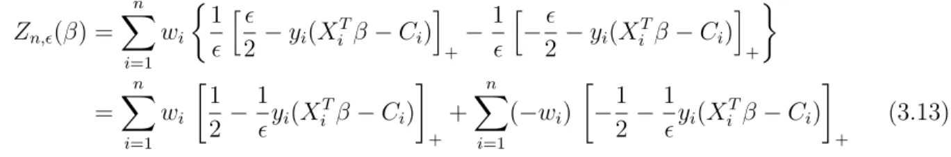
where >0 and [·]+ denotes the positive part of the argument. We illustrate the approxi-mation of a 0/1 loss by the difference between two hinge functions in Figure 3.8.

−3 −2 −1 0 1 2 3

0.0

1.0

2.0

3.0

y(X’β−C)

Loss

0/1 Loss Function

y(X’β−C)

Loss

− ε/2 0 ε/2 Convex part −1*Concave part Convex+Concave Approximation with ε

1

Figure 3.8: An illustration of using the difference between two hinge loss functions to approximate a 0/1 loss. A smaller provides a closer approximation.

To mitigate computational difficulties, we utilize the concave-convex procedure pro-posed by Yuille and Rangarajan (2003). The concave-convex procedure relies on

decom-posing an objective function, f(x), into a convex part,fconvex(x), and a concave part, fconcave(x) such that

f(x) =fconvex(x) +fconcave(x).

Optimization is carried out with an iterative procedure in whichfconcave(x)is linearized at the current solution x(t),

x(t+1) = arg min x

h

fconvex(x) + (x−x(t))f

0

(51)

making each iteration a convex optimization problem. The first value x(0) can be initial-ized with any reasonable guess.

To apply the concave-convex procedure to our optimization problem, we define the first term in Equation (3.13) as fconvex(β)and the second term as fconcave(β). The gradient of the concave part, fconcave(β), is

∂

∂βfconcave(β) =      Pn

i=1wi 1yiXi0

if 1 2 +

1 yi(X

T

i β−Ci)<0 0 if 1₂ +1yi(XiTβ−Ci)>0

Applying the concave-convex procedure to the above decomposition, we obtain

β(r+1) = arg min β ( _n X i=1 wi 1 2− 1

yi(X

T

i β−Ci)

+ + n X i=1 wi 1

yiX 0

i(β−β (r)₎_·_I

1 2+

1

yi(X

T i β

(r)₋_C i)<0

)

, (3.14)

where β(r) denotes the estimated β at therth iteration. The final form can be solved with

a standard convex optimization algorithm with a decreasing sequence of ={20_,₂−1_,_{· · · }}_. Specifically, the initial values for both the simulation studies and the real data example were generated using a coarse grid search. Given the initial value, we solve Equation (3.14) with = 20. The solution with _{= 2}0 is then used as the initial value to solve Equation (3.14) with = 2−1. This is repeated until the maximum relative change over all covari-ates is less than one percent. In this study, the fminsearch function from the optimization

toolbox in MATLAB was used to solve for β. The fminsearch function performs

(52)

3.2.3 Inference

The confidence intervals for parameter estimates are obtained using a subsampling method since the bootstrap does not consistently estimate the asymptotic distribution for estimators with cube-root convergence (Abrevaya and Huang 2005). The subsampling method described below is from Politis et al. (1999). Subsampling can produce consistent estimated sampling distributions under extremely week assumptions even when the boot-strap fails and it can be used to obtain confidence intervals for parameter estimates. It should not be used to obtain standard errors; however, since our estimators are not nor-mally distributed, even asymptotically (Section 3.3.3); therefore, there is no simple relation between the distribution of the estimators and standard errors (Horowitz 2010, page 108).

The justification for using the subsampling method in our study is discussed further in Section 3.3.3.

To obtain the confidence intervals of minimizer of Equation (3.13), _βˆ

n,, we produce subsamples K1, K2,· · · , KNn where Kj’s are the Nn ≡

n b

distinct subsets of {(Ci, Xi, δi)i=1,···,n} of size b. Let βτ denote the true parameter values and βˆn,,b,j denote the estimated value

produced by solving Equation (3.14) using the Kjth dataset.

Define

Ln,b(x) =Nn−1 Nn

X

j=1

I[b1/3( ˆβn,,b,j−βˆn,)≤x] and cn,b(γ) = inf{x:Ln,b(x)≥γ}.

From Theorem 2.2.1 of Politis et al. (1999), for any 0< γ <1, P h

n1/3( ˆβn,−βτ)≤cn,b(γ)

i

→

γ under the condition that b → ∞ asn → ∞ and b/n → 0. It follows that for any 0< α <0.5,

Phcn,b

α

2

< n1/3( ˆβn,−βτ)≤cn,b

1−α 2

i

(53)

thus an asymptotic 1−α level confidence interval for βτ can be constructed with

h

ˆ

βn,−n−1/3cn,b

1− α 2

, βˆn,−n−1/3cn,b

α

2

i .

Symmetric confidence intervals can be obtained by modifying the above approach slightly. Define

˜

Ln,b(x) =Nn−1 Nn

X

j=1

I[b1/3|βˆn,,b,j −βˆn,| ≤x] and c˜n,b(γ) = inf{x: ˜Ln,b(x)≥γ}.

Again , if b → ∞ as n → ∞ and at the same timeb/n → 0, a symmetric confidence interval for βτ can be constructed as

h

ˆ

βn,−n−1/3c˜n,b(1−α), βˆn,+n−1/3c˜n,b(1−α)

i

. (3.15)

Symmetric confidence intervals are desirable because they often have nicer properties than the nonsymmetric version in finite samples (Banerjee and Wellner 2005). This fact was also observed in our simulation studies; hence, symmetric confidence intervals are rec-ommended and used in this paper.

To avoid large scale computation issues, a stochastic approximation from Politis et al. (1999) is employed where B randomly chosen datasets from{1,2,· · · , Nn} are used in the above calculation. Furthermore, the block size is chosen using the method implemented in Delgado et al. (2001) and Banerjee and Wellner (2005). Briefly, the algorithm for choosing block size is described below.

Step 1: Fix a selection of reasonable block sizesb between limitsblow and bup. Step 2: Draw M bootstrap samples from the actual dataset.

(54)

within the mth interval based on block size b and zero otherwise.

Step 4: Compute ˆh(b) = M−1PM

m=1Rm,b.

Step 5: Find the value˜b that minimizes |ˆh(b)−α| and use˜b as the block size when

con-structing confidence interval for the original data.

3.3 Asymptotic Properties

3.3.1 Identifiability

Prior to deriving the asymptotic properties of the proposed estimator, we will discuss a set of sufficient conditions for identifiability.

For a fixed quantile τ, let

Zn(β) = 1

n

X

i=1

τ I(δi = 0)I(XiTβ−Ci ≤0) + (1−τ)I(δi = 1)I(XiTβ−Ci >0)

,

and

Z(β) = E[τ I(δ = 0)I(X0β−C ≤0) + (1−τ)I(δ = 1)I(X0β−C >0)].

Letβτ denote a minimizer of Z(·). The following conditions will be used in subsequent theorems.

Condition 1. The support of fX is not contained in any proper linear subspace of <k. Condition 2. For a fixed τ, with probability one, both the support of the conditional den-sity of C given X, fC|X(·), and the support of the conditional density of T given X, fT|X(·), contain XTβτ in their interiors.

Condition 1 is the typical full-rank condition.

(55)

mini-We prove Lemma 3.3.1 by showing Z(β)− Z(βτ) > 0, ∀β 6= βτ. A detailed proof is provided in Section 3.6. In our real data application, we suggest an empirical way to identify quantiles which are estimable.

3.3.2 Consistency

For a fixed quantile τ, let

Zn,(β) = n

X

i=1

τ I(δi = 0)

I(X_iTβ−Ci ≤ −

2) +I(|X T

i β−Ci|<

2) −1 (X T

i β−Ci−

2)

+(1−τ)I(δi = 1)

I(X0β−Ci >

2) +I(|X T

i β−Ci| ≤

2) 1 (X T

i β−Ci+

2)

We assume the following conditions for the consistency theorem.

Condition 3. Let β ∈ B where B is a compact subset of <k _{which contains} _β

τ as an inte-rior point.

Condition 4. MT ≡ supT ,X fT|X(T |X) <∞ and MC ≡ supC,X fC|X(C |X) <∞ where

fC|X and fT|X are the conditional density of C given X and T given X, respectively. Let_βˆ

n, be the minimizer of Zn,(·) inB.

Theorem 3.3.2. Under Conditions 1–4, βˆn, converges to βτ in probability as n → ∞ and

→0.

The proof follows by first showing that the collection of functions in Zn(β) is a VC-subgraph class and hence Zn(β) converge almost surely uniformly to Z(β). In addition,

Zn,(β) converges almost surely uniformly to Zn(β)as n → ∞and → 0; thus we can conclude that Zn,(β) converges almost surely uniformly to Z(β). Next, we prove thatZ(·) is continuous. Conditions 1 and 2 provide sufficient conditions for identifiability and hence,

(56)

that _βˆ

n, converges to βτ in probability by a standard argument for M-estimators (Theo-rem 2.1 of Newey and McFadden (1994)). A detailed proof is provided in Section 3.6.

3.3.3 Asymptotic Distribution

This section shows that n1/3_{( ˆ}_β

n,−βτ) converges to a nondegenerate distribution. The convergence rate is atypical because our objective function (3.12) is non-smooth and not everywhere differentiable; this is sometimes called the “sharp-edge effect” (Kim and Pollard 1990). We will make the following assumptions which guarantee the asymptotic distribu-tion will be nondegenerate, namely

Condition 5. The which is used in Equation (3.13) iso(n−2/3₎_.

Condition 6. The true distribution P of C, T and X is absolutely continuous with respect to Lebesgue measure.

Condition 7. X is bounded. Condition 8. Let V(βτ)i,j = Px

XiXjfC|X(X0βτ |X)fT|X(X0βτ |X)

and V(βτ) is posi-tive definite where Xi and Xj are elements of X.

We may now proceed with the main result. Theorem 3.3.3. Under Conditions 1–8, the process

n2/3Zn βτ +sn−1/3

−Zn(βτ)

:s∈ <k _{converges in distribution to a Gaussian} pro-cess

Γ(s) :s∈ <k _{with continuous sample paths, mean} _s0_V₍_β

τ)s/2, and covariance H, where V is the second order expansion of Z(β) at βτ, and

H(s, r) = lim

α→∞ αPC,X (

τ −FT|X(C |X)

2

I

X0r∨X0s

α < C−X 0

βτ ≤0

+I

0< C−X0βτ <

X0r∧X0s α

(57)

Theorem 2 follows by verifying the conditions of the main theorem from Kim and Pol-lard (1990). Provided that V is positive definite, we can conclude that n1/3( ˆβn,−βτ) con-verges to a nondegenerate distribution. A detailed proof is provided in Section 3.6.

Subsampling can produce consistent estimated sampling distributions for our estima-tor and it is an immediate consequence of Theorem 2.2.1 from Politis et al. (1999). In our study, we choose block size b = Nγ _where _γ ₌ _{₁_/₃_,₁_/₂_,₂_/₃_,₃_/₄_,₀_.₈_,₅_/₆_,₆_/₇_,₀_.₉_,₁₂_/₁₃_, 0.95} thus b → ∞ and b/N → 0as N → ∞. n1/3_{( ˆ}_β

n, −βτ)converges to a nondegenerate continuous distribution. All conditions in Theorem 2.2.1 from Politis et al. (1999) are met thus we can construct confidence intervals as stated in Section 3.2.3.

3.4 Numerical Studies

3.4.1 Simulation

Two simulation studies were carried out to test the finite sample performance of our es-timator. We used conditional quantile functions which were linear in the covariate for each studies. In the first scenario, Simulation 1, the conditional quantile functions had identi-cal linear coefficient and differed only in intercept. In the second scenario, Simulation 2, both the intercepts and covariate effects varied over the quantiles. Simulation 1 represents a situation where the errors are independent and identically distributed and Simulation 2 represents a situation where the errors are heteroscedastic.

In Simulation 1, the covariate is X ≡(1, X1, X2)0 where X1 ∼ Uniform [0,2]and X2 ∼ Bernoulli(0.5). The unobserved failure times, T, were generated from the linear model, T = 2 + 3X1 + X2 + 0.3U. The observation times, C, were generated from the lin-ear model, C = 1.9 + 3.2X1 + 0.8V when X2 = 0 and C = 3.1 + 2.8X1 + 0.8V when X2 = 1. Both U and V were generated from N(0,1). The proportion of events oc-curred prior to observation time, δ = 1, was about 50%. The underlying 0.25 quantile is