Optimizing the polarization
for a brighter CQED
Single Photon Source
THESIS
submitted in partial fulfillment of the requirements for the degree of
MASTER OF SCIENCE in
PHYSICS
Author : M.F. van de Stolpe
Student ID : s0000000
Supervisor : MSc. H.J. Snijders
Dr. W. L ¨offler Prof.dr. D. Bouwmeester 2ndcorrector : Prof.dr. M.P. van Exter
Optimizing the polarization
for a brighter CQED
Single Photon Source
M.F. van de Stolpe
Huygens-Kamerlingh Onnes Laboratory, Leiden University P.O. Box 9500, 2300 RA Leiden, The Netherlands
April 13, 2017
Abstract
Self-assembled InAs/GaAs quantum dots currently have the highest overall single photon source (SPS) performance, but one of the limiting factors for the brightness is the extraction of single
photons from the excitation laser pulse. Since the SPS is excited resonantly for maximal indistinguishability, a difference in polarization is used to extract the single photons from the incident
excitation laser light. In this work we studied ways to maximize the collection of single photons and the brightness of the SPS both
experimentally and theoretically. The system of a quantum dot in an optical cavity was simulated semi classically. Two new brighter
configurations for the input and output polarization were found, one through analytical analysis and one with an optimization algorithm. These two new polarization configurations were tested
in the lab along with the configuration that is conventionally used, which resulted in an SPS which wastwice(analytical analysis) andthreetimes (optimization algorithm) as bright as the
conventional configuration. We show that the brightness can be improved by another factor of three through optimizing one of the
Contents
1 Introduction 1
2 Theory and simulation 7
2.1 Semi-classical model 7
2.1.1 Formula 8
2.1.2 Limits 9
2.2 Parameters 9
2.3 Understanding the model 12
2.3.1 Quantum dot angle near 0◦ or 90◦ 12
2.3.2 Cavity mode splitting 15
2.4 Optimal polarization configuration 17
2.4.1 Polarization (lab adjustable parameter) 18
2.4.2 Sample dependent parameters 22
3 Materials and Methods 25
3.1 Materials 25
3.1.1 Experimental setup 25
3.1.2 Sample 26
3.2 Methods 27
3.2.1 Laser scan 27
3.2.2 Polarization scan 27
3.2.3 Voltage scan 28
3.2.4 g(2)(τ)-measurement 28
4 Experimental results and discussion 29
4.1 Sample dependent parameters 30
4.2 Laser scan line shapes 33
4.3.1 Single photons and brightness 36
4.3.2 Comparison 40
4.4 Mechanism behind brighter SPS 41
4.5 Discussion on the higher intensity 42
5 Conclusion 47
6 Outlook 49
Chapter
1
Introduction
The discovery of stimulated emission opened a whole new field of re-search culminating in a set of light sources with high performance, high reliability, yet low cost. These light sources (e.g. LASERs, LEDs) are now used for a broad range of applications in everyday life. The next step in this field of research will be to produce non-classical light sources. These sources are characterized by the ability to control their quantum fluctua-tions for which a single photon source serves as a mayor building block [1]. Moreover, these single photon sources are needed for most quantum information technologies [2–7] such as quantum key distribution [8, 9] or boson sampling [10].
Although there is still no ideal single photon source, a host of mate-rial systems has been researched for its ability to produce single photons on demand [1] and some of the more promising systems have been engi-neered to come close to the ideal single photon source. The question this might raise is therefore what such an ideal single photon source looks like. Aharonovich, Englund and Toth [1] describe the ideal single photon source as follows: “The ideal on-demand SPE (single photon emitter) emits exactly one photon at a time into a given spatiotemporal mode (high pu-rity), and all photons are identical so that if any two are sent through sep-arate arms of a beam-splitter, they produce full interference (a signature of indistinguishability).” But the demands on the source are even higher as for most applications the ideal single photon source also has to be sta-ble, bright, and fast. Here, stable means that the source does not blink or bleach, the brightness is the maximum rate at which single photons can be emitted (or collected), and fast means that the source has a short lived excited state.
pho-ton source, however, are still the single phopho-ton purity and the indistin-guishability. The single photon purity of the source is quantified by the dip in the intensity correlation function g(2)(τ) at zero time delay which
quantifies the probability to have two photons at the same time (atτ =0).
The indistinguishability is quantified by a dip in the Hong-Ou-Mandel two-photon interference experiment which measures the destructive inter-ference of two photons that arrive simultaneously at a 50:50 beam splitter. Currently, self-assembled InAs/GaAs quantum dots perform the best overall as they are the only material system that shows single photon pu-rities larger than 99% (g(2)(0) < 0.01) [11–14] and indistinguishability of the produced single photons of more than 90% [11, 14]. Most other mate-rial systems show increased multi photon emission with purities around 70%-90% [1].
Possibly the biggest advantage of quantum dots, however, is that they are atom-like emitters in a solid state host. This allows the quantum dot to combine the optical properties of atoms with the scalability and conve-nience of solid state systems [11, 15]. Moreover, quantum dots can be in-corporated in optical micro cavities which increase the spontaneous emis-sion rate due to the Purcell effect, making them a very attractive system for a fast single photon source [2].
The system we are working with is such a quantum dot coupled to an optical cavity. This is thus a system with a possible purity of>99% under resonant excitation and a possible indistinguishability of>90%. Further-more it is stable due to the solid state environment and fast due to Pur-cell enhanced spontaneous emission. This conforms to the statement that these systems have the best all-round performance currently available[16– 19].
There is one aspect of the ideal single photon source, however, that we did not yet mention: the brightness. We defined it earlier as “the maximal rate at which single photons can be emitted (or collected)”. The emission rate, however, is related to the lifetime of the excited state. Therefore, for a specific single emitter system, the ”brightness” can only be affected by the extraction efficiencyof single photons from the emitter. This brightness is of particular interest in this thesis: can we improve the brightness of a cavity quantum electrodynamics single photon source (a quantum dot emitter in an optical cavity) through optimizing the configuration of the input and output polarizer?
indistinguishabil-3
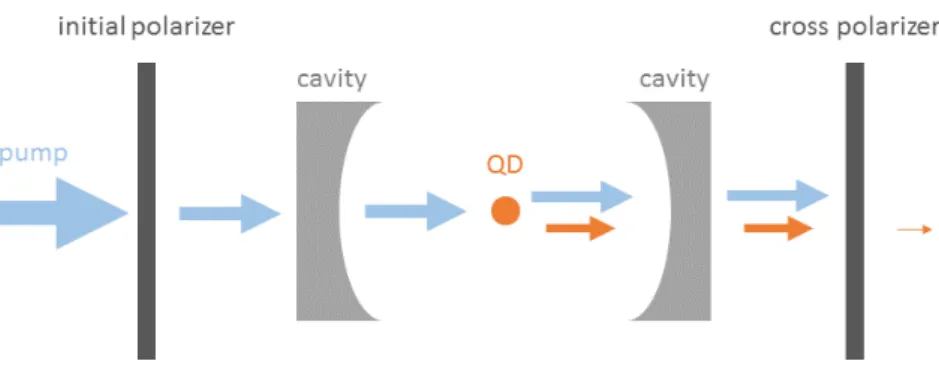
Figure 1.1: Schematic representation of the cavity with the quantum dot, the po-larizers, and the pump (blue) and quantum dot (orange) light. Part of the light emitted by the quantum dot is filtered out by the cross polarizer, resulting in a lower transmitted than emitted single photon intensity. A brighter single photon source can be created by optimizing the polarization configuration to allow more light emitted by the quantum dot to pass through the cross polarizer while still blocking all laser light needed for the excitation of the quantum dot.
ity. With resonant excitation there are no additional relaxation processes from higher excited states necessary before the photon is emitted. This is difficult to implement practically since the single photons have to be sep-arated from the strong excitation laser pulse [2]. One way to separate the two is by using a difference in the polarization of the light (figure 1.1). A further reason to use polarization to filter the single photons from the ex-citation laser pulse lies in the nature of the system used: a polarization non-degenerate quantum dot in a polarization non-degenerate cavity. A polarization non-degenerate system is a system with two modes that are split spectrally and have orthogonal linear polarization (figure 1.2), thus both the quantum dot and the cavity have two spectrally split modes with orthogonal polarization.
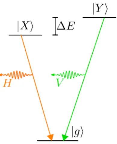
Figure 1.2: Schematic representation of the polarization non-degenerate modes of the quantum dot. The quantum dot has an X and an Y mode, separated in energy by∆E(split spectrally by the quantum dot splitting). The X mode emits horizontally polarized light and the Y mode vertically polarized light. Figure adapted from Lodahl, Mahmoodian, and Stobbe [4].
extracted because the quantum dot emits light in a different polarization (the quantum dot dipole changes the polarization of the scattered light). So how much of the emitted single photons can be extracted and collected after the output polarizer?
The output polarizer is aligned with the empty cavity mode polariza-tion (i.e. without the excitapolariza-tion laser light). Therefore, the quantum dot has to emit its single photon in this empty cavity mode polarization for it to be collected. But how can the quantum dot emit in that cavity mode polarization if it is excited from the other cavity mode polarization? The polarization of the quantum dot modes is not necessarily aligned with the cavity mode polarizations. Therefore, when a quantum dot mode is ex-cited by the excitation laser light in one cavity mode polarization, it can emit a single photon in the other cavity mode with the orthogonal polar-ization and this single photon can then be collected.
5
only 0.5 since that goes ascos(θQD). For a high-brightness single photon source, a strong coupling of the polarization of the quantum dot mode to the polarization of the cavity mode is preferred and therefore a small quantum dot angle. This in turn, however, also means that the single photons emitted by the quantum dot are much more likely to be emitted in polarization of the cavity mode already filled with the excitation laser light since it goes as cos2(θQD) (but is possibly even higher due to stim-ulated emission in that cavity mode). The photons emitted in this filled cavity mode polarization, however, cannot be filtered from the excitation laser light and thus cannot be collected as single photons. Therefore, even though the coupling between the polarization of the quantum dot mode and the polarization of the cavity mode is strong, a small quantum dot an-gle should also result in a low brightness of the sinan-gle photon source since all light in the filled cavity mode polarization is blocked by the output polarizer.
Chapter
2
Theory and simulation
We want to fabricate a single photon source and therefore use a quantum dot in a cavity. We use an input and output polarizer in cross polarization to filter out the single photons from the excitation laser light. However, the output polarizer inherently also blocks some single photons. Therefore we want to optimize the polarization configuration in order to produce a brighter (better) single photon source.
The parameter space of the polarization configuration is so large, that it is not doable to try to optimize the polarization configuration directly in the lab. We will first study the system of a polarization non-degenerate quantum dot in a polarization non-degenerate cavity numerically in the semi classical approximation to find out if a better polarization configu-ration exists. We will define the optimal configuconfigu-ration as a configuconfigu-ration where, for a certain laser frequency, the intensity without the quantum dot is practically zero, while the intensity with the quantum dot is high. For this definition, there exist more optimal polarization configurations and we will try two of these configurations in the lab in chapter 4.
2.1
Semi-classical model
2.1.1
Formula
There are multiple formulas for the description of a quantum dot in a cav-ity, all with their own notation and choice of variables. For the simulation we will go with the formula from the thesis of Morten P. Bakker [20–23]:
t =ηout 1
1−i∆+1−2Ci∆0
(2.1)
withtthe transmission,ηoutthe output coupling efficiency,∆ =2(ωlaser−
ωcavity)/κthe dimensionless relative detuning between the laser and the cavity (with a factor 2/κ),∆0 = (ωlaser−ωQD)/γ⊥the dimensionless
rela-tive detuning between the laser and the quantum dot (with a factor 1/γ⊥),
and 2C = g2×2/κ×1/γ⊥ the device cooperativity with g the quantum
dot mode coupling strength, κ the total intensity damping of the cavity
andγ⊥the quantum dot dephasing rate.
This formula depends thus on the four intrinsic sample parameters:
ηout, 2/κ, 1/γ⊥, and g2 and on the two resonance frequenciesωcavity and
ωQD of the cavity and the quantum dot, all of which we can find from experiments.
This formula, however, does not yet take the polarization non-degeneracy of the quantum dot and the cavity into account. To incorporate the polar-ization we replace the scalars with 2x2 matrices. We assume equal reflec-tion and transmission coefficients for the two cavity mode polarizareflec-tions as well as equal decay rates. The line width of the quantum dot modes is assumed equal as well, so that the difference between both the cavity and the quantum dot modes is given solely by their resonance frequency. We rewrite the formula above with 2x2 matrices and with the division becom-ing a matrix inversion:
t2x2 =ηout I2x2−
i∆H 0 0 i∆V
+R−θQD
2C
1−i∆0X 0 0 1−2iC∆0
Y !
RθQD !−1
(2.2) witht2x2denoting the 2x2 transmission matrix, I the identity matrix, and A−1a 2x2 matrix inversion of matrixA. Furthermore,∆H(V) is the
dimen-sionless relative detuning between the laser and the horizontally (verti-cally) polarized cavity mode (still with a factor 2/κ),∆0X(Y) the
dimension-less relative detuning between the laser and the X(Y)-quantum dot mode
(still with a factor 1/γ⊥) andRθ =
cos(θ) −sin(θ)
sin(θ) cos(θ)
the rotation
ma-trix for an angleθ, to incorporate the rotation of the quantum dot system
2.2 Parameters 9
This adjusted formula effectively adds only one extra factor which is the angle θQD between the cavity frame and the quantum dot frame. Al-though this angle might not seem to be very interesting, we will find that it has a mayor influence on the possible quality of the single photon source and we will therefore discuss its importance in sections 2.3.1 and 2.4.2.
2.1.2
Limits
The semi classical model breaks down due to saturation. This saturation is governed by a dimensionless parameters given in the paper by Armen and Mabuchi [24]. The critical photon number is a measure for the amount of photons needed to saturate the response of the quantum dot:
n0 =
γkγ⊥
4g2 (2.3)
with γk the dissipative relaxation rate in modes other than the preferred
cavity mode and γ⊥ = γk/2+γnr the quantum dot dephasing rate and g2the quantum dot mode coupling strength. These rates and the coupling strength depend on the specific system and saturation of the quantum dot is reached for n0 < 1. For the quantum dot in the cavity, the simulation holds thus for very low photon numbers in the cavity only. This means that we will need a very low power of the exciting laser light in order to not saturate the quantum dot.
2.2
Parameters
Some of the parameters used in the simulation have been addressed briefly in the previous section: the two frequencies of the cavity modes, the two frequencies of the quantum dot modes and the quantum dot angle. We will not refer any further to the intrinsic sample parameters (ηout, 2/κ,
1/γ⊥, and g2) in this thesis and focus solely on the three sample
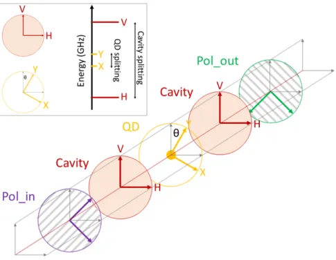
Figure 2.1: Schematic of the components and angles used in the semi classical simulation of a quantum dot in a cavity. The orthogonal polarizations of the cavity modes double as the axes of the reference frame. The polarization angle is defined as the angle the polarizers make with respect to the cavity axes (reference frame). The modes of the cavity (quantum dot), labeled by H (X) and V (Y), are orthogonal in polarization and spectrally separated by the cavity (QD) splitting. By convention, the energies of the cavity (quantum dot) modes is defined such that the V (Y) mode has a higher energy than the H (X) mode. The quantum dot system is rotated by an angleθQD with respect to the cavity axes (reference
2.2 Parameters 11
A schematic of the components and angles used in the semi classical simulation of the polarization non-degenerate quantum dot in the polar-ization non-degenerate cavity is shown in figure 2.1. As can be seen from equation 2.2, the cavity axes are used as the reference frame for the po-larization. The center between the frequency of the two cavity modes is therefore also defined to be 0 GHz and thus our reference laser frequency. Furthermore, the X mode of the cavity is defined to be lower in energy than the Y mode and similarly is the H mode of the quantum dot defined to be lower in energy than the V mode.
The list of tunable parameters used in the simulation is split in a part for the quantum dot in the cavity system and a part for the polarization. The first consists of 6 parameters and the latter of 5:
• flaser:
the laser frequency relative to the center of the two cavity modes. The center between the two cavity modes is defined as 0 GHz and thus our reference laser frequency.
• cavsplit:
the frequency difference between the two cavity modes.
• QDsplit:
the frequency difference between the two quantum dot modes.
• QDdetuning:
the frequency of the center between the two quantum dot modes relative to the center between the two cavity modes.
• thetaQD:
the angle between the cavity frame and the quantum dot frame.
• withQD:
a Boolean that determines whether we compute the transmission with or without a quantum dot present in the cavity. This allows us to determine the so called quantum dot contrast: the difference in transmitted intensity with and without a quantum dot present.
• polina, polinb, polouta, poloutb:
two scalars per polarization to store the input polarization ein~ and the output polarizationeout. The formula used is given by:~
~
ein =
1 p
1+polina2+polinb2
1
polina+i·polinb
• withpolout:
a Boolean that determines whether we compute the transmission with or without an output polarizer present. This allows us to simu-late the total transmission which is useful to compare to polarization scan experiments.
Some of these parameters are adjustable in the lab while others are sample dependent. We can changeflaserwith the scanning laser,QDdetuning
and withQD through the bias voltage on the PIN junction, and of course the 5 polarization parameters. The three sample dependent parameters,
cavsplit, QDsplit, andthetaQD, can be found through analysis of a po-larization scan of the sample.
2.3
Understanding the model
Now that we have found a way to simulate the behavior of the quantum dot in the cavity as a function of the input and output polarizers, we will elaborate some more on two of the sample dependent parameters: the quantum dot angle and the cavity splitting. First we will look at the quan-tum dot angle and see that it has a profound effect on the brightness of the single photon source and that the angle has a 180◦ rather than a 90◦ rotational symmetry. Secondly we will see that the cavity splitting plays a major role in the polarization of the transmitted light through the cavity due to birefringence induced by the spectrally split cavity modes.
2.3.1
Quantum dot angle near 0
◦or 90
◦At first sight, a quantum dot angle of θQD= 0◦ or θQD= 90◦ should not
make a difference since the cavity mode polarizations and quantum dot mode polarizations overlap in either case. There is a subtle difference, however, which comes from the non-degeneracy of the cavity and quan-tum dot mode polarizations. AroundθQD= 0◦, the X mode of the quantum dot interacts with the H mode of the cavity (by definition of the quantum dot angle, see figure 2.1) while forθQD= 90◦, the X mode of the quantum
2.3 Understanding the model 13
high energy quantum dot mode with the high energy cavity mode. In con-trast, aroundθQD= 90◦the low energy quantum dot mode interacts mainly
with the high energy cavity mode and vice versa for the high energy quan-tum dot mode. Although this might seem like a trivial difference, it turns out to greatly affect the maximal brightness of a single photon source in such a system.
The total transmission due to the polarization non-degenerate quan-tum dot is enhanced for a quanquan-tum dot splitting up to about 4 GHz when the quantum dot angle is nearθQD= 0◦and reduced when the angle is near
θQD= 90◦. This is due to the effect the quantum dot has on the phase of
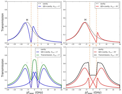
the light in the cavity. The quantum dot effectively adds a phase to the light with which it interacts, thus causing light of a different frequency to fit more optimally in the cavity mode. This is illustrated in figure 2.2. The cavity mode is shown in grey dashes and the cavity mode with a quan-tum dot in the cavity is shown in red. A dip is visible at the frequency of the quantum dot mode since the light is absorbed by the quantum dot mode at that frequency. A Fano like peak is visible at a slightly higher frequency (for the lower energy cavity mode): the light picks up a phase from the quantum dot which causes the light at that frequency to fit more optimally in the cavity than without the quantum dot present.
If we think of the effect the quantum dot mode has on the cavity mode as if it pushes part of the light in the cavity mode spectrally outward, we can understand the difference between a quantum dot angle of θQD= 0◦
andθQD= 90◦more easily. Recall that the X and the H mode are defined to be lower in frequency (energy) than the Y and V modes. AroundθQD= 0◦,
the Fano like peaks are pushed towards each other resulting in a peak (fig-ure 2.2 left). Around θQD= 90◦, however, the Fano like peaks are pushed away from each other resulting in a relative dip (figure 2.2 right).
Based on the above results, we would like our sample to have a quan-tum dot angle aroundθQD= 0◦ for a bright single photon source. We will see that this is partly true as the optimal quantum dot angle lies between
θQD= 5◦ and θQD= 50◦ for low quantum dot splitting which is definitely
Figure 2.2:Simulation of the system with the quantum dot angle atθQD=0◦(left)
and atθQD=90◦(right). The input polarizer is set toθpol=45◦(both cavity modes are excited equally) for all plots. The output polarizer is set to different settings for the different plots. (top): the output polarizer is set toθpol=0◦. (bottom, blue
and red curves): the output polarizer is set to θpol= 0◦ andθpol= 90◦. (bottom, green and black curves): no output polarizer is used. ForθQD=0◦(left), the H (V)
mode of the cavity interacts with the X (Y) mode of the quantum dot (top) and the Fano like line shapes created by the quantum dot overlap resulting in a peak in total transmission (bottom). ForθQD=90◦(right), the H (V) mode of the cavity
2.3 Understanding the model 15
2.3.2
Cavity mode splitting
The goal of the output polarizer is to stop the coherent excitation laser light from being transmitted (or all light when no quantum dot mode is present in the cavity). Therefore, to find a possibly more optimal configuration, we decided to look into the polarization of the light coming out of the cavity. This polarization depends mainly on two parameters: the polarization of the incoming light and the cavity splitting (how much the cavity modes are split spectrally).
Firstly we looked at horizontal and vertical input polarization. For horizontal input polarization, only horizontal polarized light will exit the cavity because it will only interact with the horizontally polarized cavity mode. The polarization does thus not depend on the cavity splitting and the same story holds for vertically polarized light. This is why a polariza-tion configurapolariza-tion with a horizontal linear input polarizer and a vertical linear output polarizer blocks the excitation laser light. We will refer to his polarization configuration as 90Cross since the linear input and output polarizers are cross polarized at an angle of 90◦to each other.
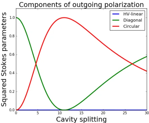
The second logical input polarization is for an input polarization ex-actly between the polarizations of the cavity modes: a linear polarizer at 45◦ to the H or V mode of the cavity. For this input polarization, the po-larization of the light coming out of the cavity does depend on the cavity splitting (figure 2.3).
At a cavity splitting of 0 GHz, the cavity is polarization degenerate and thus does not change the polarization of the incoming light. At higher cavity splitting, however, the cavity becomes birefringent due to the fre-quency mismatch between the horizontally and vertically polarized cavity modes. This birefringence causes the diagonally polarized light to pick up a circular component. The light exiting the cavity is nearly circular around a cavity splitting of 11 GHz for the parameters of our samples and scales with the total intensity damping factor of the cavity κ. The samples in
the lab have a cavity splitting of around 10 GHz and the outgoing polar-ization is thus still pretty close to circular for an incoming polarpolar-ization of 45◦. When simulated, this polarization configuration showed a higher intensity with the quantum dot present than the 90Cross polarization con-figuration. This 45◦ in, circular out polarization configuration apparently blocks less of the single photons emitted by the quantum dot while it is still a configuration that should be relatively easy to reproduce in the lab. We will refer to this polarization configuration as45Circ.
2.4 Optimal polarization configuration 17
configuration (90Cross). This also means that there is probably an even better polarization configuration possible. That configuration, however, will most likely have a polarization of elliptical nature which makes it dif-ficult to find solely through manual analysis of the simulation results. In order to find such a configuration, we will therefore run an optimization algorithm over the set of parameters that we can tune in the lab.
2.4
Optimal polarization configuration
The standard polarization configuration with two crossed linear polariz-ers (90Cross) apparently blocks some of the single photons generated by the quantum dot. There is another polarization configuration (45Circ) that also blocks the excitation laser light, but allows more light emitted by the quantum dot to pass through the output polarizer. This strengthens our belief that an even more optimal polarization configuration can be found. We will thus run an optimization algorithm over the lab adjustable pa-rameters (polarization configuration, detuning of the quantum dot, and laser frequency), for the range of parameters set by the sample (cavity splitting, quantum dot splitting, and quantum dot angle). As stated pre-viously, the optimal configuration is a configuration where, for a certain laser frequency, the intensity without the quantum dot is practically zero, while the intensity with the quantum dot is high. Based on this definition, we used an adjusted visibility as the valuation function:
valuation= IwithQD−(InoQD+offset)
IwithQD+ (InoQD+offset)
(2.5)
with IwithQDthe transmitted intensity with a quantum dot present, InoQDthe
transmitted intensity without a quantum dot present, andoffsetan offset to the intensity without a quantum dot. The offset is added because the visibility is maximal when the intensity without a quantum dot is zero, while that does not necessarily result in a bright single photon source.
shows a definite trend as a function of the parameters set by the sample and therefore we can easily discern between points where a local mini-mum was found and points where the global minimini-mum was found. We will therefore ignore the erroneous pixels where a local minimum was found in the plots shown below (figures 2.4 - 2.7).
As stated above, the optimization algorithm searches the set of lab ad-justable parameters for a configuration where the intensity with the quan-tum dot is highest while the intensity without the quanquan-tum dot is prac-tically zero. The algorithm then returns the values for the intensity with and without a quantum dot, but it also gives the set of lab adjustable pa-rameters for those intensities.
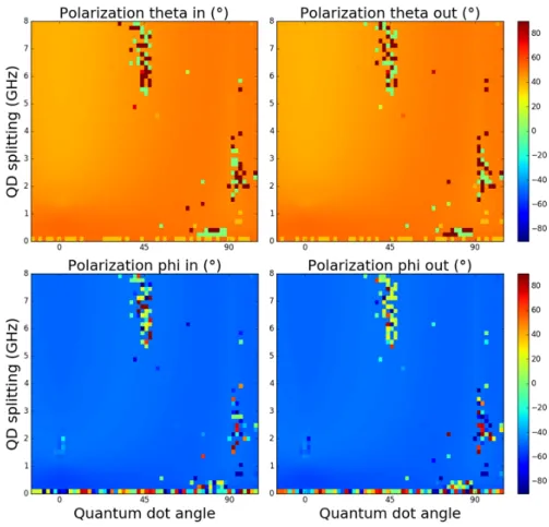
Although the total transmitted intensity as a function of the parame-ters set by the sample is interesting, we cannot change these parameparame-ters in the lab. We will therefore first look into the input and output polarization as a function of these parameters, since this thesis focuses on optimizing the polarization configuration. We will see that the input and output po-larization is identical apart from a complex conjugation. Furthermore, the polarization configuration does not depend on the quantum dot splitting or on the quantum dot angle and that only the phase between the horizon-tal and vertical polarization depends on the cavity splitting.
After we have analyzed the optimal polarization configuration, we will look at the optimal sample dependent parameters (cavity splitting, quan-tum dot splitting, and quanquan-tum dot angle). We will see that an optimal sample would have a cavity splitting of 5-15 GHz, a quantum dot splitting larger than 1 GHz and a quantum dot angle ofθQD= 20◦-60◦.
The above only holds, however, if the polarization configuration found by the optimization algorithm does indeed produce better results than the conventional polarization configuration for the sample in the lab. This sample lies somewhere in the three dimensional space of sample depen-dent parameters (cavity splitting, quantum dot splitting, and quantum dot angle), and if the optimal polarization configuration yields a brighter sin-gle photon source there, it should do so over the whole range of sample dependent parameters since the polarization configuration is nearly iden-tical through this three dimensional space.
2.4.1
Polarization (lab adjustable parameter)
oth-2.4 Optimal polarization configuration 19
erwise find non-physical optimal solutions in the rounding off error of the sin or cosine. In order to return to a more intuitive set of parameters, the polarization was reparameterized into two different scalarsθ andφvia:
~
ein =
sinθ
cosθeiφ
(2.6)
where θ determines factor of horizontally and vertically polarized light
and φ the phase between them. To get a feeling of how this
parameter-ization of the polarparameter-ization works, we will give some examples. For hor-izontally or vertically polarized light (θ = 0◦ or 90◦) φis undefined,
be-cause it describes an irrelevant global phase. For diagonally polarized lightθ =45◦and φ=0◦, and finally, for circularly polarized lightθ =45◦
andφ=90◦.
As we can see from figure 2.4, the optimal polarization configuration is almost completely independent of two of the three parameters set by the sample: the quantum dot splitting and the quantum dot angle. Further-more, the input and output polarization seem to be identical. The simu-lation, however, does still take the complex conjugate of the output po-larization, so the input and output polarization are actually each other’s complex conjugate. This shows up, however, only in the phase between the horizontally and vertically polarized light: the phase is identical but opposite in sign for the input and the output polarization.
As we can see from figure 2.5, the optimal polarization configuration does depend on the cavity splitting of the sample, but it does so only in the phase factorφand not in the factor of horizontally and vertically polarized
lightθ. This factor of horizontally and vertically polarized light is more or
less equal (θ ≈ 45◦) for all parameters set by the sample. Since this
2.4 Optimal polarization configuration 21
2.4.2
Sample dependent parameters
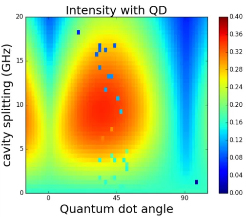
As stated above, the simulation returns the maximal intensity with the quantum dot for a certain polarization configuration with practically zero intensity (order 1E-5 for the optimal configuration) without a quantum dot in the cavity. We can look at this intensity with the quantum dot as the maximal possible brightness of the single photon source. This inten-sity is plotted as a function of the three sample dependent parameters in figures 2.6 and 2.7: cavity splitting, quantum dot splitting, and quantum dot angle.
We find from these figures that the maximal intensity is limited to about 0.4 on a scale of 0 toηout(the output coupling efficiency). (The inten-sity of a single cavity mode is 1 on this scale when the input polarization is aligned with this mode and no output polarizer is used (or if the output polarizer is aligned to that cavity mode polarization as well).) This is thus an upper limit to the brightness of the single photon source if we want to resonantly excite the quantum dot and thus use a polarizer to filter the excitation laser light.
2.4 Optimal polarization configuration 23
Chapter
3
Materials and Methods
3.1
Materials
Both the setup and the sample are very intricate and complicated, but we will describe both without much detail in this chapter and focus on the aspects important for this thesis only. For more info on the setup and the sample we refer to the thesis of M.P. Bakker [20] or the more recent paper by Snijders et al. [25].
3.1.1
Experimental setup
Figure 3.1: Schematic of the measurement setup. The sample with the quantum dot is located in the cold finger cryostat. The frequency of the scanning laser is locked to a Fabry-Perot. The output polarizer is in cross polarization with the input polarizer to filter out the incoming laser light. The single photon counters are connected to a coincidence counter that generates the intensity correlation functiong(2)(τ).
3.1.2
Sample
3.2 Methods 27
Figure 3.2: Schematic (left) and SEM image (right) of the sample with the cavity and quantum dots. The cavity consists of two multi layer thin film mirrors below and on top of the quantum dots. An oxide aperture is used for transverse confine-ment of the cavity mode. A PIN junction is used to tune the excitation frequency of the band structure of the quantum dot around the resonance frequency of the cavity. Trenches are etched in the sample to confine the light in the z-direction of the cavity.
3.2
Methods
The setup allows for a large set of measurements, but we will describe only the methods of the four measurements used in this thesis. Three of these depend on the ability of the laser to scan over a range of frequencies while the last needs a stable laser frequency.
3.2.1
Laser scan
The frequency of the scanning laser is swept over the scan range (about 80 GHz) while one of the APDs records the photons collected at each fre-quency. The result is a plot of the transmission intensity (in counts per second, cps) as a function of the relative laser frequency (in GHz).
3.2.2
Polarization scan
excited and a polarization scan allows us thus (among others) to find the axes of the cavity frame.
3.2.3
Voltage scan
The bias voltage over the PIN junction is swept over the scan range (about 0.2 V) and a laser scan is performed for each voltage in the scan range. This is used to shift the quantum dot energy by the quantum confined Stark ef-fect. The result is a 2D plot of the transmission intensity (cps) as a function of relative laser frequency (GHz) and applied bias voltage (V). The bias voltage changes the excitation frequency of the quantum dot and a volt-age scan allows us thus to find the voltvolt-age needed to tune the quantum dot frequency to the cavity frequency.
3.2.4
g
(2)(
τ
)-measurement
For photon correlation measurements, the frequency of the scanning laser is stabilized by locking it to a stable Fabry-Perot cavity. One of the APDs starts a time measurement as soon as a photon is detected while the other APD stops this measurement. This is a Hanbury-Brown and Twiss setup. The histogram of time delays between a photon detected at the start APD and the stop APD gives the temporal distribution of consecutive photon detection events. The probability to detect not the next, but any photon after a certain time is then given by the probability that this photon is the next one, plus the probability that this photon is the second one, plus etc. This probability distribution is related to the intensity correlation func-tiong(2)(τ)byP(τ) =hI(τ)ig(2)(τ). A single photon source is
character-ized by photon anti-bunching which shows up in the intensity correlation function as g(2)(0) < 1 and ag(2)(τ) measurement allows us therefore to
Chapter
4
Experimental results and
discussion
The goal of this thesis is to see whether we can improve the brightness of a cavity quantum electrodynamics single photon source through the optimization of the polarization configuration of the input and output po-larizer. The simulation showed that there is a better polarization config-uration possible than the conventionally used crossed linear polarizers (90Cross). This conventional polarization configuration is very easy to find in the lab while the optimal configuration as proposed by the opti-mization could be rather difficult to find since it is elliptical. The output polarization can be found experimentally by minimizing the transmission without a quantum dot. The elliptical input polarization is more difficult. As an alternative, we will therefore also look at the configuration that we found through analysis of the simulation results: 45◦ linear input polar-ization and circular/elliptical out (45Circ). The input polarpolar-ization is easy to find because it is linear and exactly between the H and V polarized modes of the cavity. The configuration of the output polarizer can then be found experimentally by minimizing the transmitted intensity without a quantum dot.
polar-izations and reproduce those in the lab. Finally, in order to characterize the quality of the single photon source, we will measure the photon char-acteristics through ag(2)(τ)measurement.
4.1
Sample dependent parameters
We can find the sample dependent parameters from a polarization scan (figure 4.1). The linear input polarizer is rotated over 180◦ with no output polarizer while a laser scan is performed at each frequency. This results in a 2D plot of the transmitted intensity as a function of relative laser fre-quency and input polarization angle. The two cavity modes will show up as large peaks and the quantum dot modes as small dips in those peaks. The cavity and quantum dot splitting can be found from the difference in relative laser frequency between the modes (that are separated 90◦ in input polarization angle). The quantum dot angle can be retrieved from the difference in angle of the maximum of the cavity mode peak and the minimum of the quantum dot dip.
From the polarization scan we extract a cavity splitting of about 10 GHz with a quantum dot splitting of about 2 GHz. To find the quantum dot angle, we fitted the peak of the cavity mode and dip of the quantum dot mode as a function of polarization angle with a Gaussian. The difference between the peak of the cavity mode and the dip of the quantum dot mode was found to be about 4◦. As described in section 2.3.1 there is a definite difference between θQD= 0◦ and θQD= 90◦. Therefore, to find the actual
4.1 Sample dependent parameters 31
Figure 4.1:A measurement of the transmitted intensity without an output polar-izer as a function of incoming polarization angle and laser frequency (arbitrary offset) with a quantum dot in the cavity. The inset shows the transmitted inten-sity as a function of incoming polarization angle for a laser frequency set to one of the cavity mode (red) and one of the quantum dot mode frequencies (black). The fit of these curves shows a relative angle difference between the two peaks of
4.2 Laser scan line shapes 33
4.2
Laser scan line shapes
As a tool to find the desired polarization configurations in the lab, we can simulate the shape of the laser scan for each configuration. This is most helpful for the optimal polarization configuration, but it will help to find the other two polarization configurations (45Circ and 90Cross) as well.
To recap, there are three polarization configurations that we would like to test in the lab for their brightness and quality of the single photon source. The first polarization configuration is the commonly used config-uration with two crossed linear polarizers aligned with the cavity mode polarizations that we will refer to as 90Cross. The second configuration is a linear polarizer under 45◦ to the cavity mode polarizations with an output polarizer which is nearly circular which we will refer to as45Circ. The third configuration is the configuration found by the optimization al-gorithm and consists of an elliptical in and reverse elliptical out which we will refer to asOptimal.
To reproduce the polarization configurations, we simulated four line shapes per configuration: two with and two without an output polarizer and both with and without a quantum dot present in the cavity. The line shapes without the output polarizer serve as a guideline for the input po-larization and the two with the output polarizer serve to confirm that we have found the desired polarization configuration.
4.2 Laser scan line shapes 35
4.3
Single photon source quality
The simulation along with the experimental results tell us that, if we are in-deed looking at single photons only in all three configurations, the bright-ness of the Optimal configuration is three times the intensity of the con-ventionally used 90Cross configuration (30x for the simulation) and that the 45Circ configuration is also already twice as bright (20x for the simu-lation). We do not yet know however if the intensity we see in the laser scans consists of single photons only. Therefore we will measure the in-tensity correlation function g(2)(τ) for different laser powers to analyze
the quality of the single photon sources for the three different polarization configurations.
4.3.1
Single photons and brightness
Although, as said, the intensity of the optimal configuration is three times as high as for the 90Cross configuration, we do not yet know if this inten-sity consists of single photons only. As stated briefly in methods, ag(2)(τ)
(intensity correlation function) measurement allows us to find out if we are looking at single photons since a single photon source is characterized by anti-bunching. This anti-bunching shows up in the intensity correla-tion funccorrela-tion as a dip atτ =0 since a single photon cannot be detected by
the two detectors at the same time (delay time between the detectors of 0). This behavior is purely quantum (since photons are inherently quantized) and cannot be explained classically.
For all three polarization configurations, the intensity correlation func-tion shows a clear dip atτ =0 up to 50% (figure 4.5), thus confirming that
we are looking at single photons in all three configurations. In order to compare the single photon brightness of the three polarization configura-tions, however, we will measureg(2)(τ)for different excitation laser
pow-ers. This enables us to see the saturation of the quantum dot as a decrease of the dip at τ =0. The decrease of this dip should overlap for the three
polarization configurations because it depends only on the quantum dot used and not on the polarization configuration.
This decrease of the dip (corresponding to an increase ofg(2)(0)) does indeed overlap for the three polarization configurations as a function of excitation laser power (figure 4.6), thus confirming that we are indeed looking at the saturation of the quantum dot in all three configurations. For each g(2)(τ) measurement, however, the amount of single counts
4.3 Single photon source quality 37
4.3 Single photon source quality 39
Figure 4.7:Fitted height of the dip in the measured intensity correlation function g(2)(τ) as a function of single counts for the three polarization configurations: 90Cross, 45Circ, and Optimal. The dashed parallel lines are added as a guide to the eye to show that the dip height starts to diminish at different count rates for the different polarization configurations.
is plotted as a function of single counts (figure 4.7), the points of the three polarization configurations do not overlap anymore: the dip starts to sat-urate at a different value of single counts for the three polarization config-urations.
Figure 4.8: Single counts as a function of laser power for the three polarization configurations: 90Cross, 45Circ, and Optimal along with lines with a slope of 1x, 2x and 3x the fitted slope for the data points up to 2 nW of the 90Cross configu-ration.
4.3.2
Comparison
The 45Circ configuration generates twice the amount of single counts recorded in the 90Cross configuration where Optimal generates three times this amount (for the same laser power up to the saturation laser power of about 5 nW). This means that the optimal configuration yields a 3x brighter sin-gle photon source.
4.4 Mechanism behind brighter SPS 41
Figure 4.9: Schematic representation of the cavity with the quantum dot, the po-larizers, and the pump (blue) and quantum dot (orange) light. Part of the light emitted by the quantum dot is filtered out by the cross polarizer, resulting in a lower transmitted intensity and coincidence count for the same excitation laser power. A brighter single photon source can be created by optimizing the po-larization configuration to allow more light emitted by the quantum dot to pass through the cross polarizer while still blocking the laser light needed for excita-tion.
4.4
Mechanism behind brighter SPS
In a very simplified approach, we can understand the mechanism of how the brightness of a single photon source depends on the polarization con-figuration. Let us assume that the polarization of the incoming laser light does not influence the excitation rate of the quantum dot or the polariza-tion of the light emitted by the quantum dot. The input polarizer sets the polarization of the light in the system (initial polarizer) and the output po-larizer fully blocks this excitation light (cross popo-larizer). This blocking of the excitation light is the only constraint on the polarization configuration and the polarizers itself can be linear, circular, elliptical or a combination of those. Since no excitation laser light is transmitted in this system, all light that comes through the cross polarizer consists of single photons emitted by the quantum dot. A brighter single photon source can then be created by choosing a polarization configuration that allows more light emitted by the quantum dot to pass through the cross polarizer (figure 4.9).
emitted by the quantum dot which changes the fraction of light that can pass through the cross polarizer (cf. figure 2.6, left to right). Note that a polarization degenerate quantum dot is unable to change the polarization of the light since it is essentially unpolarized. If the quantum dot had only one mode, however, it would be able to change the polarization (this is essentially an infinite quantum dot splitting).
A rotation of the quantum dot angle will thus change the amount of light that is transmitted by a static output polarizer, but the same over-simplified model works the other way around as well. As we have seen, the polarization configuration does depend on the cavity splitting. Thus, for a certain polarization of the light emitted by the quantum dot (deter-mined mostly by the quantum dot angle), the amount of light that can pass through the cross polarizer depends on the polarization of this cross polarizer (cf. figure 2.7, top to bottom).
4.5
Discussion on the higher intensity
We have seen that the polarization configuration influences the brightness of the quantum dot single photon source and we can understand this be-havior qualitatively with a simple model. Furthermore, the factor between the measured intensities of the peak of the laser scans matches with the factor of recorded single counts as a function of laser power for the differ-ent polarization configurations. This is as it should be since we recorded the counts at the peak frequency in the latter experiment. For the 90Cross configuration, however, the simulation predicts an intensity that is 10x as low as experimentally found. The question that remains to be answered is thus: where does this factor come from?
4.5 Discussion on the higher intensity 43
Figure 4.10:A measurement of the transmitted intensity in the 90Cross polariza-tion configurapolariza-tion as a funcpolariza-tion of applied bias voltage to the PIN juncpolariza-tion of the sample and relative laser frequency with a quantum dot in the cavity. The bright lines show that the bias voltage shifts the quantum dot transition energy by the quantum configned Stark effect. The transmitted intensity of the peak around 1.05 V is used for normalization and about 3x as large as the intensities of the other quantum dot lines.
the quantum dot was tuned to a higher frequency in those configurations. This frequency corresponds to a lower voltage of about 1.01 V and is thus not in the regime of the peak.
Although the peak is not 10x as high as the other quantum dot mode lines as predicted by the simulation, the peak is still significantly higher. Furthermore, the simulated intensity is very sensitive in the quantum dot angle around 0◦ and 90◦ in the 90Cross polarization configuration where it goes approximately as sin2θQD, so the factor of 10 can be easily scaled
down to a factor of 3 by slightly increasing the quantum dot angle (less than a degree). However, this remaining factor of 3 still has to be ac-counted for.
Figure 4.11: Proposed mechanism for the increased transmitted intensity in the 90Cross polarization configuration at a voltage of 1.05 V (figure 4.10). Avertically
polarized photon excites the Y mode of the quantum dot (green arrow), the Y mode of the quantum dot relaxes to the X mode of the quantum dot (red arrow), and the X mode of the quantum dot emits ahorizontallypolarized photon. Figure adapted from Lodahl et al. [4].
assisted) relaxation from the Y to the X mode of the quantum dot (figure 4.11). If this is true, we can explain the increased intensity in the 90Cross configuration as follows. As we have seen, when the cavity frame and the quantum dot frame are at an angle to each other, the quantum dot can absorb light from the cavity mode filled with excitation laser light and emit a photon in either of the two cavity modes (figure 1.3). If the quantum dot angle is small, most light will be emitted in the cavity mode filled with the excitation laser light and will therefore not be transmitted by the cross polarizer.
However, if the light absorbed by the Y mode of the quantum dot can relax to the X mode with a certain probability,verticallypolarized light will be absorbed by the Y mode of the quantum dot, this excited Y mode of the quantum dot will relax to the X mode of the quantum dot, and the X mode of the quantum dot will emit ahorizontallypolarized photon. This photon will pass through the cross polarizer since that polarizer is aligned with the empty cavity mode (i.e. the cavity mode without the excitation laser light).
4.5 Discussion on the higher intensity 45
1.05 V bias voltage, it should only show up for the 90Cross configuration since the bias voltage for 45Circ and Optimal is around 1.01 V, well below the voltage of the peak. In order to check the quantum dot mode hopping hypothesis, we plotted the full width at half maximum as a function of recorded single counts (figure 4.12). The width of the dip in g(2)(τ) for
the 90Cross configuration is about 1.7 ns while the width for the other two configurations is about 1.1 ns. This confirms that the lifetime of the quan-tum dot mode measured in the 90Cross configuration is indeed longer and thus that a relaxation mechanism between the Y mode and the X mode of the quantum dot could indeed be the reason for the increased intensity.
It is noteworthy to mention that correcting for the increased intensity of the quantum dot around 1.05 V would change the threefold increase in brightness for the optimal configuration into a tenfold increase over the brightness of the conventionally used polarization configuration. Al-though this is true, the quantum dot in the sample had a quantum dot an-gle quite close to 90◦ which is where the 90Cross configuration performs the absolute worst (since it goes as sin(θQD)cos(θQD)). For quantum dot angles further away fromθQD= 0◦orθQD= 90◦, the optimal configuration
Chapter
5
Conclusion
In this thesis we tried to increase the brightness of a cavity quantum elec-trodynamics single photon source by optimizing the polarization config-uration of the input and output polarizer. We extended the conventional semi classical model of a single quantum dot in an optical cavity (formula 2.1) [20–23] to incorporate the double non-degeneracy of the quantum dot and the cavity (formula 2.2).
When we analyzed the results from the simulation based on this for-mula, we found that the conventionally used polarization configuration (90Cross) is not optimal for a bright single photon source. This is because the polarizations of the two cavity modes are orthogonal and the quan-tum dot is used to transfer light from one cavity mode to the other (fig-ure 1.3). This transfer relies on the overlap between the polarization of the quantum dot with the polarizations of the cavity modes and therefore goes assin(θQD)cos(θQD). This is always less than the coupling from a cavity mode to the quantum dot and back to the same cavity mode which goes ascos2(θQD)(orsin2(θQD)). Therefore, most of the emitted single photons are emitted back in the cavity mode polarization that is used to excite the quantum dot, but this light is blocked by the output polarizer.
In order to find a better (brighter) polarization configuration, we ana-lyzed the effect the non-degenerate cavity modes have on the polarization of the light exiting the cavity and found that they make the cavity bire-fringent (figure 2.3). With this information we were able to find a more optimal polarization configuration (45Circ) that when tested in the lab in-deed resulted in a single photon source that was twice as bright as the conventionally used configuration (90Circ).
con-figuration for a range of the three sample dependent parameters: cavity splitting, quantum dot splitting and quantum dot angle. This algorithm returned a polarization configuration consisting of an elliptical input po-larization and a counter elliptical output popo-larization. This popo-larization configuration is nearly independent of the quantum dot splitting and the quantum dot angle and depends only in the circularity of the light on the cavity splitting (figures 2.4 and 2.5).
Based on these theoretical results we produced the optimal polariza-tion configurapolariza-tion in the lab. We found that it returned an even brighter single photon source than the configuration found through analytical anal-ysis of the simulation (45Circ) with a threefold increase in brightness over the conventionally used polarization configuration (90Cross)(figure 4.8).
Chapter
6
Outlook
Chapter
7
Acknowledgements
Bibliography
[1] I. Aharonovich, D. Englund, and M. Toth, Solid-state single-photon emitters, Nat Photon10, 631 (2016), Review.
[2] S. Buckley, K. Rivoire, and J. Vuˇckovi´c,Engineered quantum dot single-photon sources, Reports on Progress in Physics75, 126503 (2012).
[3] J. L. O’Brien, A. Furusawa, and J. Vuckovic, Photonic quantum tech-nologies, Nat Photon3, 687 (2009).
[4] P. Lodahl, S. Mahmoodian, and S. Stobbe, Interfacing single photons and single quantum dots with photonic nanostructures, Rev. Mod. Phys. 87, 347 (2015).
[5] A. F. Koenderink, A. Al `u, and A. Polman, Nanophotonics: Shrinking light-based technology, Science348, 516 (2015).
[6] W. B. Gao, A. Imamoglu, H. Bernien, and R. Hanson, Coherent ma-nipulation, measurement and entanglement of individual solid-state spins using optical fields, Nat Photon9, 363 (2015), Review.
[7] T. E. Northup and R. Blatt,Quantum information transfer using photons, Nat Photon8, 356 (2014), Review.
[8] V. Scarani, H. Bechmann-Pasquinucci, N. J. Cerf, M. Duˇsek, N. L ¨utkenhaus, and M. Peev,The security of practical quantum key dis-tribution, Rev. Mod. Phys.81, 1301 (2009).
[10] S. Aaronson and A. Arkhipov, The Computational Complexity of Linear Optics, in Proceedings of the Forty-third Annual ACM Symposium on Theory of Computing, STOC ’11, pages 333–342, New York, NY, USA, 2011, ACM.
[11] SomaschiN., GieszV., D. SantisL., L. C., A. P., HorneckerG., P. L., GrangeT., Ant ´onC., DemoryJ., G ´omezC., SagnesI., L.-K. D., Lema´ıtreA., AuffevesA., W. G., LancoL., and SenellartP.,Near-optimal single-photon sources in the solid state, Nat Photon10, 340 (2016), Arti-cle.
[12] X. Ding, Y. He, Z.-C. Duan, N. Gregersen, M.-C. Chen, S. Unsleber, S. Maier, C. Schneider, M. Kamp, S. H ¨ofling, C.-Y. Lu, and J.-W. Pan, On-Demand Single Photons with High Extraction Efficiency and Near-Unity Indistinguishability from a Resonantly Driven Quantum Dot in a Micropillar, Phys. Rev. Lett.116, 020401 (2016).
[13] J.-H. Kim, T. Cai, C. J. K. Richardson, R. P. Leavitt, and E. Waks, Two-photon interference from a bright single-photon source at telecom wave-lengths, Optica3, 577 (2016).
[14] H. Wang, Z.-C. Duan, Y.-H. Li, S. Chen, J.-P. Li, Y.-M. He, M.-C. Chen, Y. He, X. Ding, C.-Z. Peng, C. Schneider, M. Kamp, S. H ¨ofling, C.-Y. Lu, and J.-W. Pan, Near-Transform-Limited Single Photons from an Effi-cient Solid-State Quantum Emitter, Phys. Rev. Lett.116, 213601 (2016). [15] J. C. Loredo, N. A. Zakaria, N. Somaschi, C. Anton, L. de Santis,
V. Giesz, T. Grange, M. A. Broome, O. Gazzano, G. Coppola, I. Sagnes, A. Lemaitre, A. Auffeves, P. Senellart, M. P. Almeida, and A. G. White, Scalable performance in solid-state single-photon sources, Optica 3, 433 (2016).
[16] C. Dory, K. A. Fischer, K. M ¨uller, K. G. Lagoudakis, T. Sarmiento, A. Rundquist, J. L. Zhang, Y. Kelaita, and J. Vuˇckovi´c,Complete Coher-ent Control of a Quantum Dot Strongly Coupled to a Nanocavity, Sci Rep 6, 25172 (2016), 27112420[pmid].
[17] S. Sun, H. Kim, G. S. Solomon, and E. Waks,A quantum phase switch between a single solid-state spin and a photon, Nat Nano11, 539 (2016), Article.
BIBLIOGRAPHY 55
[19] S. Strauf, N. G. Stoltz, M. T. Rakher, L. A. Coldren, P. M. Petroff, and D. Bouwmeester, High-frequency single-photon source with polarization control, Nat Photon1, 704 (2007).
[20] M. Bakker, Cavity quantum electrodynamics with quantum dots in micro-cavities, publisher not identified, Netherlands, 2015.
[21] A. Auff`eves-Garnier, C. Simon, J.-M. G´erard, and J.-P. Poizat, Giant optical nonlinearity induced by a single two-level system interacting with a cavity in the Purcell regime, Phys. Rev. A75, 053823 (2007).
[22] V. Loo, C. Arnold, O. Gazzano, A. Lemaˆıtre, I. Sagnes, O. Krebs, P. Voisin, P. Senellart, and L. Lanco,Optical Nonlinearity for Few-Photon Pulses on a Quantum Dot-Pillar Cavity Device, Phys. Rev. Lett. 109, 166806 (2012).
[23] E. Waks and J. Vuckovic, Dipole Induced Transparency in Drop-Filter Cavity-Waveguide Systems, Phys. Rev. Lett.96, 153601 (2006).
[24] M. A. Armen and H. Mabuchi,Low-lying bifurcations in cavity quantum electrodynamics, Phys. Rev. A73, 063801 (2006).