DOI: 10.1051/0004-6361:20030432 c
ESO 2003
Astrophysics
&
Multi-frequency polarimetry of the Galactic radio background
around 350 MHz
I. A region in Auriga around
l = 161
◦,
b = 16
◦M. Haverkorn
1,?, P. Katgert
2, and A. G. de Bruyn
3,41 Leiden Observatory, PO Box 9513, 2300 RA Leiden, The Netherlands 2 Leiden Observatory, PO Box 9513, 2300 RA Leiden, The Netherlands
e-mail:katgert@strw.leidenuniv.nl
3 ASTRON, PO Box 2, 7990 AA Dwingeloo, The Netherlands
e-mail:ger@astron.nl
4 Kapteyn Institute, PO Box 800, 9700 AV Groningen, The Netherlands
Received 14 November 2002/Accepted 21 March 2003
Abstract.With the Westerbork Synthesis Radio Telescope (WSRT), multi-frequency polarimetric images were taken of the diffuse radio synchrotron background in a∼5◦×7◦region centered on (l,b)=(161◦,16◦) in the constellation of Auriga. The observations were done simultaneously in 5 frequency bands, from 341 MHz to 375 MHz, and have a resolution of∼5.00× 5.00cosecδ. The polarized intensity P and polarization angleφshow ubiquitous structure on arcminute and degree scales, with polarized brightness temperatures up to about 13 K. On the other hand, no structure at all is observed in total intensity I to an rms limit of 1.3 K, indicating that the structure in the polarized radiation must be due to Faraday rotation and depolarization mostly in the warm component of the nearby Galactic interstellar medium (ISM). Different depolarization processes create structure in polarized intensity P. Beam depolarization creates “depolarization canals” of one beam wide, while depth depolarization is thought to be responsible for creating most of the structure on scales larger than a beam width. Rotation measures (RM) can be reliably determined, and are in the range−17 <∼RM <∼ 10 rad m−2 with a non-zero average RM
0 ≈ −3.4 rad m−2. The distribution of RMs on the sky shows both abrupt changes on the scales of the beam and a gradient in the direction of positive Galactic longitude of∼1 rad m−2per degree. The gradient and average RM are consistent with a regular magnetic field of∼1µG which has a pitch angle of p=−14◦. There are 13 extragalactic sources in the field for which RMs could be derived, and those have|RM|<∼13 rad m−2, with an estimated intrinsic source contribution of∼3.6 rad m−2. The RMs of the extragalactic sources show a gradient that is about 3 times larger than the gradient in the RMs of the diffuse emission and that is approximately in Galactic latitude. This difference is ascribed to a vastly different effective length of the line of sight. The RMs of the extragalactic sources also show a sign reversal which implies a reversal of the magnetic field across the region on scales larger than about ten degrees. The observations are interpreted in terms of a simple single-cell-size model of the warm ISM which contains gas and magnetic fields, with a polarized background. The observations are best fitted with a cell size of 10 to 20 pc and a ratio of random to regular magnetic fields Bran/Breg≈0.7±0.5. The polarization horizon, beyond which most diffuse polarized emission is depolarized, is estimated to be at a distance of about 600 pc.
Key words.magnetic fields – polarization – techniques: polarimetric – ISM: magnetic fields – ISM: structure – radio continuum: ISM
1. Introduction
The warm ionized gas and magnetic field in the Galactic disk Faraday-rotate and depolarize the linearly polarized compo-nent of the Galactic synchrotron emission. Structure of the warm ionized Interstellar Medium (ISM) is imprinted in the
Send offprint requests to: M. Haverkorn,
e-mail:mhaverkorn@cfa.harvard.edu
?
Current address: Harvard-Smithsonian Center for Astrophysics,
60 Garden Street MS-67, Cambridge MA 02138, USA.
estimate the non-uniform component of the Galactic magnetic field, weighted with electron density.
Although the magnetic field is only one of the factors that shape the very complex multi-component ISM, it is gener-ally thought to play a major rˆole in the energy balance of the ISM and in setting up and maintaining the turbulent charac-ter of the medium. The non-uniform component of the mag-netic field may influence heating of the ISM (Minter & Balser 1997), and provide global support of molecular clouds (e.g. V´azquez-Semadeni et al. 2000; Heitsch et al. 2001). It also plays an important rˆole in star formation processes (e.g. Shu 1985; Beck et al. 1996; Ferri`ere 2001). Furthermore, observa-tions of the detailed structure of the magnetic field can provide constraints for Galactic dynamo models (Han et al. 1997).
The strength and structure of the magnetic field in the warm ionized medium in the Galaxy can also be obtained from Faraday rotation measurements of pulsars, or polarized extra-galactic sources.
Among these, radio observations of pulsars take a special place because for them one can measure the RM and the dis-persion measure (DM) along the same line of sight. The ra-tio of the two immediately yields the averaged component of the magnetic field along a particular line of sight (see e.g. Lyne & Smith 1989; Han et al. 1999). These studies, and analysis of the distribution of polarized extragalactic sources (e.g. Simard-Normandin & Kronberg 1980; Sofue & Fujimoto 1983), suggest that the regular Galactic magnetic field is di-rected along the spiral arms, with a pitch angle of p ≈5−15◦. There is evidence for reversals of the uniform magnetic field in-side the solar circle (e.g. Simard-Normandin & Kronberg 1979; Rand & Lyne 1994), while there is still debate on reversals out-side the solar circle (e.g. Vall´ee 1983; Brown & Taylor 2001; Han et al. 1999). Rand & Kulkarni (1989) used pulsar RMs to derive a value for the strength of the regular component of the magnetic field of Breg = 1.3±0.2µG. This result assumes a circularly symmetric large-scale Galactic magnetic field. The residuals with respect to the best-fit large-scale model were in-terpreted as due to a random magnetic field of 5µG. This num-ber was derived by assuming a scale length of the random field, modeled as a cell size, of 55 pc. Ohno & Shibata (1993) con-firmed this result for the random magnetic field component for all cell sizes in the range of 10–100 pc. They used 182 pulsars in pairs and therefore did not have to make any assumptions about a large-scale Galactic magnetic field.
Using extragalactic sources, most of which are double-lobed with lobe separations between 3000and 20000, Clegg et al. (1992) found substantial fluctuations in RM on linear scales of∼0.1–10 pc, which they could explain by electron density fluctuations alone. However, Minter & Spangler (1996) ob-served RM fluctuations in extragalactic source components that cannot be explained by only electron density fluctuations; they need an additional turbulent magnetic field of∼1µG to fit the observations. Observations of polarization of starlight (Jones et al. 1992) give much larger estimates of the cell size, of up to a kpc.
Using pulsars and extragalactic radio sources for the deter-mination of the RM of the Galactic ISM is clearly not ideal, because they only provide information in particular directions
which sample the ISM very sparsely. On the contrary, the
diffuse Galactic radio background provides essentially
com-plete filling over large solid angles. Therefore, rotation mea-sure maps of the diffuse emission can be produced that give information on the electron-density-weighted magnetic field over a large range of scales. The distribution of polarized in-tensity, when interpreted as mostly being due to depolariza-tion, can yield estimates of several properties of the warm ISM such as correlation length, ratio of random over regu-lar magnetic field and the distance out to which diffuse polar-ization can be observed. Early RM maps of the diffuse syn-chrotron emission in the Galaxy were constructed by Bingham & Shakeshaft (1967) and Brouw & Spoelstra (1976) who con-firmed a Galactic magnetic field in the Galactic plane. Junkes et al. (1987) presented a polarization survey of the Galactic plane at 4.9◦ < l < 76◦ and|b| < 1.5◦ showing small-scale structure in diffuse polarization. The existence of polarization filaments at intermediate latitudes, without correlated structure in total intensity I, was discovered by Wieringa et al. (1993) at 325 MHz. Polarization surveys have been performed at fre-quencies from 1.4 GHz to 2.695 GHz (Duncan et al. 1997; Duncan et al. 1999; Uyanıker et al. 1999; Landecker et al. 2001; Gaensler et al. 2001), mostly in the Galactic plane.
In this paper, we discuss the results of multi-frequency ob-servations at low frequencies around 350 MHz of a field in the constellation Auriga, in the second Galactic quadrant (l=161◦,
b = 16◦). Due to the low frequencies, we probe low rotation measures that are predominant at intermediate and high lati-tudes. This gives the opportunity to study the high-latitude RM without concrete objects such as HII regions or supernova rem-nants in the line of sight, and estimate structure in the ISM above the thin stellar disk.
Section 2 contains details of the multi-frequency polariza-tion observapolariza-tions. In Sect. 3, we analyze the observapolariza-tions, in particular the small-scale structure in polarized intensity and polarization angle. Faraday rotation is discussed in Sect. 4, where we also present the map of rotation measure. In Sect. 5, depolarization mechanisms are described that cause the struc-ture in P, and the constraints that the observations provide for the parameters that describe the warm ISM. In Sect. 6, the po-larization properties of 13 polarized extragalactic point sources found in the Auriga region are discussed. In Sect. 7, we discuss the information that our data provides on the strength and struc-ture of the Galactic magnetic field. Finally, our conclusions are stated in Sect. 8.
2. The observations
We used the Westerbork Synthesis Radio Telescope (WSRT) for multi-frequency polarimetric observations of the Galactic radio background in a field in the constellation of Auriga centered on (α, δ) (B1950) = (6h20m,52◦30m) (l = 161◦,
The region in Auriga was observed in six 12 hr periods, which resulted in a baseline increment of 12 m. The shortest baseline obtained is 36 m, and the longest is 2700 m, which gives a maximum resolution of∼10. A taper was applied to the (u, v)-data to increase the signal-to-noise ratio, so as to obtain a resolution of 5.00×5.00cosec δ = 5.00×6.30 in all 5 fre-quency bands. As an interferometer has a finite shortest base-line, it is insensitive to large-scale structure. The shortest spac-ing of 36 m in the WSRT constitutes effectively a high-pass filter for all scales above approximately a degree.
The Auriga region was selected from diffuse polarization maps that were produced as a by-product of the Westerbork Northern Sky Survey (WENSS, Rengelink et al. 1997), which is a single-frequency radio survey at 325 MHz. The WENSS diffuse polarization maps contain several regions of high larization which show conspicuous small-scale structure in po-larized intensity and polarization angle. We reobserved two of those regions at multiple frequencies and with higher sensitiv-ity to obtain rotation measure information. The first region in Auriga is described in this paper, and the other one in a forth-coming paper (Haverkorn et al. 2003a).
The data reduction process is described in detail in Haverkorn (2002), and we only give a brief summary here. The observations were reduced using the
data reduction package. Polarized and unpolarized standard calibrator sources were used, where the absolute flux scale at 325 MHz is based on a value of 26.93 Jy for 3C 286 (Baars et al. 1977). From this value the flux scales of the other calibrator sources 3C 48, 3C 147, 3C 345, and 3C 303 were derived.As the area to be mapped is larger than the primary beam of the WSRT, the mosaicking technique was used (Rengelink et al. 1997). In this observing mode, the array cycles through a preselected set of pointing positions a number of times dur-ing the 12 hour observation period, which reduces the instru-mental polarization in between pointing centers to below 1%. For the present region we used 5×7 pointing positions sep-arated by 1.25◦. We only discuss the central ∼7◦×9◦ of the observed field of view, as the edges of the mosaic exhibit larger noise due to primary beam attenuation and increased instru-mental polarization. Maps were constructed of Stokes parame-ters I, Q, U, and V. From Stokes Q and U, polarized intensity
P = pQ2+U2 and polarization angleφ =0.5 arctan(U/Q)1 were derived.
To avoid spurious solar emission coming in through polar-ized side lobes, all observations were done at night, as shown in Table 1. In addition, the observing period was close to so-lar minimum and in winter, minimizing ionospheric Faraday rotation. The high polarized brightness that we observe (see Sect. 3.2) indicates that ionospheric Faraday rotation does not vary much during each of the 12 hr observations, because if it did, hardly any polarized intensity would have resulted. The differences between the average ionospheric Faraday rotation in the six 12 hr observations were determined from several
1 Note that this notation, although much used, is actually
incor-rect for Q < 0. The correct notation is φ = 0.5 angle(Q,U), or
φ = 0.5 arctan(U/Q) for Q > 0 andφ = 0.5 arctan(U/Q)+0.5∗π for Q<0.
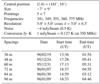
Table 1. Observational details of the Auriga field.
Central position (l,b)=(161◦,16◦)
Size ∼7◦×9◦
Pointings 5×7
Frequencies 341, 349, 355, 360, 375 MHz Resolution 5.00×5.00cosecδ=5.00×6.30 Noise ∼4 mJy/beam (0.5 K)
Conversion Jy–K 1 mJy/beam=0.127 K (at 350 MHz)
Spacings Date Start time End time
(UT) (UT)
36 m 96/02/19 13:36 01:54
48 m 95/12/24 17:28 05:41
60 m 95/12/31 17:13 05:31
72 m 96/01/07 16:37 04:55
84 m 96/01/30 14:59 03:12
96 m 96/01/09 16:33 04:46
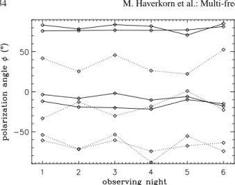
point sources (in the Q- and U-maps at∼10 resolution). The result is shown in Fig. 1 for 4 strong sources and 4 weaker sources. The strong sources have a signal-to-noiseσ=2−3.5 for an individual 12 hr observation, which corresponds to an uncertainty in polarization angleσφ≈10◦. The signal-to-noise
of the weaker sources isσ=1.2−1.5 (σφ≈22◦). From Fig. 1
we conclude that differential Faraday rotation between the six 12 hr observations is negligible to within the uncertainties with which it can be measured from the point sources.
We can estimate the RM contribution of the ionosphere from the earth magnetic field and the electron density in the ionosphere. The contribution of the ionospheric Faraday rota-tion is estimated as follows. The total electron content (TEC) in the ionosphere above Westerbork at night, in a solar mini-mum, and in winter is minimal: TEC≈2.2×10¹⁶electrons m−2 (Campbell, private communication). The Auriga field at decli-nationδ=52.5◦is almost in the zenith at Westerbork at hour angle zero. If we assume a vertical component of the earth magnetic field of 0.5 G towards us, and a path length through the ionosphere of 300 km, the RM caused by the ionosphere is 0.3 rad m−2 at hour angle zero. At larger hour angles, this is even less. So we expect the rotation measure values given in this paper not to be affected by ionospheric Faraday rotation by more than 0.5 rad m−2.
2.1. Missing large-scale structure
Fig. 1. Polarization angle variation over six 12 hr observations, for 8 extragalactic point sources. Four sources denoted by the solid lines are relatively strong (σ=2−3.5 for one 12 hr measurement), the dotted lines are sources withσ=1.2−1.5. Little angle variation over nights points to constant ionospheric Faraday rotation.
3. Total intensity and linear polarization maps
3.1. Total intensity
In the left-hand panel of Fig. 2 we show the map of total inten-sity I at 349 MHz with a resolution of 5.00×6.30. Point sources were removed down to the confusion limit of 5 mJy/beam.
I has a Gaussian distribution around zero with width σI = 1.3 K (while the noise, computed from V maps, is σV = 0.5 K), and is distributed around zero due to the insensitiv-ity of the interferometer to scales >∼1◦. From the continuum single-dish survey at 408 MHz (Haslam et al. 1981, 1982), the I-background at 408 MHz in this region of the sky is es-timated to be∼33 K with a temperature uncertainty of∼10% and including the 2.7 K contribution of the cosmic microwave background. Assuming a temperature spectral index of−2.7, the backgrounds at the lowest (341 MHz) and the highest (375 MHz) frequency of observation are ∼49 K and∼38 K, respectively. Of these, approximately 25% is due to sources, as estimated from source counts (Bridle et al. 1972), and assum-ing the spectral index of the Galactic background and the extra-galactic sources to be identical. We thus estimate the tempera-tures of the diffuse Galactic background at 341 and 375 MHz to be 37 and 29 K, respectively.
3.2. Polarized intensity
In the right-hand panel of Fig. 2 we show the map of polarized intensity at 349 MHz, with a resolution of 5.00×6.30. The noise in this map is∼0.5 K, and the polarized brightness temperature goes up to∼13 K, with an average value of∼2.3 K.
The map shows cloudy structure of a degree to a few de-grees in extent, with linear features that are sometimes paral-lel to the Galactic plane. In addition, a pattern of black nar-row wiggly canals is visible (see e.g. the canal around (α,δ)= (92.7◦, 49◦−51◦)). These canals are all one synthesized beam wide and are most likely due to beam depolarization. They separate regions of fairly constant polarization angle between
which the difference in polarization angle is approximately 90◦ (±n 180◦, n = 1,2,3. . .) (Haverkorn et al. 2000). A change of 90◦ (or 270◦, 450◦ etc.) in polarization angle within one
beam cancels the polarized intensity in the beam; therefore
these canals appear black in Fig. 2. Hence, the canals are not physical structures, but the reflection of specific features in the distribution of polarization angle. Such canals have also been detected by others at higher frequencies (e.g. Uyanıker et al. 1999; Gaensler et al. 2001). It must be appreciated that the canals represent an extreme case of beam depolarization. Beam depolarization is much more wide-spread if the polarization an-gle varies on the scale of the beam or on smaller scales, but in general its effect is (much) less than in the canals. Therefore, with the exception of the canals, beam depolarization does not leave easily visible traces in the polarized intensity distribution. An alternative explanation for depolarized regions accom-panied by a change in polarization angle of 90◦ is so-called depth depolarization or differential Faraday rotation. If the magnetic field in the medium is uniform, depolarization along the line of sight causes depolarized regions at certain RM val-ues (Sokoloff et al. 1998). However, in this scenario, it is hard to explain why the canals are all exactly one beam wide. Furthermore, the canals should shift in position with frequency, which is not observed. For an extended discussion on the possi-ble causes of polarization canals, see Haverkorn et al. (2003b). There is no obvious structure in Stokes I, and if there is any, it does not appear to be correlated with the structure in P. This is not typical for the Auriga field, but it is true in all fields observed so far with the WSRT at∼350 MHz (Katgert & de Bruyn 1999; Haverkorn et al. 2003a; Schnitzeler et al. in prep.). We have estimated the amount of correlation between to-tal and polarized intensity by deriving the correlation coeffi -cient C, where C( f, g) of the observables f (x, y) andg(x, y) is defined as
C( f, g)=
P
i,j
fi j−f gi j−g
qP
i,j
fi j−f
2 P
i,j
gi j−g
2 (1)
where f is the average value of f (x, y), fi j= f (xi, yj), summa-tion is over i=1,Nxand j=1,Ny, and Nxand Nyis the
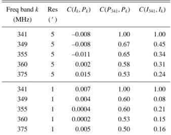
num-ber of data points in the x- andy-directions, respectively. The correlation coefficients between P and I, and between P and be-tween I at different frequencies are given in Table 2. Both the observed correlation coefficients at the maximum resolution of about 10, as well as those of the 50resolution data are given.
Fig. 2. Map of the total intensity I (left) and polarized intensity P (right) at 349 MHz, on the same brightness scale. The maps are smoothed to a resolution of 5.00×6.30. White denotes high intensity, up to a maximum of∼13 K. Superimposed in the right map are lines of constant Galactic latitude, at latitudes of 13◦, 16◦and 19◦.
Table 2. Correlation coefficients for correlations between P and I, be-tween I in different frequency bands and between P in different fre-quency bands, for tapered data and full resolution data.
Freq band k Res C(Ik,Pk) C(P341,Pk) C(I341,Ik) (MHz) (0)
341 5 –0.008 1.00 1.00
349 5 –0.008 0.67 0.45
355 5 –0.011 0.65 0.34
360 5 0.002 0.58 0.31
375 5 0.015 0.53 0.24
341 1 0.007 1.00 1.00
349 1 0.004 0.60 0.08
355 1 0.0004 0.60 0.21
360 1 0.0002 0.53 0.15
375 1 0.005 0.50 0.16
3.3. Polarization angle
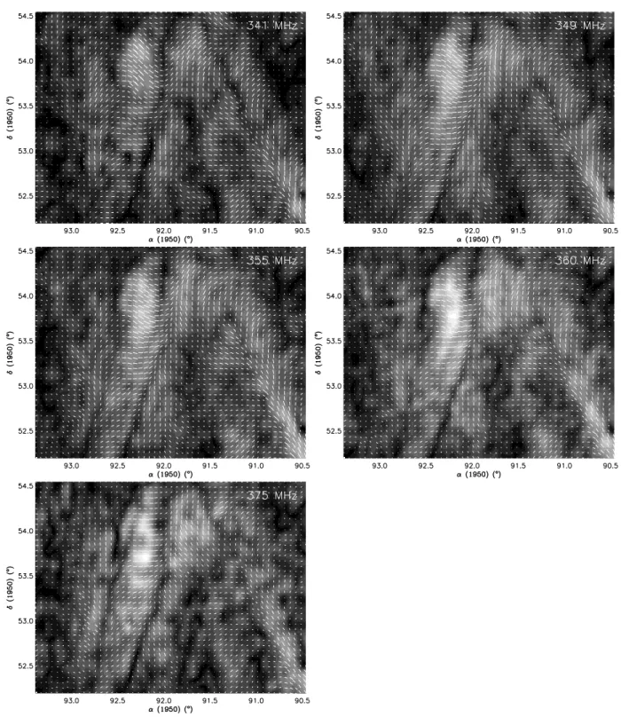
In Fig. 3 we show, for a 3◦×2◦subfield slightly northwest of the center of the mosaic, maps of polarized intensity P (grey scale) and polarization angleφ(superimposed pseudo-vectors) in the 5 frequency bands. In the grey scale, which has 5 samples per
linear beam width, white corresponds to high P. The length of the vectors (one per beam) scales with polarized intensity. The amount of structure in polarization angle is highly variable. At high polarized intensities, the polarization angles mostly vary quite smoothly. However, there are also abrupt changes on the scale of a beam, the most conspicuous of which give rise to the depolarization canals.
4. Faraday rotation
4.1. The derivation of rotation measures
The rotation measure (RM) of the Faraday-rotating material follows from φ(λ2) ∝ RMλ2. As φ = 0.5 arctan(U/Q),2 the values of polarization angle are ambiguous over±n 180◦
(n = 1,2,3, . . .) because a value of angle(Q,U) is
ambigu-ous over±n 360◦. For most beams, it was possible to obtain a linear φ(λ2)-relation by using angles with a minimum an-gle difference between neighboring frequency bands. Only in about 1% of the data, addition or subtraction 180◦to the polar-ization angle in at least one of the frequency bands was needed. One could increase RMs by adding or subtracting multiples of 180◦, but that would lead to RMs in excess of 100 rad m−2. If such high RMs were real, bandwidth depolarization (see Sect. 5) would have totally annulled any polarized signal.
Fig. 3. Five maps of a part of the Auriga region at frequencies 341, 349, 355, 360 and 375 MHz. The grey scale is polarized intensity P, oversampled 5 times, where white is high intensity. Maximum P (in the 375 MHz band) is approximately 13 K. Superimposed are polarization pseudo-vectors, where each line denotes an independent synthesized beam.
In addition, the RMs we obtain using the criterion of min-imum angle differences (of order of 10 rad m−2) were also obtained in other observations in this direction (Bingham & Shakeshaft 1967; Spoelstra 1984). So we conclude there are hardly any 180◦-ambiguities in polarization angle and we use the minimum angle difference between frequency bands to de-termine RMs.
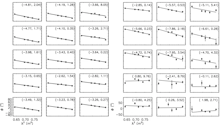
Fig. 4. Two typical parts of 3×5 beams in the observed field, represented in small graphs of polarization angleφagainstλ2, one graph per independent synthesized beam. The left 3×5 graphs are taken from a part of the field with high polarized intensity (σ >∼15 per frequency band), the right part from a region of lower intensity (σ≈5). The values within parentheses above each graph are RM and reducedχ2, respectively. In general, RMs are more regular and alike over several beams in high polarized intensity regions, but there is coherence in RM in lower P regions as well.
high P regions than in lower P regions, but in the larger part of the Auriga field RMs are very well-determined.
4.2. The distribution of rotation measures
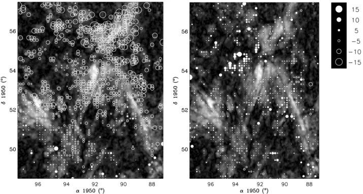
The RMs in the Auriga-field are plotted as circles in Fig. 5. Filled circles denote positive values, open circles negative, and the diameters of the circles are proportional to RM. For clarity, we only show the RMs for one in four independent beams. In addition, RMs are only shown when they were reliably deter-mined, i.e. for the average polarized intensityhPi > 5σ, and for reducedχ2of the fit<2.
The left panel shows RM as determined from the obser-vations. Most RMs are negative; the few positive values oc-cur for δ <∼ 52◦, while the largest negative values occur for
δ >∼55◦. We modeled this systematic variation by a large-scale linear gradient, and find a gradient of about 1 rad m−2per de-gree, with the steepest slope along position angle (from north through east) of−20◦.
The average RM, i.e. the RM value in the center of the fitted
RM-plane, over the field is RM0 ≈ −3.4 rad m−2. Subtracting the best-fit gradient from the RM distribution yields the RMs shown in the right-hand panel in Fig. 5 with only small-sale structure in RM. The distribution of small-scale RMs (i.e. RM where the large-scale gradient is subtracted) is significantly narrower than the total RM distribution (σRM =1.4 K instead
of 2.3 K), and is more symmetrical, as is shown in Fig. 6, where the two histograms are compared.
The decomposition of the RM-distribution into a constant component, a gradient, and a small-scale component is not physical, as there is probably structure on all scales. However, for our purpose it is a good approximation, and it allows us to estimate the large-scale and random components of the Galactic magnetic field, see Sect. 7.
4.3. Structure in RM on arcminute scales
Fig. 5. Rotation measures given as circles with a diameter proportional to the magnitude of the RM, superimposed over P at 349 MHz in grey scale. The scaling is in rad m−2. RMs are only shown if P>5σand reducedχ2 <2, and in both directions, only every second independent beam is plotted for clarity. The right map shows the same data where the best-fitting linear gradient in RM is subtracted.
Fig. 6. Histogram of RMs in the Auriga field. The dashed line gives the distribution of all “reliably determined” RMs, i.e. where P>5σand reducedχ2 <2. The solid line gives the reliably determined RM dis-tribution after subtracting a best-fit linear RM gradient from the data. Dotted lines show Gaussian fits to the two histograms.
that produces Faraday rotation and that emits synchrotron radi-ation show that the RM can change sign without a correspond-ing change in the direction of the magnetic field (Sokoloffet al. 1998; Chi et al. 1997).
5. The structure in
P, and the implied properties
of the ISM
As I and P are uncorrelated, the structure in P cannot be caused by structure in emission, but instead is created by several in-strumental and/or depolarization effects. We discuss these pro-cesses in detail in two forthcoming papers for several fields of
Fig. 7. White symbols and lines are plots ofφ againstλ2 and their linear fits, one for each independent beam, so that the slope is RM. Sudden RM changes occur over one beam width. The grey scale is polarized intensity at 349 MHz oversampled by a factor of 5. Maximum P (lightest grey) is∼40 mJy/beam, while in the bottom left pixel P is set to zero for comparison.
observation, among which the Auriga field (Haverkorn et al. 2003b,c). Here we summarize them, and discuss the results for the Auriga region.
Faraday-rotated by the screen have averages very close to zero (even if the background was uniformly polarized). As a result, the missing short-spacing information does not produce offsets. For our frequencies the latter is true ifσRM >∼1.8 rad m−2. In the Auriga region, this condition is met in essentially all of the subfields of the mosaic. Furthermore, a test in which offsets are added (described in the papers referred to above) to produce better linearity of theφ(λ2)-relation, did not result in reliable non-zero offsets.
Structure in P could also be generated by non-constant, but high, RM values as a result of bandwidth depolarization. Summation of polarization vectors with different angles in a frequency band will reduce the polarized intensity. The amount of depolarization depends on the spread in polarization angle within the band which, in turn, depends on the RM and the width of the frequency band. For the RMs of order 10 rad m−2 and our bandwidth of 5 MHz the effect is negligible.
A special kind of structure in P is due to beam depolar-ization, viz. the cancellation of polarization by vector sum-mation across the beam defined by the instrument. This is a 2-dimensional summation of polarization vectors across the plane of the sky, which is probably responsible for the depolar-ization canals. It certainly cannot produce all of the structure in P because it occurs on a single, small scale, whereas P has structure on a large range of scales.
Finally, depth depolarization occurs along the line of sight in a medium that both emits synchrotron radiation and pro-duces Faraday rotation. It must be responsible for a large part of the structure in P. The ISM in the Galactic disk most likely is such a medium. The Galactic synchrotron emission has been modeled by Beuermann et al. (1985) as the sum of two contri-butions: the thin disk with a half equivalent width of∼180 pc, which coincides with the stellar disk, and a thick disk of half equivalent width ∼1800 pc (where the galactocentric radius of the sun is assumed R = 10 kpc). Thermal electrons exist also out to a scale height of approximately a kpc, contained in the Reynolds layer (Reynolds 1989, 1991). So up to a height of about a kpc, the medium probably consists of both emit-ting and Faraday-rotaemit-ting material. In such a medium, the po-larization plane of the radiation emitted at different depths is Faraday-rotated by different amounts along the line of sight. Therefore the polarization vectors cancel partly, causing depo-larization along the line of sight even if the magnetic field and thermal and relativistic electron densities are constant (diff er-ential Faraday rotation, see Gardner & Whiteoak 1966; Burn 1966; Sokoloffet al. 1998). If the medium contains a random magnetic field, the polarization plane of the synchrotron emis-sion will vary along the line of sight causing extra depolariza-tion in addidepolariza-tion to the differential Faraday rotation (called in-ternal Faraday dispersion). We will refer to the combination of the two mechanisms along one line of sight as depth depolar-ization, thus adopting the terminology proposed by Landecker et al. (2001).
Depth depolarization is the dominant depolarization pro-cess in the Auriga field. We constructed a numerical model in Haverkorn et al. (2003c) to evaluate if depth depolarization can indeed be held responsible for most of the structure in P, in the Auriga region as well as in the other region that we studied. At
the same time, the model makes it possible to estimate the con-ditions in the warm component of the ISM. The model consists of a layer corresponding to the thin Galactic disk, where ran-dom magnetic fields on small scales are present, and a constant background polarized radiation.
In the model, the thin disk (with height h) is divided in cells of a single size d, which contain a random magnetic field com-ponent Bran and a regular magnetic field Breg. The amplitude of Bran is constant, but in each cell its direction is randomly chosen. Each cell emits synchrotron radiation, proportional to
B2
⊥ = (Bran,⊥)2+(Breg,⊥)2, where we add energy densities
be-cause the two components are physically separated different fields. Only a fraction f of the cells contains thermal electrons, and therefore Faraday-rotates all incoming radiation (to repre-sent the filling factor f of the warm ISM).
We distinguish several kinds of model parameters. First, we have input parameters with values taken from the literature; these are thermal electron density ne=0.08 cm−3, filling factor
f =0.2 (both from Reynolds 1991), and height of the Galactic thin disk h=180 pc (Beuermann et al. 1985). Secondly, there are constraints from the observations of the Auriga field, viz. the width, shape and mean of the Q, U, I and RM distribu-tions. In addition, we define parameters without observational constraints, such as cell size d and emissivity per cell, which we vary in a attempt to constrain them from the model given the observational constraints. Finally, there are parameters that can be adjusted and optimized for each allowed cell size and emissivity per cell, like the random and regular magnetic field components and background intensity.
Using the observations of the Auriga region to constrain the parameters in the depth depolarization model, we obtain the following estimates. The cell size d is probably in the range from 5–20 pc, the random component of the magnetic field Branis about 1µG for a cell size of 5 pc or larger, and up to 4µG for smaller cell sizes. With the estimate of the large-scale, regular field (∼3µG) this leads to a value of about 0.3 to 1.3 for Bran/Breg. This is lower than most other estimates of Bran/Breg in the literature, which seem to indicate a value larger than 1. One possible explanation for this discrepancy is the fact that the Auriga region is not very large. Therefore ran-dom magnetic field components that project to angular scales larger than a few degrees will have been interpreted as ponents of the regular field. If such large-scale random com-ponents exist, this effect will artificially decrease Bran/Breg. Secondly, the Auriga field was selected for its conspicuous polarization structure, and high polarized intensity in general indicates a more regular magnetic field structure. Finally, the Auriga region is observed in an inter-arm region. The next spi-ral arm, the Perseus arm, is more than 2 kpc away, and we expect that at these frequencies, all polarized emission from the Perseus arm is depolarized. There are indications that in the inter-arm region, the regular magnetic field component is higher than the random magnetic field component (Han & Qiao 1994; Indrani & Deshpande 1998; Beck 2001).
Fig. 8. The amount of polarization contributed by a certain cell, against the distance to that cell, in a single-cell-size model of polarized radiation propagating through a magneto-ionized medium.
Table 3. Extragalactic sources in the Auriga region. The second col-umn gives position, and the third RMs. Reducedχ2of theφ(λ2) rela-tion is given in Col. 4. Columns 5–7 give resp. P, I (both in mJy/beam) and percentage of polarization p averaged over the five frequency bands.
No. (α, δ) (◦, ◦) RM (rad m−2) χ2 hPi hIi hpi
1 [ 97.9, 55.3 ] 7.4±0.2 12.9 45.6 2021 2.3 2 [ 97.7, 53.6 ] 12.9±0.3 3.1 14.9 216 6.9 3 [ 96.6, 53.3 ] 6.6±0.4 1.7 15.0 224 6.7 4 [ 96.5, 54.1 ] 5.7±0.4 3.7 11.9 380 3.1 5 [ 95.3, 50.8 ] 0.6±0.4 1.6 14.7 165 8.8 6 [ 95.2, 50.8 ] 3.1±0.4 0.2 14.7 197 7.5 7 [ 94.7, 54.8 ] 7.9±0.3 3.0 18.8 282 6.7 8 [ 93.4, 55.6 ] 6.3±0.2 1.1 21.3 180 11.8 9 [ 92.3, 52.9 ] 2.7±0.1 6.1 35.8 1222 2.9 10 [ 90.3, 50.4 ] −10.2±1.4 4.4 7.4 168 4.4 11 [ 89.3, 55.0 ] 3.0±0.4 1.4 11.6 340 3.4 12 [ 89.2, 52.5 ] −8.1±0.1 12.7 22.1 477 4.6 13 [ 89.0, 52.3 ] −13.6±0.4 5.8 14 237 5.9
indications that structure exists in the ISM on many scales (Armstrong et al. 1995; Minter & Spangler 1996).
The distance out to which polarized radiation is not de-polarized by depth depolarization, as derived from the model, is shown in Fig. 8. The total path length through the medium containing small-scale structure was about 600 pc, which cor-responds to a height of the thin disk of about 150 pc for the Auriga latitude of∼16◦. Radiation emitted at large distances is depolarized more than emission from nearby, but there is no definite polarization horizon due to depth depolarization. Beam depolarization can cause a polarization horizon, as structure further away will be on smaller angular scales, which causes more beam depolarization (Landecker et al. 2001).
6. Polarized extragalactic point sources
Thirteen polarized extragalactic point sources in the Auriga-field were selected based on three selection criteria: (1) signal-to-noiseσ >3 in P at all frequencies, (2) the degree of polar-ization p is higher than 1% at all frequencies (because a lower polarization degree can also be caused by instrumental polar-ization, see Sect. 2), and (3) the source does not lie too far at
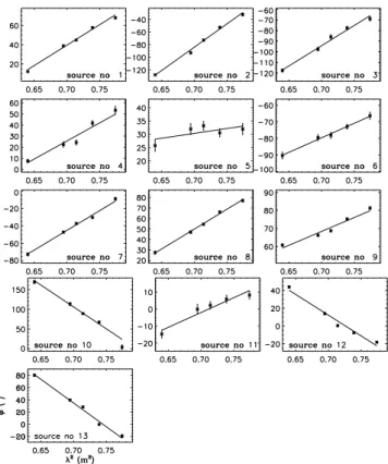
Fig. 9. Plots of polarization angleφ againstλ2 for the 13 polarized extragalactic sources in Table 3. Note that the scaling of theφ-axis differs for each source.
the edge of the field away from any pointing center, to limit the contribution from instrumental polarization. The 13 sources are all detected in the 10resolution data, and most of them are unresolved at that resolution. Their RMs vary from approxi-mately−13 to 13 rad m−2.
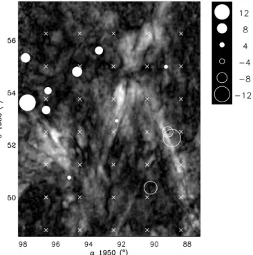
The relevant properties of the sources are given in Table 3, where the second column gives the right ascension and declina-tion, Col. 3 the RM, and Col. 4 the reducedχ2of theφ(λ2)-fits. Columns 5, 6, and 7 give the values of P, I and percentage of polarization p respectively, averaged over all frequency bands. Figure 9 shows the polarization angleφplotted againstλ2 for each point source. In Fig. 10, we show the 13 sources overlaid on a grey scale plot of polarized intensity at 349 MHz, with their RMs indicated. The diameter of the symbol and its shad-ing indicate the value of RM.
Sources 1 and 2 could have a significant contribution of in-strumental polarization, because they are observed in only one pointing center and are located about 0.8◦to 1◦away from the pointing center. Nevertheless, they show linearφ(λ2)-relations, which indicates that instrumental polarization is not important. These sources are therefore included in the analysis.
Fig. 10. RMs of the 13 polarized extragalactic point sources in the Auriga field in circles, overlaid on P at 349 MHz. Filled circles are positive RMs, open circles negative. The crosses denote the pointing centers, and the scaling is in rad m−2.
“internal” RM contribution from the extragalactic source or a halo around it of∼5 rad m−2.
The change of sign of RM of the extragalactic sources within the observed region indicates a reversal in the Galactic magnetic field. (Unlike the diffuse emission, sign changes in RMs of extragalactic sources cannot be due to depolariza-tion effects.) The reversal exists on scales larger than our field of view, as is shown in Fig. 11, where we combine the RMs of our sources with those from the literature. The circles are our sources, the squares indicate sources that were detected by Simard-Normandin et al. (1981) and/or by Tabara & Inoue (1980), and the one triangle indicates the only pulsar nearby (Hamilton & Lyne 1987). The numbers next to the squares and triangle give the magnitude of RM of the source (the diam-eter of the symbol is only proportional to RM up to RM = 15 rad m−2). One source at (α, δ) = (91.25◦,48◦) was omit-ted, because Simard-Normandin et al. give RM= 34 rad m−2 and Tabara & Inoue give RM = −64.9 rad m−2. The source distribution shows a clear magnetic field reversal, which is not on Galactic scale but on smaller scales, as is shown in Figs. 1 and 2 of Simard-Normandin & Kronberg (1980), which show
RMs of extragalactic sources over the whole sky.
The gradient in RM measured in the extragalactic point sources is completely unrelated and almost perpendicular to the structure in RM from the diffuse emission. This can be ex-plained from the widely different path lengths that extragalac-tic sources and diffuse emission probe. Diffuse emission can only be observed out to a distance of a few hundred pc to a kpc, as radiation from further away will be mostly depolar-ized. On the contrary, extragalactic sources are Faraday-rotated over the complete path length through the Milky Way of many
Fig. 11. RMs of extragalactic point sources and of one pulsar. The circles are the point sources detected in the Auriga field, where the radius of the circle is proportional to the magnitude of RM. Squares are extragalactic point sources detected by Simard-Normandin et al. (1981) and/or by Tabara & Inoue (1980), and the one triangle in the field denotes the only pulsar near the Auriga field (Hamilton & Lyne 1987). Values of the RM are written next to the sources, and for RM< 15 rad m−2the radius of the symbol is proportional to RM.
kiloparsecs long. Therefore, the RM structure from diffuse ra-diation and from extragalactic sources gives information about different regions in the Galaxy.
7. Discussion
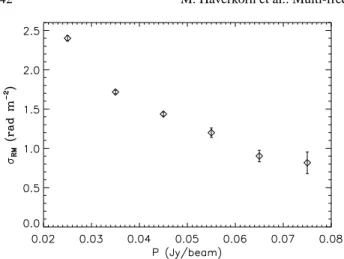
7.1. High P-structures and alignment with the Galactic plane
Fig. 12. Width of a Gaussian fit to the RM distributionσRMfor a range of P, where P is divided in bins of 0.01 Jy/beam.
effect cannot be due to noise. For the two intervals of high-est P (0.08–0.09 Jy/beam and 0.09–0.10 Jy/beam), not shown in Fig. 12, no Gaussian fit could be made, as the distributions were bimodal. The peaks in these bimodal distributions corre-spond to two spatially coherent structures, which are shown in the two panels of Fig. 13. In the region around (α, δ) = (94.6◦,51.8◦),−1.5 <∼ RM <∼ 0 rad m−2, while in the region around (α, δ)=(92.2◦,53.8◦), 0<∼RM<∼1.3 rad m−2. Clearly,
RM is indeed very uniform in regions of high polarization. The
low variation in RM is also reflected in the uniformity of the polarization angles.
A constant RM over a certain area sets an upper limit on structure in magnetic field and thermal electron density. The fact that some of the filamentary structure in P is aligned with Galactic latitude suggests a magnetic origin, although stratifi-cation of neover Galactic latitude can contribute as well. For variation of polarization angle over the filament of less than about 20◦ (from Fig. 13), ∆RM <∼ 0.5 rad m−2 is needed. If magnetic field structure would be the same over the entire path length towards the filament, and assuming ne = 0.08 cm−3, this requires a magnetic field change ∆Bk <∼ 0.01 µG with a polarization depth of 600 pc. Even if the filamentary struc-tures are sheet-like with a constant magnetic field over a large part of the path length, or if the polarization horizon is lo-cally much shorter than the highly uncertain value of 600 pc, the upper limit to∆B is very low. Therefore, this structure of
high P aligned with Galactic latitude indicates the existence of long filaments or sheets parallel to the Galactic plane of highly uniform magnetic field and thermal electron density. As back-and/or foreground structure can also imprint structure in RM, these regions may well be characterized by low thermal elec-tron density.
7.2. The Galactic magnetic field
The Auriga field of 7◦×9◦represents only 0.1% of the sky, and is therefore by itself not very well suited for an analysis of the global properties of the Galactic magnetic field. However, we can estimate strength and direction of the regular component of
Fig. 13. Two areas in the P map at 349 MHz with highest P (>80 mJy/beam). Overlaid pseudo-vectors are polarization angles, showing a minimal change in angle for high P.
the Galactic magnetic field from the distribution of RMs of the diffuse radiation and of the extragalactic sources over the field. First, we need to determine how much of the RM gra-dient seen in the diffuse emission is caused by ne, and how much by Bk. Independent measurements of ne can be ob-tained from the emission measure E M = R n2
e dl, as mea-sured with the Wisconsin HαMapper survey (WHAM, Haffner et al., in prep., Reynolds et al. 1998), shown in Fig. 14. As the resolution is about a degree, the WHAM survey cannot be used to determine small-scale structure in ne, but gives an estimate of the global gradient in ne over the field. From north to south, the Hα observations show an increase from about 1 to 5 Rayleighs (1 Rayleigh is equal to a brightness of 106/4πphotons cm−2s−1ster−1, and corresponds to an E M of about 2 cm−6pc for gas with a temperature T =10 000 K). The small enhancement in E M at (α, δ) = (94.8◦,55.5◦) is probably related to the ancient planetary nebula PuWe1 (PW1, Tweedy & Kwitter 1996). Note that the Hα emission probes a longer line of sight than the diffuse polarization, and is ve-locity integrated over−80 to 80 km s−1LSR, so complete cor-respondence is not expected. However, a gradient in RM that was solely due to the ne-gradient would have a sign opposite to that of the observed RM-gradient. Therefore, the observed gradient in RM must be due to a gradient in the parallel com-ponent of the magnetic field. If the gradient in Hαoriginates in the same medium as the polarized radiation, the gradient in magnetic field must even be large enough to compensate the gradient in electron density in the opposite direction.
Fig. 14. Superimposed circles are emission measures from the WHAM Hαsurvey, to a maximum intensity of∼5 Rayleigh, at a res-olution of one degree. The grey scale denotes P at 349 MHz.
the value of the RM gradient give two independent estimates of the regular magnetic field, if a certain pitch angle is as-sumed. Assuming a path length of 600 pc and electron den-sity ne = 0.08 cm−3, the two magnetic field determinations agree on a regular magnetic field of Breg ≈ 1 µG for a pitch angle p = −14◦, in agreement with earlier estimates (Vall´ee 1995).
The gradient in the RMs of the extragalactic sources does not show a longitudinal component at all, contrary to that in the RMs of the diffuse polarization observations. This indicates that other large-scale magnetic fields become important, fields that vary on scales larger than our field. Observations of halos of external galaxies (e.g., Dumke et al. 1995) have shown that cell sizes in the Galactic halo are much larger than in the disk, from 100–1000 pc. Even at a distance of 3000 pc, the size of the total Auriga field is∼400 pc, so big cells in the halo could be responsible for a considerable part of what we call the regular component of the magnetic field, as measured in the RMs of the extragalactic sources.
We subtracted the gradient of the diffuse emission from the gradient in the RMs of the extragalactic sources, after which a gradient in RM of∆RM ≈ 3.6 rad m−2 in position angle 54◦ remains (only deviating by about 10◦ from the direction per-pendicular to the Galactic plane). This indicates a regular mag-netic field of about 1 µG in this direction, assuming that ne and B remain constant over a total line of sight of 3000 pc. The magnetic field strengths actually present in the medium will be higher if the field varies along the line of sight.
8. Conclusions
Multi-frequency polarization observations of the diffuse Galactic background yield information on structure in the Galactic warm gas and magnetic field.
The multi-frequency WSRT observations of a region of size ∼7◦ × 9◦ at l = 161◦, b = 16◦ in the constellation Auriga show a smooth total intensity I, but abundant struc-ture in Stokes parameters Q and U on several scales, with a maximum Tb,pol≈13 K (about 30% polarization). Filamentary structure up to many degrees long is present in P, sometimes aligned with Galactic latitude. In addition, narrow, one-beam wide depolarization canals are most likely created by beam de-polarization and may well indicate abrupt RM changes. As the polarization structure is uncorrelated to I, the structure in P cannot be created by variations in synchrotron emission, but has to be due to Faraday rotation and depolarization mecha-nisms.
Rotation measure maps show abundant structure on many scales, including a linear gradient of∼1 rad m−2 per degree in the direction of positive Galactic longitude and an average
RM0 ≈ −3.4 rad m−2. The gradient is consistent with the reg-ular Galactic magnetic field if its strength is Breg ≈1µG and the field is azimuthally oriented with a pitch angle p ≈ −14◦. Ubiquitous structure is present in the RM map on beam size scales (50), indicating significant changes in magnetic field and/or thermal electron density over very small spatial scales.
There are two dominant depolarization mechanisms which create structure in P in the Auriga field. First, beam depolariza-tion (i.e. depolarizadepolariza-tion due to averaging out polarizadepolariza-tion angle structure within one beam width) most likely creates the canals, and is important in regions of low P. Additional depolarization is needed to explain the observed P distribution, which is only possible if the medium both Faraday-rotates and emits syn-chrotron emission. Then, emission originating in the medium can be depolarized along its path towards the observer, so-called depth depolarization. The polarization angle along the path can vary due to Faraday rotation, or due to varying intrin-sic polarization angle of the emission. This indicates a varying magnetic field, which however is constrained by the upper limit on structure in I. A depth depolarization model was constructed of a layer of cells with varying magnetic fields and a constant background polarization. Constraints from the Auriga observa-tions give estimates for several parameters in the ISM. The cell size of structure in the ISM is constrained to∼15 pc, and the ratio of random to regular field is 0.7±0.5.
Thirteen extragalactic sources in the Auriga field also show a gradient in RM, but roughly in the direction of Galactic lati-tude, which is perpendicular to the gradient in the diffuse emis-sion. The RM distributions from diffuse radiation and from extragalactic point sources are so different because the dif-fuse radiation mostly probes the first few hundred parsecs, whereas RMs from the point sources are built up along the en-tire line of sight through the Milky Way. RMs of extragalactic sources change sign over the field, which indicates a local re-versal of the magnetic field.
Acknowledgements. We thank R. Beck, E. Berkhuijsen and F. Heitsch
Radio Telescope is operated by the Netherlands Foundation for Research in Astronomy (ASTRON) with financial support from the Netherlands Organization for Scientific Research (NWO). The Wisconsin H-Alpha Mapper is funded by the National Science Foundation. MH is supported by NWO grant 614-21-006.
References
Armstrong, J. W., Rickett, B. J., & Spangler, S. R. 1995, ApJ 443, 209 Baars, J. W. M., Genzel, R., Pauliny-Toth, I. I. K., & Witzel, A. 1977,
A&A, 61, 99
Beck, R. 2001, SSRv, 99, 243
Beck, R., Brandenburg, A., Moss, D., Shukurov, A., & Sokoloff, D. 1996, ARA&A, 34, 155
Beuermann, K., Kanbach, G., & Berkhuijsen, E. M. 1985, A&A, 153, 17
Bingham, R. G., & Shakeshaft, J. R. 1967, MNRAS, 136, 347 Bridle, A. H., Davis, M. M., Fomalont, E. B., & Lequeux, J. 1972,
NPhS, 235, 123
Brouw, W. N., & Spoelstra, T. A. T. 1976, A&AS, 26, 129 Brown, J. C., & Taylor, A. R. 2001, ApJ, 563, L31 Burn, B. J. 1966, MNRAS, 133, 67
Chi, X., Young, E. C. M., & Beck, R. 1997, A&A, 321, 71
Clegg, A. W., Cordes, J. M., Simonetti, J. H., & Kulkarni, S. R. 1992, ApJ, 386, 143
Dumke, M., Krause, M., Wielebinski, R., & Klein, U. 1995, A&A, 302, 691
Duncan, A. R., Reich, P., Reich, W., & F¨urst, E. 1999, A&A, 350, 447 Duncan, A. R., Haynes, R. F., Jones, K. L., & Stewart, R. T. 1997,
MNRAS, 291, 279
Ferri`ere, K. M. 2001, RvMP, 73, 1031
Gaensler, B. M., Dickey, J. M., McClure-Griffiths, N. M., et al. 2001, ApJ, 549, 959
Gardner, F. F., & Whiteoak, J. B. 1966, ARA&A, 4, 245
Haffner, L. M., Reynolds, R. J., & Tufte, S. L., et al., in preparation Han, J. L. 2001, in Astrophysical Polarized backgrounds, ed. by S.
Cecchini, S. Cortiglioni, R. Sault, & C. Sbarra
Han, J. L., Manchester, R. N., Berkhuijsen, E. M., & Beck, R. 1997, A&A, 322, 98
Han, J. L., Manchester, R. N., & Qiao, G. J. 1999, MNRAS, 306, 317 Han, J. L., & Qiao, G. J. 1994, A&A, 288, 759
Hamilton, P. A., & Lyne, A. G. 1987, MNRAS, 224, 1073
Haslam, C. G. T., Stoffel, H., Salter, C. J., & Wilson, W. E. 1982, A&AS, 47, 1
Haslam, C. G. T., Klein, U., Salter, C. J., Stoffel, H., et al. 1981, A&A, 100, 209
Haverkorn, M. 2002, Ph.D. Thesis, Leiden Observatory
Haverkorn, M., Katgert, P., & de Bruyn, A. G. 2003a, A&A, in press [astro-ph/0304087]
Haverkorn, M., Katgert, P., & de Bruyn, A. G. 2003b, A&A, submitted Haverkorn, M., Katgert, P., & de Bruyn, A. G. 2003c, A&A, submitted Haverkorn, M., Katgert, P., & de Bruyn, A. G. 2000, A&A, 356, L13 Heitsch, F., Mac Low, M.-M., & Klessen, R. 2001, ApJ, 547, 280 Indrani, C., & Deshpande, A. A. 1998, New Astron., 4, 331 Jones, T. J., Klebe, D., & Dickey, J. M. 1992, ApJ, 389, 602 Junkes, N., F¨urst, E., & Reich, W. 1987, A&AS, 69, 451
Katgert, P., & de Bruyn, A. G. 1999, in New perspectives on the in-terstellar medium, ed. A. R. Taylor, T. L. Landecker, & G. Joncas, 411
Landecker, T. L., Uyanıker, B., & Kothes, R. 2001, AAS, 199, #58.07 Leahy, J. P. 1987, MNRAS, 226, 433
Lyne, A. G., & Smith, F. G. 1989, MNRAS, 237, 533 Minter, A. H., & Balser, D. 1997, ApJ, 484, L133 Minter, A. H., & Spangler, S. R. 1996, ApJ, 458, 194 Ohno, H., & Shibata, S. 1993, MNRAS, 262, 953 Rand, R. J., & Kulkarni, S. R. 1989, ApJ, 343, 760 Rand, R. J., & Lyne, A. G. 1994, MNRAS, 68, 497
Rengelink, R. B., Tang, Y., de Bruyn, A. G., et al. 1997, A&AS, 124, 259
Reynolds, R. J. 1989, ApJ, 339, L29 Reynolds, R. J. 1991, ApJ, 372, L17
Reynolds, R. J., Tufte, S. L., Haffner, L. M., Jaehnig, K., & Percival, J. W. 1998, PASA, 15, 14
Shu, F. H. 1985, in The Milky Way Galaxy; Proc. of the 106th IAU Symp., 566
Simard-Normandin, M., & Kronberg, P. P. 1979, Nature, 279, 115 Simard-Normandin, M., & Kronberg, P. P. 1980, ApJ, 242, 74 Simard-Normandin, M., Kronberg, P. P., & Button, S. 1981, ApJS, 45,
97
Sofue, Y., & Fujimoto, M. 1983, ApJ, 265, 722
Sokoloff, D. D., Bykov, A. A., Shukurov, A., et al. 1998, MNRAS, 299, 189
Spoelstra, T. A. T. 1984, A&A, 135, 238 Tabara, H., & Inoue, M. 1980, A&AS, 39, 379 Tweedy, R. W., & Kwitter, K. B. 1996, ApJS, 107, 255
Uyanıker, B., F¨urst, E., Reich, W., Reich, P., & Wielebinski, R. 1999, A&AS, 138, 31
Vall´ee, J. P. 1983, A&A, 124, 147 Vall´ee, J. P. 1995, ApJ, 454, 119
V´azquez-Semadeni, E., Ostriker, E. C., Passot, T., Gammie, C. F., & Stone, J. M. 2000, in Protostars and Planets IV, ed. V. Mannings, A. P. Boss, & S. Russell, 3