VELOCITY-SPACE REASONING FOR INTERACTIVE SIMULATION OF DYNAMIC CROWD BEHAVIORS
Sujeong Kim
A dissertation submitted to the faculty of the University of North Carolina at Chapel Hill in partial fulfillment of the requirements for the degree of Doctor of Philosophy in the Department of
Computer Science.
Chapel Hill 2015
ABSTRACT
Sujeong Kim: Velocity-Space Reasoning for Interactive Simulation of Dynamic Crowd Behaviors (Under the direction of Dinesh Manocha and Ming C. Lin)
The problem of simulating a large number of independent entities, interacting with each other and moving through a shared space, has received considerable attention in computer graphics, biomechanics, psychology, robotics, architectural design, and pedestrian dynamics. One of the major challenges is to simulate the dynamic nature, variety, and subtle aspects of real-world crowd motions. Furthermore, many applications require the capabilities to simulate these movements and behaviors at interactive rates.
In this thesis, we present interactive methods for computing trajectory-level behaviors that capture various aspects of human crowds. At a microscopic level, we address the problem of modeling the local interactions. First, we simulate dynamic patterns of crowd behaviors using Attribution theory and General Adaptation Syndrome theory from psychology. Our model accounts for permanent, stable disposition and the dynamic nature of human behaviors that change in response to the situation. Second, we model physics-based interactions in dense crowds by combining velocity-based collision avoidance algorithms with external forces. Our approach is capable of modeling both physical forces and interactions between agents and obstacles, while also allowing the agents to anticipate and avoid upcoming collisions during local navigation.
ACKNOWLEDGEMENTS
I have been blessed to have the support of many people during my time at UNC. They have supported me during both the good and tough times and I would like to thank them for making this thesis a reality. First of all, I deeply thank my advisors, Dinesh Manocha and Ming C. Lin. They not only provided excellent vision and feedback about my goals and results, but also led me to extend my potential much further than what I thought would be possible.
I also cannot give enough thanks and credit to Stephen J. Guy who is my friend (thanks for the support during the tough times), collaborator (for the many papers we worked together) and committee member. I also am thankful for the support from the rest of my committee members: Carol O’Sullivan, who was also my mentor at Disney Research, helped me many times with great suggestions and feedback for my work. I appreciate Jan-Michael Frahm for introducing me to computer vision through his class which made me actually act on conducting a research in a new direction.
I cannot forget my friends and collaborators: Sean Curtis provided amazing tools and lots of advice both for research and school life. Aniket Bera, David Wilkie, and Wenxi Liu helped me a lot with my later work related to computer vision and robotics. To my other friends and GAMMA team members, too many to list here, I will never forget the great feedback and help in developing and polishing my work. I thank my friend Lenin Singaravelu, who patiently listened to all my complaints about anything and also helped proofreading the thesis.
TABLE OF CONTENTS
LIST OF TABLES . . . x
LIST OF FIGURES . . . xi
LIST OF ABBREVIATIONS . . . .xviii
1 Introduction . . . 1
1.1 Motivation . . . 1
1.2 Crowd Simulation . . . 2
1.2.1 Local Collision Avoidance in Velocity-Space Reasoning . . . 3
1.2.2 Modeling Local Interactions . . . 3
1.2.3 High-level Behavior Modeling . . . 5
1.2.4 Crowd Simulation for Robotics . . . 5
1.3 Thesis Statement . . . 6
1.4 Main Results . . . 7
1.4.1 Modeling Dynamic, Heterogeneous Behaviors . . . 8
1.4.2 Modeling Physical Interactions . . . 10
1.4.3 Adaptive Motion Model: Learning Individual Motion Parameters from Real World Crowd . . . 11
1.4.4 Time-varying Crowd Behavior Learning for Crowd Simulation . . . 12
2 Interactive Simulation of Dynamic Crowd Behaviors using General Adaptation Syndrome Theory. . . 15
2.1 Introduction. . . 15
2.2.2 Crowd Simulation . . . 18
2.2.2.1 Interactive Crowd Simulation . . . 18
2.2.2.2 Behavior Modeling . . . 18
2.3 Preliminaries and Overview . . . 19
2.3.1 Psychological Models of Stress. . . 20
2.3.2 General Adaptation Syndrome (GAS) . . . 20
2.3.3 Approximation of the GAS Model . . . 21
2.3.4 Overview of our Approach . . . 22
2.4 Modeling Stress and Stressors . . . 22
2.4.1 Perceived Stress . . . 23
2.4.2 Stressor Prototypes . . . 24
2.4.3 Stress Model . . . 25
2.5 Behavior Mapping . . . 26
2.5.1 Incorporation of Behavior Changes . . . 26
2.5.2 Coupling with Personality Attributes . . . 27
2.5.3 Modeling from Real-world Data . . . 28
2.6 Results . . . 28
2.6.1 Emergent Behaviors . . . 29
2.6.2 Validation . . . 30
2.6.3 Performance Results . . . 32
2.7 Conclusion . . . 33
3 Velocity-Based Modeling of Physical Interactions in Dense Crowds . . . 34
3.1 Introduction. . . 34
3.2 Related Work . . . 37
3.2.1 Multi-Agent Motion Models . . . 37
3.2.2 Dense Crowd Simulation . . . 37
3.2.4 Crowd Simulation in Game Engines . . . 39
3.3 Velocity-based Modeling of Physical Interactions . . . 39
3.3.1 Overview . . . 40
3.3.2 Anticipatory Collision Avoidance . . . 41
3.3.2.1 Agent-agent collision avoidance . . . 41
3.3.2.2 Agent-dynamic obstacle collision avoidance . . . 41
3.3.3 Constraints from Physical Forces . . . 42
3.3.3.1 Force computation . . . 42
3.3.3.2 Force constraints . . . 44
3.3.4 Benefits of Force Constraints . . . 45
3.4 Higher-Level Behavior Modeling . . . 46
3.4.1 The Behavior Finite State Machine . . . 46
3.5 Results . . . 48
3.5.1 Agent-Agent Interaction . . . 49
3.5.2 Agent-object Interaction . . . 50
3.5.3 Dodge-ball scenario . . . 52
3.5.4 Large-Scale Simulation: Tawaf Scenario . . . 54
3.5.4.1 Effect of physical interactions . . . 56
3.6 Analysis . . . 59
3.7 Conclusions and Future Work . . . 62
4 BRVO: Predicting Pedestrian Trajectories using Velocity-Space Reasoning . . . 64
4.1 Introduction. . . 64
4.2 Related Work . . . 66
4.2.1 Motion Models . . . 66
4.2.2 People-Tracking with Motion Models . . . 67
4.2.3 Robot Navigation in Crowds . . . 68
4.3.1 Motion Prediction Methods using Agent-Based Motion Models . . . 69
4.3.2 RVO Multi-Agent Simulation . . . 70
4.4 Bayesian-RVO . . . 72
4.4.1 Problem Definition . . . 72
4.4.2 Model Overview . . . 73
4.4.3 State Representation . . . 76
4.4.4 State Estimation . . . 76
4.4.5 Maximum Likelihood Estimation . . . 77
4.4.6 Implementation. . . 78
4.5 Results and Analysis . . . 80
4.5.1 Method Analysis . . . 82
4.5.1.1 EnKF for Online Learning . . . 82
4.5.1.2 Online vs Offline Learning . . . 82
4.5.1.3 EM based estimation refinement . . . 83
4.5.2 Environmental Variations . . . 85
4.5.2.1 Noisy Data . . . 85
4.5.2.2 Density Dependance . . . 87
4.5.2.3 Sampling Rate Variations . . . 90
4.5.3 Model Performance Comparison . . . 90
4.5.4 Analysis . . . 92
4.6 Robot Navigation with BRVO . . . 92
4.7 Conclusion and Future Work . . . 97
5 Interactive Data-Driven Crowd Simulation using Time Varying Pedestrian Dynamics. . . 98
5.1 Introduction. . . 98
5.2 Related Work . . . 100
5.2.1 Crowd Simulation . . . 101
5.2.3 Video Based Crowd Analysis . . . 102
5.3 Time Varying Pedestrian Dynamics . . . 103
5.3.1 Pedestrian State . . . 103
5.3.2 Pedestrian Dynamics . . . 104
5.3.3 State Estimation . . . 106
5.3.4 Dynamic Movement Flow Learning . . . 107
5.3.5 Entry-Points Learning . . . 109
5.4 Data-driven Crowd Simulation . . . 110
5.4.1 Pedestrian Dynamics Retrieval . . . 111
5.4.1.1 Adapting to Different Environments and Situations . . . 112
5.5 Results . . . 114
5.5.1 Scenarios . . . 115
5.6 Analysis and Comparisons . . . 119
5.6.1 Comparisons . . . 119
5.6.2 User Study . . . 120
5.7 Conclusions, Limitations and Future Work . . . 121
6 Conclusion and Future Work . . . 123
LIST OF TABLES
2.1 Data-driven stress parameters. Values derived from fitting our stress model
to street crossing data from Crompton [1979]. . . 32 2.2 Performance timings per frame. . . 32
3.1 Different interaction parameters for intentional behaviors and responsive behaviors . . 48 3.2 Performance on a single core for different scenarios. Our algorithm can
handle all of them at interactive rates. . . 60
4.1 Comparisons of different Bayesian learning algorithms Root mean squared error between the predicted position and ground truth position in
meters (best shown in bold). . . 82
5.1 Performance on a single core for different scenarios. We highlight the number of real and virtual pedestrians, the number of static obstacles, the number of frames of extracted trajectories and the time (in seconds) spent in different stages of our algorithm. Our learning and trajectory
computation algorithms can be used for interactive crowd simulations. . . 118 5.2 Comparison of similarity scores (higher is more similar). These
prelimi-nary results indicate that the use of our pedestrian dynamics learning algo-rithm to compute entry points and movement flows considerably improves the perceptual similarity of our simulation to the pedestrian movements in
LIST OF FIGURES
1.1 Components in Crowd Sim (colored outline) as related to techniques
(rounded rectangles) used in this thesis. . . 7 1.2 Opposing Group scenario. (a) Two opposing groups approach each other.
(b) Agents initially form natural lanes. (c) After experiencing stress from the alarm the lane formation breaks down into uncooperative, clogged and
congested behavior. . . 9 1.3 Average speed of agents in the Opposing Groups scenario at various
levels of stress. The Yerkes-Dodson Law states that stress should increase performance up to a point then decrease it, a result which is matched by
the proposed model. . . 10 1.4 Interactive Simulation of Physical Interactions between Agents,
Fur-niture in Office, and User-thrown Obstacles. Agents navigate to avoid office furniture (left). As users insert flying pink boxes into the scene, the
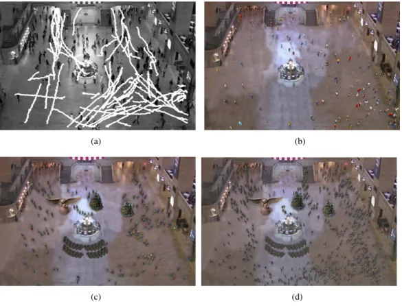
agents get pushed, collide into each other, and avoid falling objects (right). . . 11 1.5 Train Station scenario: (a) Original Video. We use the tracklet data
computed by the KLT algorithm as an input to our algorithm. We compute the pedestrian dynamics from the noise trajectories. (b) A frame from our data-driven crowd simulation algorithm in the same layout. (c) Crowd simulation in a modified layout as compared to the original video. (d) We increase the number of pedestrians in the scene. They have similar movement patterns as the original video and are combined with
density-dependent filters for plausible simulation. . . 14
2.1 Shibuya Crossing Scenario. A scenario simulating the scramble crossing near Shibuya metro station in Tokyo. (a) Agents start to walk quickly or jog when the walk signal begins flashing indicating little time left to cross. (b) When the light turns red, indicating no time left to cross safely, agents
experience a high level of stress and run aggressively to cross as quickly as possible. 15 2.2 General Adaptation Syndrome and approximation(a) GAS model of
the human response to stress. After an initial disturbance, the resistance level increases up to maximum capacity. If the stress is unresolved, the resistance gets weaker and is no longer effective (causes illness or death). (b) Our approximation of GAS model. We assume acute stress, i.e. no exhaustion stage. Instead, agents are relieved from stress when the stress is resolved. The shape of the response is determined by the stress
accumu-lation rateαand maximum capacityβ . . . 19 2.3 System OverviewDifferent levels of stressed behaviors are simulated by
2.4 Evacuation scenario. Agents evacuate an office building in the presence of
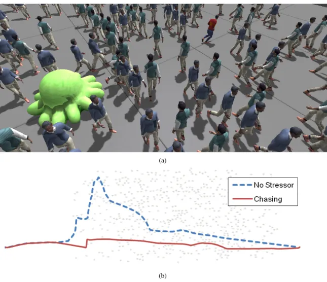
a fire stressor and crowding stressors. . . 30 2.5 Chasing scenario. (a) A red shirted agent is chased through a crowd by a
green monster causing a positional stressor. (b) If not being chased (dashed line), the agent’s path drifts as it navigates through the crowd. With our model, the agent takes a faster, more direct path through the crowd (red
line). This aggressive behavior is due to the effect of the stressor. . . 31 2.6 Comparison of simulated crossing speeds and real-world data. The less
time left to cross, the faster agents move. . . 32
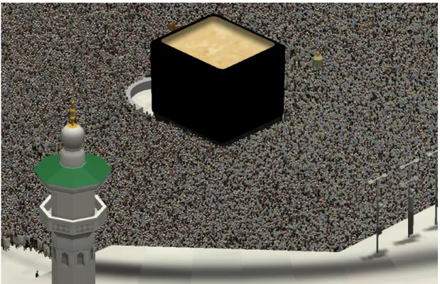
3.1 Simulation of Tawaf: We simulate pilgrims performing the Tawaf ritual. In our scene, about 35,000 agents circle around the Kaaba, performing a short prayer at the starting line while some of the agents try to get towards the Black Stone at the eastern corner of Kaaba. We model the interactions between the agents in a dense crowd, such as when the agents are pushed
by crowd forces (see video). . . 34 3.2 Wall Breaking. We demonstrate the physical forces applied by cylindrical
agents to breakable wall obstacles. Our algorithm can model such interac-tions between the agents and the obstacles in dense scenarios at interactive
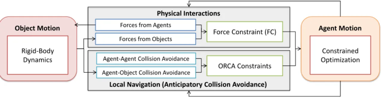
rates. . . 36 3.3 System Overview.The motions for objects and agents are computed by
a rigid-body dynamics solver and a constrained optimizer, respectively. Physical interactions between agents and obstacles determine forces. For obstacles, the forces serve as inputs to the rigid-body system; for agents, they become force constraints. These force constraints are combined with
the original ORCA planning constraints and serve as inputs to optimization algorithm. 39 3.4 Overview of FSM-based behavior modeling FSM states are used to
specify a set of available actions, along with the parameters used for physics-based interaction and local collision avoidance. Transitions be-tween the FSM states are made based on the result of our physical
interac-tion model combined with local collision avoidance method. . . 47 3.5 Rushing through still agents: The red agent tries to rush through a group
of standing agents, simulated (a) with only anticipatory collision avoidance and (b) with physical interactions. Using our method, the forces are
3.6 Two bottlenecks scenarioWe simulate and compare crowd behavior at two narrow bottlenecks, which are marked with red dotted lines. Bottle-neck (1) is barely wide enough for one person to pass through; bottleBottle-neck (2) is about twice that width and allows two agents to pass through it at a time. The result from collision-avoidance-only simulation results in an arch-shaped arrangement of agents in the crowd (highlighted with a yellow circle), which causes congestion at the bottleneck. Our method breaks the
congestion by allowing the agents to push one other in congested conditions. . . 50 3.7 Wall Breaking Simulations with Different Wall Properties. (a) When
the blocks are tightly attached, the wall is not broken. Instead, it is moved and rotated by crowd forces, and made a gap for the crowd to escape through. (b) When the wall consists of much heavier blocks, it does not break or move easily even after all the crowds (1200 agents) entered the isle. In this example, sometimes crowd makes a wave-like movement
where sparse density crowd movement is propagated front to back and vice versa. . . . 51 3.8 FSM for Dodge-ball ScenarioWe use a simple two-state FSM to specify
the game rule. The states consists of defense state and an attack state. During the attack-state, the character chases a ball and kicks it to its opponent. A character in defense-state tries to avoid the ball until the ball fell down on the ground. State transitions occur based on the location of
the ball and the kicking (applying force to the ball) action performed by the character. 52 3.9 Behavior examples modeled by our method(a) Green character
(user-control, left) kicks the red ball to the orange character (computer (user-control, right). Orange character is in the defense-state at that moment, and tries to avoid the ball. (b) When the ball falls down, the orange character’s state is changed to the attack-state. Collision avoidance behavior is changed just to meet non-overlapping condition with the ball and the character’s preferred velocity is updated towards the ball. The orange character approaches the
ball and kicks the ball to the green character. . . 53 3.10 Agent States and Transitions. The Tawaf states are represented as blue
circles and transition condition between these states are marked with arrows. We associate different properties like walking speed, pushing
condition, etc., with the agent behavior. . . 56 3.11 Density from the Simulated Result. Reported densities on the Mataf
floor can be as high as 8people/m2(Curtis et al., 2011); our method gives
a maximum density around 7.4agents/m2. . . 57 3.12 Pushed by crowd. Green circles represent the agents in the queue waiting
3.13 Region Speed from the Simulation ResultAverage speed of each region of the Mataf area. It matches the overall trend corresponding to higher average speed (region 6) and lower speeds (regions 1 and 6) observed
by (Koshak and Fouda, 2008). . . 59 3.14 Comparison of average region speeds. Blue bars correspond the average
speeds of the agents in each region when we introduce excessive pushing behavior to the exiting agent and queuing agents. Red bars correspond the average speeds when only the queuing agents pushes forwards while moving towards the Black Stone. Increasing number of pushing behaviors
brought a 20% to 40% increase in average speed. . . 60 3.15 Number of constraint optimization failures. We analyze the stability of
our method by measuring the number of constraint optimization failures. At the peak of congestion in the simulation, 95% of the agents are able to find velocities that satisfy all their constraints. Importantly, this stability holds across a variety of timesteps. As the timestep size varies from 0.01
up to 0.2, most of the agents are still able to find constraint-satisfying velocities. . . 61
4.1 (a)RVO Simulation Overviewshows agent A’s position (p), preferred velocity (vpref) and actual velocity (v), along with a neighboring agent B
(both represented as circles). If the ORCA collision-avoidance constraints prevent an agent A from taking its preferred velocity, as shown here, the actual velocity will be the closest allowable velocity. Taken together, these elements form an agent’s RVO statex. (b)Agent State EstimationAs new data is observed (blue dot) BRVO refines its estimate of a distribution of likely values of the RVO states (dashed ellipse). These parameters are
then used with RVO to predict likely paths (as indicated by arrow). . . 67 4.2 Overview of the Adaptive Motion Model. We estimate current statex
via an iterative process. Given noisy data observed by the sensor, RVO as a motion model, and the error distribution matrixQ, we estimate the current state. The error distribution matrixQis recomputed based on the difference between the observed state and the predictionf(x), and is used
to refine the current estimation ofx. . . 71 4.3 Benchmarks used for our experiments(a) In the Campus dataset,
stu-dents walk past a fixed camera in uncrowded conditions. (b) In the Bot-tleneck dataset, multiple cameras track participants walking into a narrow hallway. (c) In the Street dataset, a fixed camera tracks pedestrian motion on a street. (d) In the Students dataset, a fixed camera tracks students’
motion in a university. . . 75 4.4 Comparison of Error on Campus Dataset. BRVO produces less error
than Constant Velocity and Constant Acceleration predictions. Addition-ally, BRVO results in less error than using a static version of RVO whose
4.5 The effect of the EM algorithm. (a) This figure shows the trajectory of each agent and the estimated error distribution (ellipse) for the first five frames of Campus-3 data. The estimated error distributions gradually reduces as agents interact. For two highlighted agents (orange and blue), their estimated positions are marked with ’X’. (b) The improvement pro-vided by the EM feedback loop for various amounts of noise. As the noise
increases, this feedback becomes more important. . . 84 4.6 Path Comparisons These diagrams shows the paths predicted using
BRVO, Constant Velocity, and Constant Acceleration. For each case, ground-truth data with 0.05m noise, 0.1m noise and 0.15m are given as input for learning (blue dotted lines in shaded regions). BRVO produces
better predictions even with a large amount of noise. . . 86 4.7 Mean prediction error (lower is better).Prediction error after 7 frames
(2.8s) on Campus dataset. As compared to the Constant Velocity and Con-stant Acceleration models, BRVO can better cope with varying amounts
of noises in the data. . . 87 4.8 Prediction Accuracy (higher is better)(a-c) Shows prediction accuracy
across various accuracy thresholds. The analysis is repeated at three noise levels. For all accuracy thresholds and for all noise levels BRVO produces more accurate predictions than the Constant Velocity or Constant Acceleration models. The advantage is most significant for large amounts
of noise in the sensor data, as in (c). . . 88 4.9 Error at Various Densities (lower is better). In high-density
scenar-ios, the agents move relatively slowly, and even simple models such as constant velocity perform about as well as BRVO. However, in low- and medium-density scenarios, where the pedestrians tend to move faster, BRVO provides more accurate motion prediction than other models. KF fails to quickly adjust to rapid speed changes in the low-density region, resulting in larger errors than other methods. In general, BRVO performs
consistently well across various densities. . . 89 4.10 Error vs Sampling IntervalAs the sampling interval increases, the error
of Constant Velocity and Constant Acceleration estimations grows much larger than that of KF or BRVO. BRVO results have the lowest error among
the four methods.. . . 90 4.11 Comparison to State-of-the-art Offline MethodsWe compare the
av-erage error of LIN (linear velocity), LTA, ATTR, KF and BRVO. Our method outperforms LTA and ATTR, with an 18-40% error reduction rate over LIN in all three different scenarios. Significant improvement is made; compare the 4-16% and 7-20% error reduction rate of LTA and ATTR over
4.12 Kinematic model of the robotThe robot is modeled as a simple car at position(x, y)and with orientationθ. φis a steering angle andLis a
wheelbase. Our robot has the wheelbaseL= 1m. . . 94 4.13 Performance of the robot navigationWe measured the percentage of the
trajectories in which the robot reached farther than halfway to the goal position without any collision during the data sequence, using only GVO (blue bars), GVO with KF (red bars), and GVO with BRVO (green bars), both with 15cm sensor noise. In many of these scenarios, using GVO for navigation often caused a robot to stop moving through the crowd to avoid collisions (the freezing robot problem). GVO-KF shows lower performance in very sparse scenario, but outperforms GVO-only method as the number of pedestrians increases. GVO-BRVO algorithm further improves the navigation, especially for more challenging scenarios with
more pedestrians. . . 95 4.14 Example robot trajectory navigating through the crowd in Students
dataset. Blue circles represent current pedestrian positions, red circles are the current position of the robot, and orange dotted lines are the previous
positions of the robot. . . 96
5.1 Interactive data-driven simulation pipeline:Our method takes extracted trajectories of real-world pedestrians as input. We use the Bayesian infer-ence technique to estimate the most likely state of each pedestrian. Based on the estimated state, we learn time-varying behavior patterns. These behavior patterns are used as behavior rules for data-driven simulation and can also be combined with other multi-agent simulation algorithms. All
these computations can be performed in tens of milliseconds. . . 102 5.2 Pedestrian Dynamics Learning: A one-frame example from thezara01
dataset: (a) input consists of the manually-annotated trajectories (green) from the video; (b) probabilistic distributions of entry points at one frame, computed using the Gaussian Mixture Model (shown as elliptical regions); and (c) movement flows grouped by the characteristics of pedestrian
dy-namics, in which each grouping is represented by the same color. . . 107 5.3 Manko scenario: We highlight the benefits of entry point and movement
flow learning. (a) A frame from a Manko video, which shows different flows corresponding to lane formation (shown with white arrows); (b) and (c) We compute collision-free trajectories of virtual pedestrians. For (b), we use random entry points for virtual pedestrians and goal positions on the opposite side of the street. White circles highlight the virtual pedestrians who are following the same movement flow as neighboring real pedestrians. For (c), we use TVPD (entry point distribution and movement flow learning) to generate virtual pedestrians’ movement. The
5.4 Marathon Scenario:We compare the performance of different algorithms used to generate the trajectories of500pedestrians in the Marathon sce-nario: (a) The original video frame with18extracted trajectories (white); (b) A multi-agent simulation using five intermediate goal positions along the track; (c) We run the same simulation with optimized parameters using an offline optimization method; and (d) Instead of the intermediate goals and/or optimized parameters, we use only TVPD. Notably, TVPD captures
the pedestrian flow in the original video. . . 111 5.5 (a) A frame from a video of pedestrians in a street with extracted
trajecto-ries (shown in red); (b) Our simulation algorithm computes collision-free trajectories of virtual pedestrians (shown in blue) in the 3D virtual envi-ronment, which have the same movement flows as extracted trajectories
(red) . . . 115 5.6 ATC Shopping Mall Scenario:The real pedestrian trajectories are
com-puted using a 3D range sensor. (a) We show the flows highlighted with different colors in the original data. (b) We populate the scenario with 207virtual pedestrians. The virtual pedestrians exhibit the characteristics
observed in the original data. . . 116 5.7 Black Friday Shopping Mall scenario: (a) We use six simple
trajecto-ries generated in an empty space. (b) and (c) We create a new layout by adding obstacles interactively, and also increase the number of pedestrians in the scenario. (b) has 271 pedestrians, (c) has the twice higher number
of pedestrians generated at the same rate. . . 117 5.8 Crossing Explosion Scenario: (a) Initially, virtual pedestrians follow
the TVPD computed from the extracted trajectories. (b) The user places an explosion during the simulation. The pedestrians who perceive the
LIST OF ABBREVIATIONS
BRVO Bayesian-RVO
ORCA Optimal Reciprocal Collision Avoidance PDL Pedestrian Dynamics Learning
CHAPTER 1 Introduction
1.1 Motivation
The problem of understanding and modeling how a human crowd would behave in different situations arises in many areas. For example, during the planning stages, city, traffic, and evacuation engineers use crowd behavior modeling to predict the flows and usage pattern to evaluate their designs. Many other applications, including virtual reality, computer animation, games, and training, also need the capability to simulate the trajectory of pedestrians as well as the crowd behaviors. These applications require not only a realistic rendering of the virtual environment, but also realistic simulations of virtual crowds that become an essential element for an immersive user experience.
Human crowd behavior is often understood and modeled in two ways - macroscopic view, which looks at overall crowd behavior as a whole, and microscopic view, which looks at individual level behaviors and their interactions (Al-nasur and Kachroo, 2006). In a macroscopic view, human crowds generally exhibit a collective and structured formation. However, when we look at individual behav-iors, we see many variations depending on various factors such as the person, time, or environment. Currently, it is very challenging to simulate wide variety of crowd behaviors in virtual environments due to following reasons. First of all, there is no known mathematical model or algorithm that can describe all aspects of crowd behaviors. Psychologists and social scientists have proposed many different hypothesis about human behavior. Biomechanics have studied how physical conditions, including the terrain and obstacles, can affect human movement. It is important to model these biomechanical and psychological variabilities and conditions.
are interacting with other pedestrians. In a dense crowd, if a person pushes someone by mistake, the pushing force might be propagated through the crowd and thereby causes a domino effect. In extremely dense crowds, the forces from crowds sometimes become very large and can completely change the trajectory of an agent or make them fall. In these cases, crowd disasters can occur (Still, 2013). As the density of the crowd increases, it is more likely that even small motions can cause physical interactions with neighboring agents. For these reasons, understanding and simulating interaction between agents is necessary to simulate and analyze crowd scenarios.
As well as the problem of modeling the variations and interactions of crowds, designing a plausi-ble crowd scenarios can be another challenging and important proplausi-blem. In many applications, the goal is to generate trajectories of individual walking humans that match with real human movement and display emerging behaviors observed in real-world crowds. For these applications, there are many important problems to solve – such as a local interaction model for individual microscopic level behaviors, a higher-level behavior model that controls local behaviors and determines a macroscopic shape of crowd, and an interface to design the scenario. The solution for these problems should work well individually and also when combined together.
Last but not least, the simulation should be numerically stable and efficient. We often need to simulate dense, sometimes even massive (thousands to tens of thousands of agents in) crowds. The simulation should provide stable results in such cases, and be efficient enough to run at interactive rates for games, virtual reality, and computer-generated animation. Moreover, stability and efficiency in crowd simulation can also benefit applications in other areas outside computer graphics, such as robot navigation, real-time crowd tracking and scene analysis in computer vision.
1.2 Crowd Simulation
et al., 2006). These methods are able to simulate a large number of agents, but it is hard to control behavior of individual agents or small groups of agents. Agent-based techniques model interactions between the agents, mainly collision avoidance behavior. Force-based methods (Helbing and Molnar, 1995) use various forces to model attraction and repulsion between the agents; vision-based technique models steering behavior as a response to visual information (Ondˇrej et al., 2010). Other techniques model collision avoidance behavior using velocity-space reasoning (Karamouzas and Overmars, 2012; van den Berg et al., 2011). Among these techniques, we use the Optimal Reciprocal Collision Avoidance (ORCA) algorithm (van den Berg et al., 2011), which is based on a velocity-space reasoning, to simulate the local navigation of each agent. We use the termlocal behaviorto refer to the local navigation behaviors that models interactions with nearest neighbors.
1.2.1 Local Collision Avoidance in Velocity-Space Reasoning
We briefly summarize ORCA algorithm that we use as an underlying multi-agent simulation technique to model individual goals and interactions between people. We chose a velocity-space reasoning technique based on ORCA (van den Berg et al., 2011), which implements an efficient variation of Reciprocal Velocity Obstacles (RVO) (van den Berg et al., 2008a).
ORCA uses a set of linear constraints on an agent’s velocities in order to ensure that agents avoid collisions. The constraints are represented as the boundary of a half plane containing the space of feasible, collision-free velocities calledpermitted velocities. Agents are assumed to have a preferred velocity, which is the velocity at which the agent would travel if there were no collisions to avoid. At each timestep, an agent computes a new velocity that satisfies the velocity constraints, then updates its position based on the new velocity. See (Curtis and Manocha, 2012) for the various benefits of using velocity-based reasoning for crowd simulation. RVO-based collision avoidance has previously been shown to reproduce important pedestrian behaviors such as lane formation, speed-density dependencies, and variations in human motion styles (Guy et al., 2010, 2011).
1.2.2 Modeling Local Interactions
These algorithms provide a general formulation that can be used for every agent in the environment. However, when all the agents exhibit the same behavior patterns, the resulting simulation can look unnatural since it does not capture variations of individual behaviors that we can observe in the real-world. (Peters and Ennis, 2009; Praˇz´ak and O’Sullivan, 2011) study the perceptual effect of variation of crowd behaviors and different size of groups in crowd simulation. Lerner et al. point out the restricted number of behavior rules as one of the limitations of crowd simulation algorithms and propose an example-based method to add a variety of behaviors (Lerner et al., 2007).
Some agent-based methods approach this problem by defining different behavior rules to multiple groups of agents. For example, Yeh et al. describe the geometric notion of a composite agent, which can model different behaviors including aggression, social priority, authority, protection, and guidance (Yeh et al., 2008). Pelechano et al. simulate different wayfinding behaviors of trained/untrained leaders and the followers in emergency situations (Nuria Pelechano, 2005). These behavior patterns are chosen based on a given role, and may not change during simulation. More recently, methods based on psychological theories have been proposed. Pelechano et al. define behavior rules for five different types of personalities (Durupinar et al., 2011). Guy et al. use personality trait theory to model heterogeneous crowd behaviors (Guy et al., 2011). Curtis et al. propose an asymmetric collision avoidance method that can handle some limitations from prior symmetric collision avoidance techniques (i.e., where each agent compute collision avoidance behavior in the same way as other agents) (Curtis et al., 2012b).
repulsive force (Yu and Johansson, 2007). Curtis et al. use velocity-space collision avoidance technique to model dense crowds performing a religious ritual (Curtis et al., 2011).
1.2.3 High-level Behavior Modeling
Higher-level behavior models provide a way to control local navigation and collision avoidance behaviors of agents. Unlike local interaction behaviors, which can be modeled with mathematical formulations, higher-level behaviors can hardly be formulated due to the complexity of human behaviors. Instead, it has been a common practice to script or manually specify behavior rules. For example, cognitive approaches focus on defining rules or behavior to mimic cognition or the decision making process of the crowd (Shao and Terzopoulos, 2005; Ulicny and Thalmann, 2002). These methods can simulate very specific and detailed behaviors when used with corresponding scenarios such as buying a ticket or waiting in line. Also, Finite State Machine (FSM) has also commonly used to encode procedural behaviors or set of goals based on an agent’s state (Bandini et al., 2006; Paris and Donikian, 2009; Sean Curtis, 2013).
On the other hand, data-driven or example-based crowd simulation algorithms synthesize behav-iors from real-world behavior examples. Some higher-level behavbehav-iors, such as formations or group behaviors, are implicitly exhibited from the examples, rather than explicitly specified behavior rules. Motion capture or real-world trajectory data are commonly used source of examples. For example, trajectory data extracted using semi-automatic trackers are used to generate group behaviors (Lee et al., 2007), and extended to build group formation models (Ju et al., 2010). Populating the virtual scenes can be done by copying and pasting small pieces of synthesized motions (Li et al., 2012; Lee et al., 2006; Kim et al., 2012a; Shum et al., 2012). The emergence of data-driven methods grows out of the increasing availability of real-world datasets of individual humans and crowds, driven in part by improvements in high-resolution cameras and motion-capture systems.
1.2.4 Crowd Simulation for Robotics
Robots are becoming increasingly common in everyday life. As more robots are introduced into human surroundings, it becomes increasingly important to develop safe and reliable techniques for human-robot interaction. Robots working around humans must be able to successfully navigate to their goal positions in dynamic environments with multiple people moving around them. A robot in a dynamic environment thus needs the ability to sense, track, and predict the position of all people moving in its workspace to navigate complex environments without collisions.
Sensing and tracking the position of moving humans has been studied in robotics and computer vision, e.g. (Luber et al., 2010; Rodriguez et al., 2009; Kratz and Nishino, 2011). These methods often depend upon an a priori motion model fitted for the scenario in question. More recently, local collision avoidance models have been used for pedestrian tracking algorithms (Pellegrini et al., 2009; Yamaguchi et al., 2011). Multi-agent interaction models effectively capture short-term deviations from goal-directed paths. However, in order to do so, they must already know each pedestrian’s destination; they often use handpicked destination information, or other heuristics that require prior knowledge about the environment. As a result, these techniques have many limitations: they are unable to account for unknown environments with multiple destinations, or times when pedestrians take long detours or make unexpected stops.
1.3 Thesis Statement
Our thesis statement is as follows:
Velocity space planning can be enhanced by incorporating modeling of human behaviors using
psychological, physics-based and pedestrian dynamics learning principles, and these models can
each be combined to provide plausible crowd behavior for interactive applications and robotics.
Overall Crowd Behaviors and High-level Behaviors
Crowd Trajectory-Behavior
Characteristics Learning and Analysis (Chapter 4 and Chapter 5)
Dynamic, Heterogeneous Behavior Model
(Chapter 2)
Crowd Trajectory Behavior Individual Differences Collision Avoidance Result
Physical Interaction Model +
Local Navigation Algorithm (Chapter 2)
Figure 1.1: Components in Crowd Sim (colored outline) as related to techniques (rounded rectangles) used in this thesis.
1.4 Main Results
Figure 1.1 visualizes how each chapter in this thesis is related to crowd simulation as a building block. As highlighted in the thesis statement, the techniques are based on psychology, physics, and learning principles. These can cover individual differences, local navigation, and high-level behavior learning, respectively.
Dynamic, Heterogeneous Crowd Behaviors: We present a method to simulate dynamic patterns and variations of individual behaviors based on psychological theories. Our method can handle spatially- and temporally-varying situational factors in a unified framework and can generate several emergent behaviors in different scenarios that match real-world observations.
Physical Interaction Models:We present a technique to model various interactions involving physical contacts, such as collision response and intentional physical interactions. Our method handles physical interactions while still preserving the ability of the crowd to avoid collisions with each other. In addition, agent-object interactions and agent-user interactions are performed at interactive rates using our approach. Our formulation can be useful for games, augmented reality or virtual reality applications, where the user can directly interact with other virtual agents or the objects in the scene.
Adaptive Motion Model: We present a method to improve the motion model by learning from real-world trajectory data generated using the sensors. Our approach is able to learn individual characteristics in an online manner, without any prior knowledge to the scene. We use the results to predict the motion of the individuals in the scene, and this can be used to improve the quality of the interactions between the users and the computer system for human-computer interactions, human-robot interactions, computer tracking applications, or augmented reality.
Interactive Data-driven Crowd Simulation: We present a method to learn high-level crowd behaviors from real-world data. Our method retains some of the advantages of data-driven methods that use trajectory patterns from real-world data, but no longer requires building large database or pre-processing of the input data. Also, our method can be used with agent-based simulation techniques without specifying complex behavior rules. Our method can handle both structured and unstructured crowd behaviors, with temporal/spatial behavior changes.
1.4.1 Modeling Dynamic, Heterogeneous Behaviors
(a) Initial Approach (b) Lane Formation (c) Alarm Response
Figure 1.2: Opposing Group scenario. (a) Two opposing groups approach each other. (b) Agents initially form natural lanes. (c) After experiencing stress from the alarm the lane formation breaks down into uncooperative, clogged and congested behavior.
Sometimes designers can carefully adjust simulation parameters to model different crowd behaviors that fit to a specific scenario, but the process can be time-consuming.
Our approach is based on observations and understandings from psychology literature. We define a general motion model to describe the variability and the dynamic changes of individual behavior. Our method is based on Attribution theory, that finds a cause of a behavior from a dispositional attributes and situational attributes. Dispositional attributes are internal factors such as personality, and situational attributes are external factors such as stimulus from current situation (Heider, 1982). For example, a very polite, patient person who yields others for a way, but might show aggressive pushing behavior towards the other people in a building with a fire.
As a first step, Guy et al. proposed a mapping between simulation parameters and personality space of the virtual agents, acquired from a user study (Guy et al., 2011). This enables us to simulate agents with different personalities. In Chapter 2, we propose a model that takes account situational stimuli. The agents perceive stimuli from current situation and respond dynamically based on their perceived amount of stress. Our resulting system generates different behaviors of an agent ranging completely based on their personality when they are not exposed to any external stimuli, to a behavior under maximum stress when their accumulated stress reaches threshold.
with other models and reproducing empirical data collected from the real crowd, and to show that the resulting behavior conforms psychology theories, such as Yerkes-Dodson’s Law (See Fig. 1.3).
Figure 1.3: Average speed of agents in the Opposing Groups scenario at various levels of stress. The Yerkes-Dodson Law states that stress should increase performance up to a point then decrease it, a result which is matched by the proposed model.
1.4.2 Modeling Physical Interactions
Most of the multi-agent simulations focus mainly on local collision avoidance. These techniques model agent’s behavior by defining how they will perceive or acquire knowledge about impending collisions, and how each of them will respond (change their behavior) to avoid impending collision. In other words, it is expected from an agent with a certain level of intelligence that when they see other agents or obstacles on their way to the destination, then they should take a detour for safe navigation. However, very little attention was given to the behavior of an agent when collision actually happens, though such situation is observed frequently in real world, especially in dense settings. We can easily imagine some people who are pushed by somebody in a hurry, for example, in a crowded subway station. Moreover, many other interactions are initiated by contact, that is by physically touching or applying force to a person or an object.
motion. For example, we can model balance-recovery motion of the agents, or a propagation of a force or a motion after the interaction through nearby agents in a dense crowd. Moreover, our method is able to handle both collision avoidance and physical interactions with dynamic obstacles (e.g., movable rigid-bodies), as opposed to the previous techniques only considered static obstacles.
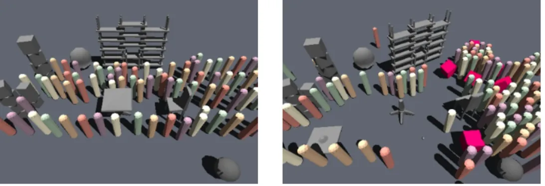
Our method provides a numerically stable and fast simulation of a large (a few thousands), dense (up to 7-8agents/m2) crowd. Since our method is able to handle dynamic obstacles interacting with the agents, and is fast enough for real-time interactive simulation, users can participate in the simulation by moving rigid bodies inside the scene. This movement dynamically changes the environment for the moving agent. Fig. 1.4 shows an example scenario that consists of several pieces of furniture and 1200 agents. In combination with the Bullet Physics library (AMD, 2012), we were able to simulate complex interactions between agents and dynamic obstacles in the environment.
Figure 1.4:Interactive Simulation of Physical Interactions between Agents, Furniture in Office, and User-thrown Obstacles. Agents navigate to avoid office furniture (left). As users insert flying pink boxes into the scene, the agents get pushed, collide into each other, and avoid falling objects (right).
We extend the physical interaction model by combining with Finite State Machines (FSM) to model high-level behaviors involving decision making process. In addition, we we have simulated real world examples of massive crowd such as those in the Tawaf ritual. Our method was able to generate many emergent behaviors compared with real-world behaviors.
1.4.3 Adaptive Motion Model: Learning Individual Motion Parameters from Real World Crowd
for each individual that can best describe the observed motion trajectory. We present an online, individualized and adaptive system that learns behavior parameters and evolves itself as it gets more observations. The fitted motion model can be used to predict the motion of each individual in the near future (a few seconds to a few minutes), and can be used for virtual reality, augmented reality, human-robot interactions, or tracking applications.
Our approach has unique properties and benefits compared to prior approaches. First, our method can learn unique characteristics of each individuals. Prior techniques find a global, uniform parame-ters for everybody during the entire sequence of data. Instead, we learn time-varying parameparame-ters for each individual, which preserves individual characteristics. Second, our method can generate better representation of time-varying changes of motion by adapting itself to the new observations. We use maximum likelihood estimation technique to improve the accuracy of the motion model. Thus, our method provides better local prediction at a certain time, also resulting in increased overall accuracy for the entire sequence. Finally, our method does not need prior knowledge about the scene and can be used to learn and predict online. Note that prior approaches require manual work or preprocessing to find a global parameters from the same scenario.
We perform series of experiments to demonstrate the performance of the proposed method. The method performs very well with varying number of individuals, varying noise level, scenarios with varying density (low-high), and sparsely sampled data (sampled every 0.4 - 1.6 seconds). Moreover, we extend the prediction method for a robot navigation problem and show the performance improvement.
1.4.4 Time-varying Crowd Behavior Learning for Crowd Simulation
(a) (b)
(c) (d)
CHAPTER 2
Interactive Simulation of Dynamic Crowd Behaviors using General Adaptation Syndrome Theory
2.1 Introduction
Simulating the wide variety of behaviors seen in real-world crowds is important for many inter-active applications, including games and virtual environments. There are no known computational models that can simulate different types of crowd behaviors. At a broad level, crowd behaviors are governed by the characteristics of the individual humans and the surrounding environment.
Psychologists have extensively studied human characteristics and behaviors. Differences in human behaviors are governed by multiple factors, including differences in stimuli, genetic endow-ment, physiological state, cognitive state, social environendow-ment, cultural environendow-ment, previous life experiences, and personal characteristics (Eysenck, 2002). Despite this diversity, factors affecting human behaviors can be categorized into some basic types.
Attribution theory, for example, divides these causes into dispositional attributes and situational attributes. Dispositional attributes capture internal factors such as personality or characteristics, while situational attributes capture external factors such as current situation (Heider, 1982). Cattell (Cattell, 1952) suggested a similar divide in the causes of behavior termedpersonalityandsituational factors.
(a) Crossing immediately before light change (b) Crossing after red light
Our proposed technique for simulating dynamic crowd behaviors is based on this dichotomy, and we use separate models for an agent’s personality and another one to account for situational factors.
In crowd simulation literature, techniques to model heterogeneous behaviors using personality models have been proposed (Durupinar et al., 2011; Guy et al., 2011). Resulting simulations can successfully generate a variety of behaviors happening in a scene, but may not be able to model dynamic behaviors. These dynamic behaviors correspond to changes in individual and crowd behaviorsin response to a situation. For example, a calm or composed person walking through a pedestrian crossing may become aggressive when the light turns red from green. Similarly, the same person may cut through a crowd when a train approaches the platform at a train station. The dynamic nature of human and crowd behaviors is also observed during fearful or panicked situations, such as fire evacuations, where individuals change behaviors in response to emergencies and alarms.
Our objective is to model such dynamic crowd behaviors at interactive rates. We model these behaviors as a reaction to meet certain demands or cope with the changes in a situation or environment. These situational factors will be referred to asstressors, and the effect of these stressors on the agents will be measured asstress. Our approach is build on the psychological theory of General Adaptation Syndrome (Selye, 1956) that provides a well-established behavior model of how humans react to stress.
Main Result: We present a new technique to simulate dynamic patterns of crowd behaviors by considering various types of stressors. Our model accounts for both stable, consistent aspects of behaviors, influenced by personality, and the dynamic changes in behavior due to situational factors. Our main contribution is a method that incorporates well-established psychological models of stress into crowd simulation. Our algorithm generates realistic, dynamically-changing crowd behaviors based on a few high-level parameters that model how individuals vary in their response to stress.
The resulting simulation shows a variety of dynamic crowd behaviors under stress, such as cutting through the crowds, walking with variable speeds, and breaking lane-formation over time or in different situations. We perform both qualitative and quantitative comparison between our simulation results and real-world observations. Our method has a small computational overhead and can simulate thousands of agents responding to dynamic stressors in real time on a single-core CPU.
The rest of this chapter is organized as follows. Section 2.2 provides an overview of related work both from crowd simulation and psychology. Section 2.3 gives an overview of psychological models and of our approach. Section 2.4 discusses our approach to modeling stress accumulation. Section 2.5 presents the overall dynamic crowd simulation algorithm. We highlight the results in Section 2.6. We direct the readers to the project webpage (http://gamma.cs.unc.edu/GAScrowd/) for the videos as well as the related publication (Kim et al., 2012c).
2.2 Related Work
In this section, we give a brief overview of prior work from both psychology and crowd simulation literature. Our discussion here focuses on modeling dynamic behaviors due to stress. For a broader coverage of human psychology, we refer the reader to Eysenck (Eysenck, 2002).
2.2.1 Stress
Several researchers have attempted to characterize how humans respond to stress in terms of both internal, physiological changes and external, behavioral changes. Early attempts to model how human behavior changes in different situations include the work of Cattell (Cattell, 1952), who proposed a mathematical formula to predict human behavior as a function of personality and situation. More recently, Leon (Leon, 2010) have extended this work to the pedestrian behavior, modeling the increased aggression people exhibit when stressed.
stress and aggression has been particularly well established (Evans, 1984; Anderson, 2001; K.B. and Rasmussen, 1979) and holds across a variety of stressors (Berkowitz, 1990; Miller, 1941).
2.2.2 Crowd Simulation
The area of crowd simulation and multi-agent navigation is an active area of research, with a wide variety of methods and results. We primarily focus on interactive methods for modeling crowd behaviors. For a broader coverage of the field we refer the reader to a recent survey (Pelechano et al., 2008).
2.2.2.1 Interactive Crowd Simulation
There are several frameworks proposed for simulating and rendering large number of crowds. The Virtual Dublin project simulated crowds in an urban simulation at interactive frame rates (Dobbyn et al., 2005). Yersin et al. (Yersin et al., 2009) proposed a method using pre-computed crowd patches to populate a large-scale virtual environment for real-time simulations. Parallel GPU-based algorithms have also been proposed for both crowd simulation and high-quality rendering (Shopf et al., 2008).
Many real-time techniques have also been suggested for goal-directed multi-agent simulations. Among them the HiDAC system is able to simulate various behaviors (Pelechano et al., 2007). Recip-rocal Collision Avoidance based methods have been successfully applied to simulate crowds (van den Berg et al., 2011). Patil et al. (Patil et al., 2011) proposed an interactive algorithm based on navigation fields, where users can directly control the crowd movement.
2.2.2.2 Behavior Modeling
Rule-based approaches are commonly used to model complex behaviors. These include frame-works based on motor, perceptual, behavioral, and cognitive components for modeling pedestrian behavior (Shao and Terzopoulos, 2005) and modeling decision-making process (Yu and Terzopoulos, 2007).
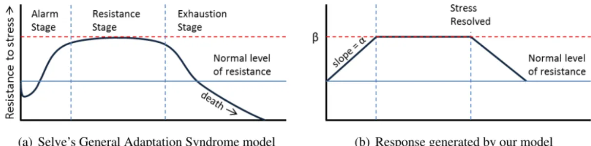
(a) Selye’s General Adaptation Syndrome model (b) Response generated by our model
Figure 2.2: General Adaptation Syndrome and approximation(a) GAS model of the human response to stress. After an initial disturbance, the resistance level increases up to maximum capacity. If the stress is unresolved, the resistance gets weaker and is no longer effective (causes illness or death). (b) Our approximation of GAS model. We assume acute stress, i.e. no exhaustion stage. Instead, agents are relieved from stress when the stress is resolved. The shape of the response is determined by the stress accumulation rateαand maximum capacityβ
.
of a composite agent, which can model different behaviors including aggression, social priority, authority, protection, and guidance.
Many researchers have used psychological factors in crowd simulation. Pelechano et al. (Nuria Pelechano, 2005) simulated different wayfinding behaviors of trained/untrained leaders and the followers in
emergency situations. These behavior patterns are chosen based on the given role, and may not change during simulation. Sakuma et al. (Sakuma et al., 2005) proposed a local collision avoidance method that switches discreetly between smooth and urgent avoidance behaviors based on the urgency of collisions. Nygren (Nygren, 2007) proposed a system which models the effects of psychological factors by using artist derived rules to change behaviors when the agents are fearful, fatigued or happy.
More recently, there have been attempts to create realistic, heterogeneous crowd behavior based on human psychology, especially personality traits (Guy et al., 2011; Durupinar et al., 2011). These approaches provide a way to model heterogeneous behaviors, but the behavior patterns do not change over time. Our approach builds on these works to model dynamic crowd behaviors.
2.3 Preliminaries and Overview
2.3.1 Psychological Models of Stress
There are multiple definitions of stress in psychology literature. In a broad sense, stress can be defined as any change caused by interactions between the environment and individuals. Generally, stress is caused by a discrepancy between environmental demands and the abilities of individuals (Cox, 1978). In other words, people become stressed when they feel they are challenged or they need to cope with the current situation. Stressors are what cause the stress, they can be a situation, an object, or even other individuals. There are a number of sources that cause stress. In this chapter, we focus on the following types of stressors:
1. loads given to individuals (challenging situations), e.g. time constraints associated with the goal of each agent;
2. perceived threats, e.g. fire, threatening animals or objects;
3. unpleasant events, e.g. heat, noise, air pollution (smoke, malodor), and over-crowding.
The emotional or behavioral effect of stress is generally associated with increased aggression. This link can be found is both psychological models of emotion (Berkowitz, 1990) and empirical studies of human behavior (Evans, 1984; Anderson, 2001) However, the result of stress is not always negative. In some situations increased aggression can have positive effects, and can improve performance up to a point (Yerkes and Dodson, 1908).
By measuring the connection between how people act (measured through recorded observation) and how people feel (measured indirectly via heart rate, skin temperature and self reporting) psychol-ogists have established a consistent relationship between increased stress and increased aggressive and impulsive behavior (Anderson, 2001). This result has held across various stressors, different settings, cultures, and genders (Evans, 1984; K.B. and Rasmussen, 1979). Our approach uses the result of these empirical studies to model various stressors and their effects as increasingly aggressive and impulsive crowd behaviors.
2.3.2 General Adaptation Syndrome (GAS)
model as a general response to any stressor (toxins, cold, injury, fatigue, fear, etc.) The GAS model has three stages of response: alarm, resistance, and exhaustion (see Figure 2.2(a)). When individuals perceive a stress, in the alarm stage, they ready themselves for ”fight” or ”flight”. In the resistance stage, they work to resolve the stress at their full capacity. If the stressor is not removed (i.e. a chronic stressor), they reach the exhaustion stage and resistance becomes ineffective.
Research shows that the GAS model also applies to various physiological changes and general activities (Eriksen et al., 1999). Additionally, there is a stable relationship between psychological response of how stress makes a person feel and the physiological response of how it changes their behavior (Mordkoff, 1964).
2.3.3 Approximation of the GAS Model
While the GAS model suggests the shape of a person’s stress responses, it does not provide quan-titative values for the level of response to different stressors. We propose a quanquan-titative approximation of the GAS model, which produces a stress response consistent with that model.
We first assume an agent is experiencing a perceived stress with a value ofψ. Our goal is to compute a stress response for an agent, denoted asS. This value will be a function of the perceived stress,ψ. To maintain consistency with the shape of the GAS response, our model has two main attributes. First, an agent’s change in stress response is capped by a maximum rate, denoted asα. This is to ensure that an agent’s stress response does not jump suddenly in response to a sudden stress. Secondly, an agent’s stress response is capped at some maximum amount, denoted asβ. This is to ensure that if the perceived stress increases unboundedly, there will be a limit on an agent’s response.
Taken together,αandβwill map the perceived stressψto a stress responseSas follows:
dS dt =
α ifψ > S
{−α≤ dψdt ≤α} ifψ=S
−α ifψ < S
(2.1)
Figure 2.2(b) shows the resulting stress response induced by a instantaneous, large value of ψ(which lasts until the stress is resolved). This is similar to the stress induced by a sudden, loud warning alarm sounding. The stress response, which results from Eqn.2.1, shows a similar shape to that corresponding the GAS model (shown in Figure 2.2(a)).
In general, an individual’s stress response (parameterized byαandβ) can vary between different people and across different situations. The values for these parameters can be chosen by an artist for a specific, potentially exaggerated effect (as discussed in Section 2.5.2) or chosen to match real-world data (as discussed in Section 2.5.3).
Our purpose is to provide a general framework that can simulate dynamically changing behavior triggered by stress response in real-time crowd simulations. To that end, we make some simplifying assumptions, notably, treating the parametersαandβ as constants, and a further assumption that agents will not be exposed to a stressor long enough to reach the exhaustion or death stage.
2.3.4 Overview of our Approach
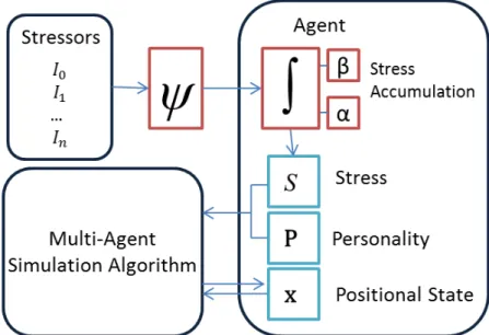
Our overall system has three main components. Firstly, the stressor provides a source of stress for the agents. Secondly, the stress accumulation function Eqn.2.1 which is determined by the GAS model. Thirdly, a multi-agent simulation algorithm that is capable of changing an agent behavior by increasing its aggressiveness and impulsiveness.
The interaction between a stressor and an agent’s perceived level of stress from that stressor is determined by theperceived stress function,ψ. The form of the perceived stress function varies based on the type of stress, and we highlight several examples in Section 2.4. The interactions between the agents are updated as a function of the accumulated stress,S. This aspect is discussed in Section 2.5. Figure 2.3 provides an overview of the system. In the next two sections we discuss details of how we model each component.
2.4 Modeling Stress and Stressors
Figure 2.3:System OverviewDifferent levels of stressed behaviors are simulated by updating agent parameters.
2.4.1 Perceived Stress
In order to define the perceived amount of stress experienced by an agent, we adapt Stevens’ psychophysical power law (Stevens, 1957). This law states the relationship between the perceived magnitude of a stress and the physical measurement of the stimulus intensity, e.g. the relationship between sound intensity and perceived loudness, luminance and perceived brightness, and density and perceived crowding.
Steven’s Law states that the relationship between the perceived intensity of the stressor,ψ, and the magnitude of the physical intensity of the stressor,I, has the form:
ψ(I) =kIn, (2.2)
Middlemist et al., 1976; Oswald and Bratfisch, 1969). Inpired by this observation, we use Eqn.2.2 as a generic model of the effect of the stressors.
2.4.2 Stressor Prototypes
We define four different prototype stressors, which can be used to model a variety of forms of stress. These are time pressure, positional stressors, environmental stressors, and interpersonal stressors.
Time pressure: These are stressors associated with an attempt to reach a goal by a particular time. Examples could include crossing the street at a timed light, boarding a train before the doors close, or evacuating a building during a fire.
To model these type of stressors, agents are given a goal position and a time constraint oftallowed.
We model the intensity of the time pressure,It, as a function of the difference between the allowed
time and the estimated arrive time. Formally:
It= max(testimated−tallowed,0), (2.3)
where testimated is the estimated amount of time an agent will take to reach its goal, i.e.
testimated=distRemaing/avgSpeed.
Area stressors: These are stressors that arise from a condition in the environment. Examples include noise, heat, bright lights, and smoke. The intensity of these types of stressors is almost constant over a area, that is
Ia=
c ifpa ∈A
0 ifpa ∈/ A
(2.4)
whereAis the area under effect from the stressor andpais the agent’s current position.
Formally, we define the intensity as
Ip =kpa−psk, (2.5)
wherepaandpsindicate the position of the agent and the stressor, respectively.
Some stressors, such as fire, have a high intensity over a large area. For these stressors, we use a Gaussian distribution with a standard deviation ofσto compute the intensity:
Ip=N(pa−ps, σ). (2.6)
Interpersonal stressors: These are stressors associated with the stress coming from other agents. A common example includes crowding, where some people feel stress due to too many people being too close. These interpersonal stressors have been found to follow a similar exponential law (Middlemist et al., 1976; Oswald and Bratfisch, 1969). We model these stressors’ intensity as a function of the difference between the preferred density of neighbors, and the actual density of neighbors:
Ii= max(ncur−npref,0), (2.7)
wherencur is number of current neighbors in a unit space andnpref is the preferred number of
neighbors in the same area.
2.4.3 Stress Model
Each of the above stressor prototypes define an intensityI which, when combined with Eqn. (2.2), is used to define the perceived stressψ. Given the currentψ, an agent’s stress response,S, is determined by Eqn. (2.1).
Multiple stressors:When exposed to multiple stressors, we compute a weighted sum of each stress value to find the total stress experienced by the agent. This model conforms with the discussion in Lazarus (Lazarus, 1993) that people selectively pay attention to the stimulus.
Formally, we define the total perceived stresssas
S=XωiSi, (2.8)
whereωiis the weight of each individual stressorSi. The values ofωican be chosen to weigh the
stresses equally or can be used to give priority to more important stressors.
2.5 Behavior Mapping
In Section 4, we defined our psychologically-motivated model of how an agent’s level of perceived stress, S, changes in response to various stressors. We now discuss how an agent’s behavior changes in response to these changes in the stress level.
As discussed in Section 2.3.1, the primary observable response to increasing levels of stress is an increase in aggressive and impulsive behavior. Our method for modeling the dynamic changes in behavior that arise from stress relies on a multi-agent system capable of simulating changes in the levels of aggression and impulsiveness displayed by the agents. We use the multi-agent simulation algorithm proposed by Guy et al. (Guy et al., 2011), though our methods could be easily applied to other approaches with similar capabilities.
2.5.1 Incorporation of Behavior Changes
agents sight distance. Different parameter values generate different goal-directed behaviors and local interaction with neighboring agents, which are perceived as personality.
They asserted that there are two primary dimensions (or principle components) of crowd behavior, and that these can be regarded as high-level parameters. The first, denoted PC1, was correlated to an increased level of of “extraverted” or more “intense” behavior from the agents. The second dimension, PC2, was associated with increasingly “careful” behavior. Using this parameterization, we are able to determine how to automatically select simulation parameters for the multi-agent modeling system to produce behaviors that appear to be as increasingly aggressive and impulsive. We denote this change in parameters as the stress behavior vector, Bstress since adding it to an agents current simulation parameters will increase their perceived level of stress. For the results in this chapter, we use
Bstress= (PC1 PC2)
0.95
−0.3
(2.9)
because it produces behavior which is predominately aggressive (very high “egocentricity”) and somewhat impulsive (negative “carefulness”).
2.5.2 Coupling with Personality Attributes
Guy et al. (Guy et al., 2011) also provided a matrix,Apc, which gives a linear mapping between
the values of PC1 and PC2 and the simulation parameters. The same work further suggested a matrix,Aadjwhich maps a variety of different personality descriptors to simulation parameters. We
determine the final behaviors of our agents as a linear combination of these two parameter matrices: the first representing an agent’s situational response and the second the agent’s stable personality. The effect of the situational response is scaled by the amount of perceived stresss¯that an agent is current experiencing.
The resulting equation for determining simulation parameters that depicting the agent’s behaviors due to inherent personality traits and dynamically changing stress response is