Sharif University of Technology
Scientia IranicaTransactions E: Industrial Engineering www.scientiairanica.com
The hierarchical hub covering problem with an
innovative allocation procedure covering radiuses
E. Korani
and R. Sahraeian
Department of Industrial Engineering, Faculty of Engineering, Shahed University, Tehran, Iran. Received 15 February 2012; received in revised form 12 December 2012; accepted 6 May 2013
KEYWORDS Hierarchical; Hub location; Hub covering; p-Hub median.
Abstract.Hub location problems deal with locating hub facilities at one level of services or one type of facility, but some systems are performed by several types of facility. So, this paper attempts to study a single allocation hierarchical hub covering a facility location problem over a complete network linking at the rst level, which consists of hub facilities known as central hubs. In addition, the study proposes a mixed integer programming formulation and nds the location of the hubs at the second level and central hubs at the rst level, so that the non-hub and hub nodes are allocated to the opening hub and central hub nodes. Thus, the travel time between any origin destination pair is within a given time bound. The current study presents an innovative method for computing the values of radiuses in order to improve the computational time of the model and to test the performance of the mentioned heuristic method on the CAB data set and on the Turkish network. Helpful results were obtained, including: severe reduction in the time of solution, rational distribution of the centers for presenting results, equality (Justice) and appropriate accessibility consistent with dierent levels of servicing. A computational experience was applied to the Iranian hub airport location.
c
2013 Sharif University of Technology. All rights reserved.
1. Introduction
The hub location problems deal with locating hub facilities and the assignment of demand nodes to them, and obtaining minimum total cost for network establishment. There are two types of allocation for links in hub networks: single assignment and multiple assignment. The former allocates demand nodes exactly to a hub and the latter connects non-hubs to one or more than one hub. The single assignment hierarchical hub location problem with two levels locates hub facilities at any level of hierarchy and allocates demand nodes to exactly one hub and one central hub, such that the travel time between any origin destination pair is within a given time
*. Corresponding author.
E-mail addresses: [email protected] (E. Korani), [email protected] (R. Sahraeian)
bound. Frequently, the routing costs between hubs and central hubs and between central hubs are discounted at a certain rate, in order to take the benets of economies of scale. Usually, in classical hub networks, hub facilities at the top level are connected to a complete network and at the second and third level links form a star network. These problems are applied to many elds, such as transportation (airline, cargo delivery), and telecommunication systems. Regarding the applied eld of the present problem and related problems, the following cases could be mentioned: a) Health care systems;
b) Solid waste management systems; c) Production-distribution systems; d) Education systems;
e) Emergency medical services (EMS); f) Telecommunication network systems;
Other relevant ones above have been examined by Sahina and Sural [1], which includes comprehensive research into hierarchical problems.
The hub location problem was presented by O'Kelly [2] with single allocation and minimizing total routing costs in a quadratic model formulation. This model has become the basis for all hub location prob-lems. O'Kelly illustrated 2 [0; 1] as the constant discount factor, in order to reect economies of scale in hubbing links. Among several research elds in the hub location problem, the main one is the linearization of the quadratic model introduced by O'Kelly [2], which was investigated by Aykin [3], Campbell [4], Ernst and Krishnamoorthy [5], O'Kelly et al. [6] and Skorin-Kapov et al. [7].
Following the same trend of conducted research, Campbell [4] presented a new version of the hub location problem, entitled the hub covering problem. The hub covering problem nds the location of a hub and allocates demand nodes to opening hub facilities, so that the travel time between any origin destina-tion pair is within a given time bound, and these problems have been presented with dierent objective functions. The hub covering problem presented by Campbell [4] created two new models for hub location problems (p-hub center & hub covering) with dierent objective functions. There are two types of hub covering problem: Hub set-covering that minimizes the cost of establishing the hubs for covering all demand nodes, and hub maximal covering that maximizes the non-hubs covered with a predetermined number of hubs. The mixed integer formulations for both problems are introduced by Campbell [8]. Kara and Tansel [9] studied the single allocation hub set-covering problem and demonstrated that it is NP-hard. They also presented a new linear model of their quadratic model. Wagner [10] proposed new formulations for hub covering problems in two situations of single and multiple assignment; these formulations need fewer numbers of variables and constraints compared to the Kara and Tansel [9] formulation. Ernst et al. [11] presented new formulations for the single and mul-tiple assignment hub set covering problem via as the covering radius. These formulations are better than Kara and Tansel's [9] because they require lower CPU processing time. Tan and Kara [12] focused on cargo delivery systems and suggested a model based on various Turkish cargo delivery companies. They considered the constraints, requirements, and criteria of the cargo delivery sector in the hub location problem. Calik et al. [13] studied the single assignment hub set-covering problem over incomplete hub networks and presented an integer programming formulation with a
a three-level structure with two central hubs located in Ankara and Istanbul, which were joined with direct links; and each hub at the lower level is linked exactly to one central hub and the demand nodes are connected to a hub or a central hub [14]. Elmastas designed a cargo delivery company applied to airplanes and trucks in order to minimize the xed charge costs [14]. Another type of Elmastas problem was presented with two dierences by Yaman [15]. Yaman combined the hierarchical hub median problem with delivery time constraints and called it The Restricted Hierarchical Hub Median Problem with Single Assignment (SA-TH-HM) [15]. Reviewing Yaman's study, we understood that without covering constraints, the demands nodes and hubs do not sometimes assign to the nearest hub and the central hub, respectively. Since Yaman's model depicts a general presentation of delivery time constraints, on the one hand there is a high trac demand among central hubs and, on the other hand the objective function tends to minimize routing costs, which make central hubs closer to each other. But, the objective model neglects the distance between non-hubs and non-hubs and non-hubs from central non-hubs.
In spite of a feasible solution, it is possible that some nodes are assigned to a more distant facility in a hierarchy in order to decrease total routing costs, but this increases travel time for that node. So, other constraints must be dened until the model enables covering nodes in the best hierarchy, and assignment with unsuitable distances be avoided. While there exists no previous study on a single allocation hierarchi-cal hub covering location model with a given delivery time bound (TH-HC), this paper presents a SA-TH-HC, and considers, simultaneously, hub location and covering location problems in hierarchical struc-tures.
To the best of our knowledge, the amount of radii is dened as decision variables and brought to delivery time constraints, but in the paper, the value of radii is set xed and obtained by heuristic methods. So, the demand and hub nodes are exactly assigned to one hub and one central hub, respectively, and are located in their cover radiuses. The trac demand from an origin to a destination can encounter four or less hubs on its route. The non-hubs and hub nodes connect to exactly a hub and a central hub, respectively. The central hubs are connected to each other on a complete network, so there is a direct link from any top level facility to another.
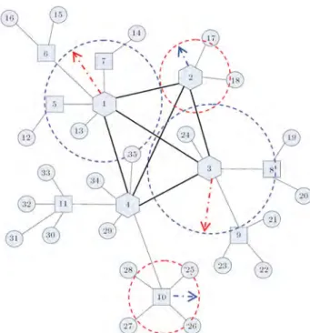
Figure 1 depicts a transportation network with two levels of hub facility and presents the problem with the best resolution. This network has 35 nodes. Non-hubs, hubs and central hubs are seen in the
Figure 1. A three level network on 35 nodes with 11 hubs and 4 central hubs.
shapes of circles, squares and hexagons, respectively. The covering radiuses of the hubs are traced with incomplete circles. There are various routes for the model depicted in Figure 1; for example, a route that visits 4 hubs in which trac demand ows from node 12 to node 21, and the ow paths including nodes 12 -5 - 1 - 3 - 9 - 21. One path, which encounters 2 hubs, crosses from node 17 to node 35 and its ow paths are 17 - 2 - 4 - 35. There are many trac paths in the problem, which can be observed in more detail in Figure 1.
This paper presents the hierarchical hub covering problem with dierent and xed covering radii for all hub facilities at all hierarchy levels. It aims to nd the location of hubs and central hubs, to allocate demand and hub nodes to the nearest located hub and central hub node in a unied covering situation, respectively. In addition, the paper guides the model for the better, seeking the solution area with predetermined radii. Radii are determined by an innovative method and they reduce CPU processing time. The main contributions of this paper are in proposing a new hub location problem and solving it in the best time by the heuristic identication of covering constraints. Computational results obtained for the CAB data, the Turkish network data and the Iranian Airport Data (IAD) on the proposed model show that this model is dierent from previous ones.
The rest of this paper is organized as follows: Section 2 presents a mixed integer programming for-mulation. Section 3 explains an innovative method for determining radii. Section 4 is dedicated to
computa-tional analysis, and investigating the performance of the model with the optimization solver, CPLEX 11.0, on the famous data sets of CAB, the Turkish network and IAD. The nal section develops the outcome of the paper.
2. A mixed integer programming formulation for SA-TH-HC
In this section, the notations, parameters and decision variables for our model are dened and then the mathematical formulation for the SA-TH-HC problem is presented. It is assumed that I is the set of nodes, H I is a potential hub set and C H is a set of possible locations for the central hubs. The parameters of the model include: PH, PC, H, ^H,
C, ^C, fij, Cij, tij, dij, rH, rC. As the model
has been designed for maximal covering, a constant number of hubs and central hubs must be established; we denote the number of hubs and central hubs by PH
and PC, respectively. In the hub location problems, a
discount rate of is applied to established link costs (or travel time) between hubs and 2 [0; 1]. The decreased coecients of routing cost and travel time among hubs and central hubs are presented with H,
^Hand those between central hubs are presented by C,
^C, respectively. It is assumed that these parameters
take values based on H C and ^H ^C [15].
Parameter fij is the amount of trac demand to be
routed from node i 2 I to node j 2 I, Cijis the routing
cost of unit ow demand between two nodes of i and j, tij is the travel time from node i to node j, and
dij is the distance between node i and node j. rH is
the amount of covering radius for all hubs and rC is
the amount of covering radius for all central hubs. As mentioned in previous studies, fii, Cii, tii and dii are
equal to zero for all of i 2 I. We symbolized the upper bound of the delivery time by , which is similar to the literature; is the maximum time by which any ow demand must reach its destination. The decision variables of the model are as follows:
Xijl 1 if node i is assigned to a hub at
node j and a central hub at node l; 0 otherwise.
Yi
jl The ow originated by node i 2 I (as
origin or destination) which crosses between the hub at node j and the central hub at node l.
Zi
kl The total demand ow which crosses
from the central hub at node k to the central hub at node l by node i 2 I as the origin or destination.
^
DI The time by which all the demand
ows from demand nodes and hubs assigned to central hub l arrive at l.
Si The time at which all the trac
originating at node i 2 I is available at node i (in a telecommunications context, letting Si= 0 for all i 2 I [15].
Consistent with the literature, if the variable Xjjl= 1 for each j 2 H, node j is assigned to a central
hub at node l, which means that node j is a hub node, and if Xlll = 1 for each l 2 C, node l is a central hub
node.
The objective function of our mathematical model minimizes the total routing costs of demand ow be-tween non-hubs and their hubs, bebe-tween the hubs and their central hubs and between central hubs together. According to the previously dened decision variables and parameters, the objective function is described in detail, as follows:
min z1=
X
i2I
X
r2I
(fir+ fri)
X j2H Cij X l2C xijl +X i2I X j2H X l2C:l6=j
HCjlyjli
+X i2I X k2C X l2C:l6=k
CCklzikl: (1)
The objective function could be investigated in three parts: (a), (b) and (c):
(a) P
i2I
P
r2I(fir+ fri)
P
j2HCij
P
l2Cxijl;
(b) P
i2I
P
j2H
P
l2C:l6=jHCjly i jl; (c) P i2I P k2C P
l2C:l6=kCCklz i kl.
According to part (a):
This formula calculates the routing cost of the es-tablished route between all demand nodes and their hub nodes, which is the result of forward ow (fir)
and return ow (fri) at each demand node with other
demand nodes. According to part (b):
This term calculates the total routing cost caused by the interaction of demand node i with other nodes, which passes the connecting rout of hub j and central hub l. In this case, the hub and the central hub must be dierent in order to form a route between them. According to part (c):
This term calculates the total routing cost caused by the interaction of demand node i with other nodes that
mathematical model for SA-TH-HC as follows: Single assignment hierarchical hub constraints:
X
j2H
X
l2C
xijl= 1 8i 2 I; (2)
xijl xjjl 8i 2 I; j 2 H : j 6= i; l 2 C; (3)
X
m2H
xjml xlll 8j 2 H; l 2 C : l 6= j; (4)
xljl= 0 8j 2 H; l 2 C : l 6= j; (5)
xijl2 f0; 1g 8i 2 I; j 2 H; l 2 C: (6)
Since the model was designed with the single assign-ment attribute, all non-hub nodes and hub nodes should be allocated to exactly one hub facility and one central hub facility, respectively. Constraints (2), (4) and (6) guarantee the single assignment attribute for the model. Constraints (4) ensure that each hub cannot be linked to other nodes unless that node is a central hub node. Constraints (3) state that if a demand node is assigned to another node, then, that node should be a hub node. Constraints (5) are unnecessary; however, they do make the LP relaxation stronger.
Number of hub and central hub constraints: X
j2H
X
l2C
xjjl= pH; (7)
X
l2C
xlll= pC: (8)
As the model was based on a P-hub median and maximal covering problems, we denoted the number of hubs and central hubs with Constraints (7) and (8), respectively:
Flow balance constraints: yi
jl
X
r2I:r6=j
(fir+ fri)(xijl xrjl) 8i 2 I;
j 2 H; l 2 C : l 6= j; (9) X k2C:k6=l zi lk X k2C:k6=l zi kl = X r2I fir X j2H
(xijl xrjl)
8i 2 I; l 2 C; (10)
yi
jl 0 8i 2 I; j 2 H; l 2 C; (11)
zi
The ow balance constraints are dened similar to Yaman's [15]. For each link, from a hub to its central hub, the amount of trac demand will be computed by Constraints (9) and (11). Through these constraints, the amount of trac crossing between a hub and its central hub is added as a lower bound for the yi
jl
variable; since the objective function is of a minimizing type, the least value of yi
jl is estimated. According to
ow network rules, the sum of input ow to a node is equal to the sum of output ow from the same node. This situation is ensured by ow balance Constraint (10) and Constraint (12), because the central hubs are end nodes of their hierarchy.
Covering constraints: X
j2H
X
l2C:j6=l
dijxijl rH 8i 2 I; (13)
X
l2C
dilxill rH 8i 2 I; (14)
djlxjjl rC 8j 2 H; l 2 C: (15)
We classied the solution space and modied the assignment procedure of each hub and non-hub node to the nearest facility at their top level. We specied that each assignment between two nodes occurs when they are in a specic closeness to each other. The specic closeness criteria are equal to the possible minimal distance between two node and they are characterized by rH and rC for second and rst level assignments,
respectively. We solved the model by investigating few local optimum solutions and, therefore, obtained the global optimum solution in the least possible time.
In short, all assignments were conducted by two xed amounts for rH and rC, which are computed by
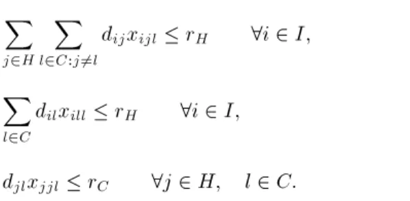
a a heuristic method and discussed in the next section. According to the above points, we designed Constraints (13), (14) and (15). Constraint (13) ensures that the assignment of demand nodes to hubs receives low services in a specic closeness criterion of rH. On
the other hand, the hierarchical model has a nested characteristic (in a nested hierarchy, a higher-level facility provides all the services provided by a lower level facility and at least one additional service; this is presented by Marianov and Serra [16]). So, it is possible that the non-hubs are assigned to a central hub to achieve low service. Then, Constraint (14) guarantees that assignment of demand nodes to central hubs receives low service in a specic closeness criterion of rH. Also, Constraint (15) guarantees that hub
nodes are assigned to central hubs and receive top service in a specic closeness criterion of rC. The
dierences between the current model and other models in literature stem from covering Constraints (13), (14)
and (15), which have the specic closeness criteria characterized by rH and rC for the second and rst
level assignments, respectively. Time bound constraints: ^
Dl
X
j2H
(Si+ tij+ ^Htjl)xijl 8i 2 I; l 2 C;
(16) Dl ^Dk+ ^Ctklxkkk 8l 2 C; k 2 C; (17)
Dl+
X
j2H
(^Htlj+ tji)xijl 8i 2 I; l 2 C;
(18) ^
Dl 0 8l 2 C: (19)
We dened the time bound constraints by using the ideas developed in Ernst et al. [11] and chiey Ya-man [15]. For the central hub of l, let ^Dl be the
time by which all the trac from demand nodes and hubs assigned to central hub l arrives at l. Constraint (16) guarantee that the time by which all the trac from demand nodes and hubs assigned to central hub l arrives at l is no earlier than the time the trac reaches from i to ^Dl. Constraint (17) calculates travel time
from each origin to the destination central hub and then the result is inserted into its ^Dl.
Constraint (18) ensures that the travel time of trac at each origin arrives at the destination at time or under. We presented a comprehensive output of the mathematical model with an example that is exhibited in Figures 2 and 3. The node set in Figure 2 is used as
Figure 2. The node set I.
Figure 4. The assignment state of m1 and m2nodes where trac of m2 is greater than the trac of m1.
Figure 5. The assignment state of m1and m2 nodes where trac of m1 is greater than trac of m2.
Figure 6. The assignment state of m1 and m2 nodes where trac of m2equals trac of m1.
an input model and the resulting network of the model is presented in Figure 3. According to this solution, x225 = x555 = x666 = x776 = x999 = x11119 = 1,
so, the nodes of 2, 5, 6, 7, 9 and 11 are chosen as hub nodes and also x555 = x666 = x999 = 1;
therefore, nodes of 5, 6, and 9 are selected as central hub nodes. The below notations are the time bound and covering constraints for the route between node 1 and node 8. The time bound constraints include (t12 + Ht25)x125 ^D5, ^D5+ Ct56x555 D6 and
D6+ (Ht67+ t78)x876 . The covering constraints
are d12x125 rH, d25x225 rC, d76x776 rC and
d87x876 rH. On the other hand, the notations of
ow balance Constraint (9) for nodes i = 1, j = 2 and l = 5 are (f12+f21)(x125 x225)+(f12+f21)x125+(f13+
f31)x125+(f14+f41)x125+ +(f112+f121)x125 y1251 .
Constraint (10) is another ow balance, so we selected the nodes of i = 1 and l = 5 as an example. The constraint is equal to (z1
56+ z951 ) (z165+ z195) = (f12+
f13+ f14+ + f112)x125 f12x255 f13x355 f15x555.
Also, this paper attempts to improve the hierarchical network structure which is investigated in Yaman [15]. Her output has some problems which lead to a one-way orientation, and create a special focus in one location. The present paper attempts to tackle the shortcomings of previous work using a transparent language, with perceived changes and a correct explanation of hier-archical structure. In addition to reduction in costs, which is investigated also in Yaman [15], we consider the balanced structure of the network, a reduction in the time of solution, an equal distribution of services, and promptness in providing services at all levels, by a change in the previous structure. Please consider the following logical reasoning;
Suppose points m1and m2as demand centers (or
third level), H1 and H2 as second level service centers
(or hub) and points C1 and C2 as rst level service
centers (or central hubs), which are shown by a circle, a triangle, and a square of the triangle, respectively. Also, fij is considered as trac, dijthe distance and tij
the travel time between two locations, i and j, which is dij = tij as the solution structure in Yaman [15] in the
literature, and, according to the above three conditions, 1, 2 and 3 are plotted.
In these gures, for a simpler description and preventing the expression of complex conditions, a particular state which will cover another scenario is studied, i.e. dc1C2; dH2C2 and dH1C1 are considered constant in all three states. Now consider Constraints (16) to (19) (i.e. time bound constraints). These constraints regard Figures 4, 5 and 6 as similar ones, because the time of providing services at all three states is equal, and they have the condition of being smaller than , unless exchange degrees, m1 and m2,
are dierent to other connections. In this case, three following states will occur, respectively:
1. If Pj2m2;H1;H2;C1;C2fm1j < P
j2m1;H1;H2;C1;C2 fm2j, without considering the fair distribution of services, the model chooses Figure 4 in order to reduce routing costs, because the total cost of the objective function is obtained by summation of distance multiplied by the trac.
2. If Pj2m2;H1;H2;C1;C2fm1j > P
j2m1;H1;H2;C1;C2 fm2j the model, as the above, chooses Figure 3 to reduce routing costs.
3. If Pj2m2;H1;H2;C1;C2fm1j = P
j2m1;H1;H2;C1;C2 fm2j the model will be apathetic in the choosing of gures, because routing costs in all three cases are the same.
As mentioned earlier, hierarchical problems, such as health and treatment or security forces, etc., have considered an equal distribution of services within the area of their goals and strategic values. Even the contemporary world provides various services in accordance with the fair distribution of services to draw attention and create a competitive advantage with other companies.
a major weakness in the third case, which state we have controlled by expressing covering Constraints (13)-(15). We are not allowed to exceed authorized and justiable limits, rH; rC, at the rst and second
servicing levels, and the demand nodes receive the service of dierent levels in a fair condition.
But, in cases 1 and 2, as mentioned in the computational results section, in return for an increase in Constraints (13)-(15), the total costs do not make many changes, and services are insignicant in return for creating fair distribution conditions.
According to the above, our model has considered the subject importance of fairness in providing services, which is signicantly important in the area of servicing; so that today, in addition to the general time limit (i.e. ) for providing various services, the time for providing primary care services or low level services (here, the second level ones) has a certain individual limit.
Figures 7 and 8 show feasible solutions with a structure of classication created by our allocation pattern for the second and rst service levels, respec-tively. A heuristic method for computing rH and rC is
introduced in the next section.
3. Proper parameters determination
A global optimal solution of the NP-complete problems is challenging in realistic sized cases. Similarly, for the problem discussed in this paper, it is dicult to determine a global solution. It can be seen that the problem is solved in a better time with the time
bound constraints. Also, there are other constraints in order to reach a global solution in the minimal amount of time. Hence, in this paper, we have provided an innovative method to determine the proper values of parameters rH and rC. So, we classify the total
solution space, and modify the assignment procedure of each non-hub node and each hub node to the next facilities at their top levels. We specify that each assignment occurs between two nodes when they are close to each other. The specic closeness criterion is equal to the least distance between two nodes. The specic closeness criteria are characterized by rH and
rC for second and rst level assignments, respectively.
So, in the process of solving the model, fewer solutions are surveyed and getting stuck at a local optimum solution is avoided. Therefore, the global solution is obtained more rapidly. We used a distance table to determine the radii. The columns of the distance table show the distances of a city to other cities. Initially, we obtained minimum distances in any column (without zero); they are the distance of cities close to each other. Also, we chose a maximum distance among the minimum distances of columns in the distance table for rH. This distance is the best value for the
covering radius of the second level, because if each distance is selected as being less, the model will be infeasible, and if a distance is selected further than that, the model will be farther from its ideal situation. Logically, the covering radiusof rst level is bigger than that of rH(rH rC), so, we will need a dominant
covering radius that is not very large, nor very small.
Figure 8. Pattern classication for the rst level of services.
Table 1. The heuristic method for determining the covering radiuses on distance table.
Row Descriptions
1 maxfminimum numbers into the columns (regardless of zero) of distance tableg = rH
2 minfmaximum numbers into columns of distance tableg = rC
Hence, we preferred a minimum distance among the maximum distances of columns in the distance table for rC. The maximum distances of columns denote
two cities the greatest distance from each other, and the minimum distance between them gives a dominant covering radius. However, we decreased and limited the space of the solution with a heuristic method. A procedure for determining radii is depicted in Table 1. We computed the rH and rC for the model. As a
result, we take rH = 695 and rC = 1506 for the
CAB data, rH = 377 and rC = 918 for the Turkish
network data, and rH = 479 and rC = 1390 for the
IAD data. The next section covers the computational analysis.
4. Computational Analysis
In the computational analysis, we applied the CAB data set, the Turkish network data set and the Iranian Aviation Dataset (IAD). The CAB data set is intro-duced by O'Kelly [2]. This data set contains ows and distances and is based on the airline passenger connections between 25 US cities in 1970 evaluated by the Civil Aeronautics Board (CAB) [1]. The global solutions are scaled through dividing by the total ow. We regarded all nodes as potential nodes for hubs and
central hubs, i.e. I = H = C, similar to the one used in Yaman [15], in order to compare it with our model. The Turkish network data set contains the data of distances, travel times, ows and xed link costs between 81 cities in Turkey and xed hub costs for these cities. The ow data is oered by Cetiner, Spil and Sural, and the xed link costs are suggested by Alumur, Kara and Karasan. The distances, travel times and xed hub costs are introduced by Tan and Kara and, nally, this data set is presented by Tan and Kara [12]. We applied Yaman's style in order to create a subset of the Turkish network data set, as we wanted to evaluate the eect of some parameters on the output of the model and investigate the procedure of computation times. To do this, we separated over 30 populated cities of the Turkish network data as the demand set I. There are the 21 populous cities in Turkey which belong to set I, from which we selected a set of 17 cities which had a cargo company. We chose them as a potential set of hubs (i.e., set of H) and determined a set of 10 cities with largest populations as a potential set of central hubs (i.e., set of C). Finally, we solved the model on all nodes in the Turkish network. The set of references were symbolized as I. We considered all 21 populous cities in Turkey as a potential set of hubs and located two central hubs in Ankara and Istanbul.
The IAD was presented by Karimi and Bashiri [17]. This data set includes the distances, costs, weights, capacities and xed charge hub costs based on the hub airport location between 37 Iranian cities. We regarded all the nodes as the demand set I, and we separated the 24 populous cities of IAD as a potential set of hubs (i.e., set of H) similar to Yaman [15] on the Turkish network data set. There are 16 populous cities in set H that have more than 100 units of capacity, so, we selected them as a potential set of central hubs (i.e., set of C). We presented the computational experience of the IAD data in Section 4.5.
4.1. Eect of changes in some parameters on the total cost
In the rst stage, we investigated the eects of time bound constraints and the number of central hubs on the routing costs. We solved the problem on the CAB data with n = 25 and PH = 5, and the Turkish network
data with n = 30 and PH = 7, where H= 0:9, C=
0:8, ^H = 0:9, ^C = f0:9; 0:8g and PC2 f1; ; PHg.
Similar to the application of each data set in Tan and Kara [12] (2007) and Yaman [15] (2009), we obtained the smallest for the problem, so that it becomes feasible when H = ^H = 0:9 and C = ^C = 0:8.
We calculated the average of the smallest amounts of for various values of PC. In order to have a strong
time bound, we presented amounts which are 120 and 240 times more than the average values. Therefore, we obtained 2 f2880; 3000; 1g for the CAB data and 2 f1740; 1860; 1g for the Turkish network data. For infeasible situations, we did not have any report. When great PC was enlarged, the results were presented for
both data sets, and the total cost had a decreasing trend in all cases. We assumed a basic state of cost with = rH = rC = 1 to see the procedure of total
cost with more clarication. Then, for each state, we computed the percent of increasing cost with the
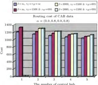
well-Figure 9. A chart of total routing cost for the CBA data with n = 25, PH= 5 and ^C= 0:8.
known formula of:
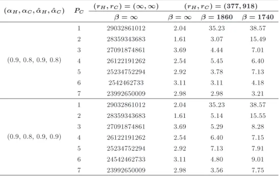
%increasing cost = New cost Basic costBasic cost 100: The computation is presented in Table 2 and Figure 9 for the CAB data and Table 3 and Figure 10 for the Turkish network data.
For the CAB data, the total cost is increased on average by 6:27% for both ^C = 0:8 and ^C = 0:9,
while covering radii are imposed on the model. The problem is infeasible while PC = 1 and imposes time
bound constraints on the model. Also, it is infeasible with two central hubs, while = 2880 and ^C = 0:9.
In most cases, when PC = 2, the problem becomes
feasible with the time bound constraints; however the total routing cost increases by 13.29% when it has a feasible solution. As revealed in Table 2, by decrease in value of , the problem needs more central hubs to become a feasible solution. Generally, the total cost increases by the covering and the time bound
Table 2. Total routing cost and cost increasing percent for the CAB data with n = 25, PH= 5 and = f2880; 3000; 1g.
(H; C; ^H; ^C) PC (rH; rC) = (1; 1) (rH; rC) = (695; 1506)
= 1 = 1 = 3000 = 2880
(0.9, 0.8, 0.9, 0.8)
1 1200.13 10.67 -
-2 1146.79 6.04 13.29 13.29
3 1108.35 5.23 9.92 9.92
4 1065.06 5.54 7.53 8.58
5 1034.10 3.87 4.73 8.69
(0.9, 0.8, 0.9, 0.9)
1 1200.13 10.67 -
-2 1146.79 6.04 13.29
-3 1108.35 5.23 9.92 9.92
4 1065.06 5.54 8.58 11.33
(H; C; ^H; ^C) PC
= 1 = 1 = 1860 = 1740
(0.9, 0.8, 0.9, 0.8)
1 29032861012 2.04 35.23 38.57
2 28359343683 1.61 3.07 15.49
3 27091874861 3.69 4.44 7.01
4 26122191262 2.54 5.45 6.40
5 25234752294 2.92 3.78 7.13
6 2542462733 3.11 3.11 4.18
7 23992650009 2.98 2.98 3.21
(0.9, 0.8, 0.9, 0.9)
1 29032861012 2.04 35.23 38.57
2 28359343683 1.61 5.14 15.55
3 27091874861 3.69 5.29 8.28
4 26122191262 2.54 6.40 7.15
5 25234752294 2.92 7.13 7.91
6 24542462733 3.11 4.80 9.01
7 23992650009 2.98 3.56 7.75
Figure 10. A chart of total routing cost for the Turkish data with n = 30, PH= 7 and ^C= 0:8.
constraints, and the increased percentage of the total cost is equal to, on average, 3.69%, when ^C = 0:8,
and 4.95% when ^C = 0:9 from = 1 to = 2880.
But, Figure 9 shows the growth rate of the total cost which is very negligible compared to the equal covering situation.
For the Turkish network data, the problem is feasible for all cases. Whenever the time bound constraint is imposed on the problem, the total cost increases on average by 5.59% when ^C = 0:8 and
6.95% when ^C = 0:9 from = 1 to = 1860. The
growth rate of the total cost increases with imposing the , when PC is equal to 1. Table 2 shows that
while covering radii are imposed on the problem, the total cost increases, on average, 2.70% for all instances. Figure 10 displays the increasing procedure of the total
cost, but this growth rate is very negligible compared to the equal covering situation.
Finally, we infer that, by imposing the covering radii and delivering the time bound, the total cost increases in both data sets. The distances between hubs and central hubs are in the range of rC, and the range of
distances among non-hubs and hubs is rH by covering
constraints. So, if two demand nodes and their hubs are assigned to dierent hubs and central hubs, the distances between origin-destination pairs include two rH and one rC. If the output of the model moves from
a complete network to a star network by decreasing central hubs, the rC does not come to the distances
between each origin-destination pair.
4.2. Eect of change in some parameters on the locations of central hub
In this subsection, we report the locations of central hubs and hubs in the optimum solutions for the CAB data with n = 25, PH = 5, PC = 2, 3, 4, the Turkish
network data with n = 30, PH = 7, PC = 3, 4, 5 and
in both of them with dierent amounts of time bound (i.e., ), covering radii (i.e., rH and rC) and discount
coecients (i.e. H, C, ^H and ^C).
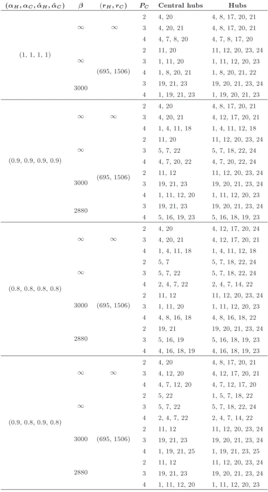
These reports are presented in Tables 4 and 5 for CAB data and Turkish network data, respectively. Table 4 shows that when = 1 and (rH; rC) = 1
cities 4 and 20 are selected as central hubs in 100% and 87% of cases, respectively. But when = 1 and (rH; rc) = (695; 1506), these percentages are decreased
by 27% and 34%. Cities 11 and 12 are selected as central hubs in all instances with PC= 2, = 3000 and
Table 4. The locations of central hubs and hubs for the CAB data. (H; C; ^H; ^C) (rH; rC) PC Central hubs Hubs
(1, 1, 1, 1)
1 1
2 4, 20 4, 8, 17, 20, 21 3 4, 20, 21 4, 8, 17, 20, 21 4 4, 7, 8, 20 4, 7, 8, 17, 20 1
(695, 1506)
2 11, 20 11, 12, 20, 23, 24 3 1, 11, 20 1, 11, 12, 20, 23 4 1, 8, 20, 21 1, 8, 20, 21, 22 3000 3 19, 21, 23 19, 20, 21, 23, 24
4 1, 19, 21, 23 1, 19, 20, 21, 23
(0.9, 0.9, 0.9, 0.9)
1 1
2 4, 20 4, 8, 17, 20, 21 3 4, 20, 21 4, 12, 17, 20, 21 4 1, 4, 11, 18 1, 4, 11, 12, 18 1
(695, 1506)
2 11, 20 11, 12, 20, 23, 24 3 5, 7, 22 5, 7, 18, 22, 24 4 4, 7, 20, 22 4, 7, 20, 22, 24 3000
2 11, 12 11, 12, 20, 23, 24 3 19, 21, 23 19, 20, 21, 23, 24 4 1, 11, 12, 20 1, 11, 12, 20, 23 2880 3 19, 21, 23 19, 20, 21, 23, 24
4 5, 16, 19, 23 5, 16, 18, 19, 23
(0.8, 0.8, 0.8, 0.8)
1 1
2 4, 20 4, 12, 17, 20, 24 3 4, 20, 21 4, 12, 17, 20, 21 4 1, 4, 11, 18 1, 4, 11, 12, 18 1
(695, 1506)
2 5, 7 5, 7, 18, 22, 24 3 5, 7, 22 5, 7, 18, 22, 24 4 2, 4, 7, 22 2, 4, 7, 14, 22 3000
2 11, 12 11, 12, 20, 23, 24 3 1, 11, 20 1, 11, 12, 20, 23 4 4, 8, 16, 18 4, 8, 16, 18, 22 2880
2 19, 21 19, 20, 21, 23, 24 3 5, 16, 19 5, 16, 18, 19, 23 4 4, 16, 18, 19 4, 16, 18, 19, 23
(0.9, 0.8, 0.9, 0.8)
1 1
2 4, 20 4, 8, 17, 20, 21 3 4, 12, 20 4, 12, 17, 20, 21 4 4, 7, 12, 20 4, 7, 12, 17, 20 1
(695, 1506)
2 5, 22 1, 5, 7, 18, 22 3 5, 7, 22 5, 7, 18, 22, 24 4 2, 4, 7, 22 2, 4, 7, 14, 22 3000
2 11, 12 11, 12, 20, 23, 24 3 19, 21, 23 19, 20, 21, 23, 24 4 1, 19, 21, 25 1, 19, 21, 23, 25 2880
2 11, 12 11, 12, 20, 23, 24 3 19, 21, 23 19, 20, 21, 23, 24 4 1, 11, 12, 20 1, 11, 12, 20, 23
(0.9, 0.8, 0.9, 0.9)
1 1
2 4, 20 4, 8, 17, 20, 21 3 4, 12, 20 4, 12, 17, 20, 21 4 4, 7, 12, 20 4, 7, 12, 17, 20 1
(695, 1506)
2 5, 22 1, 5, 7, 18, 22 3 5, 7, 22 5, 7, 18, 22, 24 4 2, 4, 7, 22 2, 4, 7, 14, 22
3000 2 11, 12 11, 12, 20, 23, 24
3 19, 21, 23 19, 20, 21, 23, 24 4 1, 11, 12, 20 1, 11, 12, 20, 23 2880 3 19, 21, 23 19, 20, 21, 23, 24
4 5, 16, 19, 23 5, 16, 18, 19, 23
hubs in 100% and 87% of cases, respectively. But, when = 1 and (rH; rC) = (695; 1506). We observed
that when the time bound does not exist, PC= 3 and
(rH; rC) = (695; 1506), cities 5, 7 and 22 are selected as
central hubs. The cities 19, 21 and 23 appear as central hubs in more instances when the time bound and the covering constraints are applied to the problem and when PC= 3. Generally, the covering constraints cause
many changes in the locations of central hubs and the change in parameters cannot set the exact procedure. We observed that by imposing covering constraints and simultaneously decreasing the procedure of values of discount coecients, the locations of central hubs in the optimum solutions are signicantly aected. For example, when = 1, and PC = 3, cities 4, 20, and
21 are central hubs in a situation where all discount coecients are 1 and (rH; rC) = 1, and cities 5, 7, and
22 are central hubs in a situation where all discount coecients are 0.8 and (rH; rC) = (695; 1506). Not
only do all central hubs transfer from one place to another, but also they are located far from cities 4, 20 and 21.
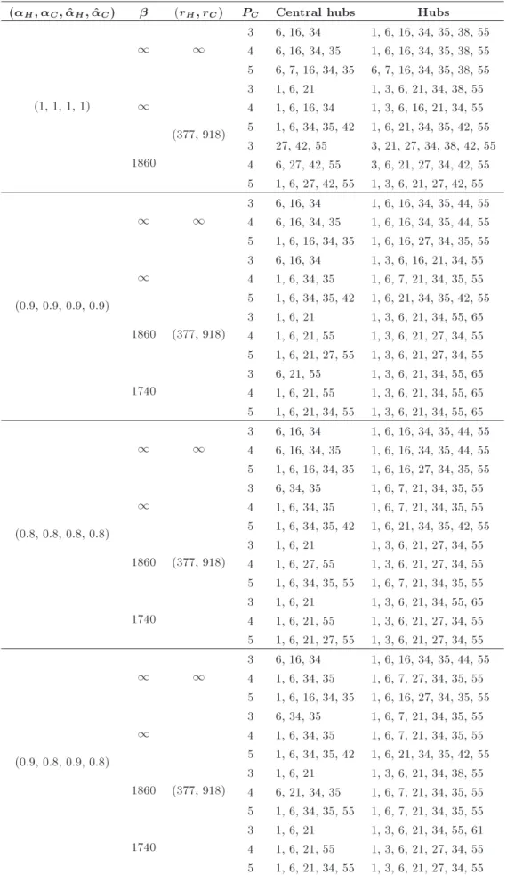
Table 5 shows that when C = H, = 1 and
(rH; rC) = 1, cities 6, 16 and 34 are chosen as central
hubs in all cases, but these cities will be changed to cities 6, 34 and 35 in a situation when the covering constraints are considered in the problem. Also, city 55 is selected as the central hub in most cases where there exist a time bound and covering constraints. City 6 is chosen as the central hub in all situations except the state of PC = 3, = 1860 and C = H = 1. A
memorable city is city 55 because it appears as a hub in all instances. Generally, we observed that imposing the time bound and covering constraints and further restricting the space of the solution with decreasing lead to some changes in cities and a transfer of central hub locations to other cities.
Figure 11 shows the frequency percentage of se-lecting each potential city as a central hub. Considering
Figure 11. Frequency diagram of potential 10 cities of central hubs for Turkish data.
this diagram, cities 6, 1 and 34 have been selected as central hubs in most items over total runs. Besides, city 7 appears as a top level facility in 2% of total instances. Also, in this data set, we noticed that covering restrictions are eective on locations of the top level facilities. For example, when = 1, PC = 3 and
H = C = 1, cities 6, 16 and 34 have been selected
as central hubs for (rH; rC) = 1, but the cities of 1, 6
and 21 have been selected as central hubs for (rH; rC) =
(377; 918), so, two facilities of three central hubs have been transferred. Cities 6 and 21 are selected as top level facilities in all instances by = 1740. This shows that when the time bound restrictions are strict, these cities have the best covering. Imposing, simultaneously, the time bound and covering constraints, leads to convergence of the locations of central hubs.
4.3. Eect of change in some parameters on computational time
In this subsection, we studied the eect of the param-eters of the problem on computation times. We solved our model using GAMS 21.7 and CPLEX 11.0.0 on a personal computer with a 2.10GHz Intel Core 2 Duo processor and 3GB of RAM operating under the system Windows 7 Ultimate.
Table 5. The locations of central hubs and hubs for the Turkish netword data. (H; C; ^H; ^C) (rH; rC) PC Central hubs Hubs
(1, 1, 1, 1)
1 1
3 6, 16, 34 1, 6, 16, 34, 35, 38, 55 4 6, 16, 34, 35 1, 6, 16, 34, 35, 38, 55 5 6, 7, 16, 34, 35 6, 7, 16, 34, 35, 38, 55 1
(377, 918)
3 1, 6, 21 1, 3, 6, 21, 34, 38, 55 4 1, 6, 16, 34 1, 3, 6, 16, 21, 34, 55 5 1, 6, 34, 35, 42 1, 6, 21, 34, 35, 42, 55 1860
3 27, 42, 55 3, 21, 27, 34, 38, 42, 55 4 6, 27, 42, 55 3, 6, 21, 27, 34, 42, 55 5 1, 6, 27, 42, 55 1, 3, 6, 21, 27, 42, 55
(0.9, 0.9, 0.9, 0.9)
1 1
3 6, 16, 34 1, 6, 16, 34, 35, 44, 55 4 6, 16, 34, 35 1, 6, 16, 34, 35, 44, 55 5 1, 6, 16, 34, 35 1, 6, 16, 27, 34, 35, 55 1
(377, 918)
3 6, 16, 34 1, 3, 6, 16, 21, 34, 55 4 1, 6, 34, 35 1, 6, 7, 21, 34, 35, 55 5 1, 6, 34, 35, 42 1, 6, 21, 34, 35, 42, 55 1860
3 1, 6, 21 1, 3, 6, 21, 34, 55, 65 4 1, 6, 21, 55 1, 3, 6, 21, 27, 34, 55 5 1, 6, 21, 27, 55 1, 3, 6, 21, 27, 34, 55 1740
3 6, 21, 55 1, 3, 6, 21, 34, 55, 65 4 1, 6, 21, 55 1, 3, 6, 21, 34, 55, 65 5 1, 6, 21, 34, 55 1, 3, 6, 21, 34, 55, 65
(0.8, 0.8, 0.8, 0.8)
1 1
3 6, 16, 34 1, 6, 16, 34, 35, 44, 55 4 6, 16, 34, 35 1, 6, 16, 34, 35, 44, 55 5 1, 6, 16, 34, 35 1, 6, 16, 27, 34, 35, 55 1
(377, 918)
3 6, 34, 35 1, 6, 7, 21, 34, 35, 55 4 1, 6, 34, 35 1, 6, 7, 21, 34, 35, 55 5 1, 6, 34, 35, 42 1, 6, 21, 34, 35, 42, 55 1860
3 1, 6, 21 1, 3, 6, 21, 27, 34, 55 4 1, 6, 27, 55 1, 3, 6, 21, 27, 34, 55 5 1, 6, 34, 35, 55 1, 6, 7, 21, 34, 35, 55 1740
3 1, 6, 21 1, 3, 6, 21, 34, 55, 65 4 1, 6, 21, 55 1, 3, 6, 21, 27, 34, 55 5 1, 6, 21, 27, 55 1, 3, 6, 21, 27, 34, 55
(0.9, 0.8, 0.9, 0.8)
1 1
3 6, 16, 34 1, 6, 16, 34, 35, 44, 55 4 1, 6, 34, 35 1, 6, 7, 27, 34, 35, 55 5 1, 6, 16, 34, 35 1, 6, 16, 27, 34, 35, 55 1
(377, 918)
3 6, 34, 35 1, 6, 7, 21, 34, 35, 55 4 1, 6, 34, 35 1, 6, 7, 21, 34, 35, 55 5 1, 6, 34, 35, 42 1, 6, 21, 34, 35, 42, 55 1860
3 1, 6, 21 1, 3, 6, 21, 34, 38, 55 4 6, 21, 34, 35 1, 6, 7, 21, 34, 35, 55 5 1, 6, 34, 35, 55 1, 6, 7, 21, 34, 35, 55 1740
3 1, 6, 21 1, 3, 6, 21, 34, 55, 61 4 1, 6, 21, 55 1, 3, 6, 21, 27, 34, 55 5 1, 6, 21, 34, 55 1, 3, 6, 21, 27, 34, 55
(0.9, 0.8, 0.9, 0.9)
1 1 4 1, 6, 34, 35 1, 6, 7, 27, 34, 35, 55 5 1, 6, 16, 34, 35 1, 6, 16, 27, 34, 35, 55 1
(377, 918)
3 6, 34, 35 1, 6, 7, 21, 34, 35, 55 4 1, 6, 34, 35 1, 6, 7, 21, 34, 35, 55 5 1, 6, 34, 35, 42 1, 6, 21, 34, 35, 42, 55 1860
3 1, 6, 21 1, 3, 6, 21, 34, 55, 65 4 1, 6, 21, 55 1, 3, 6, 21, 27, 34, 55 5 1, 6, 21, 34, 55 1, 3, 6, 21, 27, 34, 55 1740
3 6, 21, 55 1, 3, 6, 21, 34, 55, 65 4 1, 6, 21, 55 1, 3, 6, 21, 34, 55, 65 5 1, 6, 21, 34, 55 1, 3, 6, 21, 34, 55, 65 Table 6. The CPU time for CAB data with n = 25 and PH= 5:
(H; C; ^H; ^C) PC (rH; rC) = (1; 1) (rH; rC) = (695; 1506)
= 1 = 1 = 3000 = 2880
(1, 1, 1, 1)
1 477.38 17.52 -
-2 19355.87 571.99 -
-3 12755.77 3005.96 158.50
-4 26657.54 2639.64 1141.48
-5 288.00 33.55 29.98
-(0.9, 0.9, 0.9, 0.9)
1 685.46 18.85 -
-2 35826.54 868.42 254.59
-3 20098.73 2282.89 755.45 320.16
4 70216.72 3788.04 1293.89 794.01
5 253.02 90.86 19.83 17.52
(0.8, 0.8, 0.8, 0.8)
1 1642.01 21.50 -
-2 12126.83 698.31 3306.31 1568.32
3 17357.99 2365.05 3301.53 4696.96
4 34253.30 2950.95 4426.40 2360.16
5 150.06 25.50 44.47 35.28
(0.9, 0.8, 0.9, 0.8)
1 635.74 16.11 -
-2 61561.77 621.98 1845.51 32.64
3 51699.33 3026.62 3665.95 505.02
4 19831.40 3022.81 2627.58 373.06
5 141.30 24.42 46.18 21.25
(0.9, 0.8, 0.9, 0.9)
1 635.74 13.56 -
-2 61561.77 610.42 204.13
-3 51699.33 2812.99 618.65 247.27
4 19831.40 2286.67 488.73 1005.40
5 141.30 26.46 29.69 15.07
for infeasible cases. The computational study for CAB data was performed with n = 25, PH = 5,
= f2880; 3000; 1g and dierent values of PC and
discount coecients. The results for the CAB data are depicted in Table 6 and Figure 10. We reported the computational times in Yaman [15] for the basic state of CAB data (i.e., = 1 and (rH; rC) = 1) in
the rst column of the left side (Table 6), in order for readers to observe the dierences between the proposed model with that of previous studies. Table 6 shows that the dierent cases of the problem are solved, on average, 91.62% faster using covering constraints rather than non-covering ones, while the computational times of the problem are increased in all cases, except when
PC = 4 and = 3000. All cases with PH = PC are the
easiest.
Whereas the covering restrictions improve CPU times in all cases, imposing the time bound constraints do not improve the computation times; for example, when = 3000 and all reduction factors are 0.8 for all PC, the computational times get worse in all instances.
When = 3000, H = 0:9 and C= 0:8, the CPU time
is improved only for PC= 4, but it increases for other
PC. Also, the CPU times increase in H = C = 0:8
with PC= 2 and 3 when the upper bound for the time
bound is equal to 2880. The computational study for the Turkish network data was performed with n = 30, PH = 7, = f1740; 1860; 1g and dierent values of
PC and discount coecients. The results are depicted
in Table 7 and Figure 12. Table 7 shows that all the problems are solved, on average, 86.17% faster
Figure 12. A chart of procedure of CPU time for the Turkish network data with n = 30 and PH= 7.
Table 7. The CPU time for Turkish network data with n = 30, PH= 7.
(H; C; ^H; ^C) PC (rH = 1; rC) = 1 = 1(rH; r = 1860C) = (377; 918) = 1740
(1, 1, 1, 1)
1 317.53 5.15 -
-2 4044.978 23.60 6.41
-3 1593.769 47.67 13.33
-4 1129.881 62.36 16.73
-5 903.86 47.37 21.85
-6 518.87 34.92 13.79
-7 11.23 3.42 2.36
-(0.9, 0.9, 0.9, 0.9)
1 175.51 4.53 4.54 4.78
2 2214.94 35.29 12.49 6.75
3 837.67 37.29 19.38 14.22
4 700.64 43.39 26.34 16.16
5 603.36 28.09 72.89 18.11
6 325.08 35.25 23.21 13.88
7 4.89 2.82 2.47 2.30
(0.8, 0.8, 0.8, 0.8)
1 165.52 3.39 5.46 6.07
2 2520.53 36.75 15.83 27.55
3 4128.00 46.04 42.94 66.57
4 775.40 33.22 108.21 75.64
5 447.10 18.80 24.24 124.43
6 304.29 21.21 15.22 21.42
7 4.06 3.16 2.66 2.47
(0.9, 0.8, 0.9, 0.8)
1 332.61 5.09 5.19 4.35
2 1209.82 17.11 13.90 16.12
3 914.50 30.82 25.76 60.48
4 579.29 17.24 53.87 63.56
5 559.03 21.10 26.77 73.09
6 103.33 19.69 15.28 51.77
7 5.57 2.42 2.60 2.22
(0.9, 0.8, 0.9, 0.9)
1 282.34 4.54 4.80 4.71
2 1356.15 18.77 10.30 6.70
3 936.87 35.58 22.88 14.38
4 553.84 22.43 48.24 19.37
5 360.47 24.48 43.27 18.13
6 26.13 22.59 18.86 14.95
cases with PH = PC are the easiest. In this data
set, when the time bound constraints are imposed on the model, CPU time gets worse in some cases. For example, when = 1860, the computational times get worse in all instances (except when all reduction factors are 1) for PC= 5. Also, when = 1740, the CPU times
increase in PC= 3, 4, 5 and 6 for H = C = 0:8 and
H= 0:9, C= 0:8.
CPU times are depicted in Figures 12 and 13 for Turkish network data and CAB data, respectively. The gures indicate that computational times have signicantly decreased by our heuristic method, which is indicative of an excellent improvement. These improvements are so eective that they overshadow the
Figure 13. A chart of procedure of CPU time for the CAB data with n = 25 and PH= 5.
Figure 14. The map for Turkish network data with n = 30, 17 and 10 number of potential nodes for hubs and central hubs, respectively. Adapted from Yaman
(2009) [15].
poor increasing procedure of costs depicted in Figures 9 and 10. Figure 14 shows 30 selected nodes on the map of Turkey. The potential nodes of central hubs and hubs are characterized by squares and circles, respectively.
4.4. The problem with two central hubs located in Ankara and Istanbul
We solved the problem with all nodes in the Turkish network data. We set PC = 2 and located that in
Ankara and Istanbul.
We computed rC by the heuristic method, where
rC = 1046, but set rH = 477, whose amount is
100 units higher than rH for the set of 30 nodes, so,
the problem needs fewer hubs for maximal covering. We took H = ^H = 0:9, C = ^C = 0:8, =
f2640; 2700; 1g and PH = 7 similar to the work done
by Yaman [15], as we wanted to have readers compare it with our work. These results are depicted in Table 8. We observed that the results are equal for each PH
Table 8. The results for Turkish network with n = 81, rC= 1046, rH= 477 and two central hubs in Ankara and Istanbul.
PH Cost Hubs CPU time
1
7 62778796527.80 1, 3, 6, 21, 25, 34, 55 7.293 8 62306026267.80 1, 3, 6, 21, 25, 34, 44, 55 15.282 9 62135009710.80 1, 3, 6, 16, 21, 25, 34, 44, 55 19.904 10 62005078818.20 1, 3, 6, 16, 21, 25, 34, 42, 44, 55 22.483 11 61881337592.50 1, 3, 6, 21, 25, 26, 34, 42, 44, 55, 81 16.069 12 61777489330.20 1, 3, 6, 21, 25, 26, 34, 38, 42, 44, 55, 81 12.117
2700
7 62778796527.80 1, 3, 6, 21, 25, 34, 55 10.072 8 62306026267.80 1, 3, 6, 21, 25, 34, 44, 55 18.781 9 62135009710.80 1, 3, 6, 16, 21, 25, 34, 44, 55 25.905 10 62005078818.20 1, 3, 6, 16, 21, 25, 34, 42, 44, 55 12.176 11 61881337592.50 1, 3, 6, 21, 25, 26, 34, 42, 44, 55, 81 13.257 12 61777489330.20 1, 3, 6, 21, 25, 26, 34, 38, 42, 44, 55, 81 12.978
2640
7 62778796527.80 1, 3, 6, 21, 25, 34, 55 9.890 8 62306026267.80 1, 3, 6, 21, 25, 34, 44, 55 16.622 9 62135009710.80 1, 3, 6, 16, 21, 25, 34, 44, 55 23.275 10 62005078818.20 1, 3, 6, 16, 21, 25, 34, 42, 44, 55 17.181 11 61881337592.50 1, 3, 6, 21, 25, 26, 34, 42, 44, 55, 81 16.188 12 61777489330.20 1, 3, 6, 21, 25, 26, 34, 38, 42, 44, 55, 81 6.960
in dierent amounts of . Table 8 shows that results have been converged by the covering radii. All CPU times occur within 26 seconds in all instances, which it is a very good result in the large scale problem. We solved the problem without covering restrictions for PH = 7, whose CPU time amounted to 1609.409
seconds, total cost to 62103232960.50 and locations of hubs to 1, 3, 6, 25, 34, 44 and 55. First, we presented a map of 81 cities and the potential node sets for hubs and central hubs in Figure 15. Then, this result comes in Figure 16 for making a simpler comparison with the results by covering restrictions in Figure 17. It should be noted that hubs have been specied by black squares. Figures 16 and 17 indicate that the problem is solved in the best time and hubs are eectively dispersed by covering constraints. 4.5. Computational research on the IAD data We solved the problem on the IAD data with n = 37 and PH = 9, and examined the eect of time bound
Figure 15. The map for Turkish network data with n = 81 and 21 number of potential nodes for hubs and two central hubs located in Ankara and Istanbul. Adapted from Yaman (2009) [15].
Figure 16. The hub network for n = 81, C= 0:8,
H= 0:9, PH = 7 and = 1.
Figure 17. The hub network for n = 81, C= 0:8,
H= 0:9, PH = 7 and = 1, 2700, 2640.
constraints, the number of central hubs and covering constraints for various values of decreasing coecients on the routing costs.
We dened the problem on the IAD data with n = 37 and PH = 9, where H, C, ^H, ^C =
f0:9; 0:8g and PC 2 f1; ; PHg. Similar to the
work by Tan and Kara (2007) and Yaman (2009), we calculated the amounts of . Therefore, we dened 2 f2880; 3000; 1g for the IAD data. For an infeasible situation, we do not have any report. We reported locations of central hubs and hubs in the optimum solutions with n = 37, PH = 9, PC = 1; 2; 3 and 4
with dierent types of time bound (i.e., ), covering radii (i.e., rH and rC) and H = C = ^H = ^C =
f0:8; 0:9g (see Table 9).
Cities 10 and 31 are chosen as central hubs in 92% of cases, but city 31 has been changed to city 36 in 4 instances, when PC = 2 and the covering constraints
are considered in the problem. For example, when PC = 2, (rH; rC) = (479; 1390), = 3000 and
(H; C; ^H; ^C) = (0:9; 0:8; 0:9; 0:8). Also cities 2,
5, 10, 31 and 34 are selected as hub nodes for 100% of cases with the time bound and covering constraints and without them. City 19 is chosen as the hub node in all instances except when PC = 1, = 1, rH = rC = 1
and H = ^H = 0:9. Memorable cities are 10 and 31 in
Table 9, since they appear as central hub and hub nodes in more than 92% and 100% of instances, respectively. In general, we see that imposing the time bound and covering constraints and further restricting the space of solution with decreasing lead to changes in cities and transfer of central hub locations to other cities. The computational times for infeasible cases have not been reported. The computational study for IAD data is conducted by n = 37, PH = 9, = f2880; 3000; 1g
and dierent values of PC and discount coecients.
The CPU time for IAD data are reported in Table 10. Figure 18 shows that, in dierent cases, the problem
Figure 18. A chart of procedure of CPU time for the IAD data with n = 37, PH= 9 and = (0:8; 0:8; 0:8; 0:8).
(0.9, 0.9, 0.9, 0.9)
1 1
1 10 2, 5, 8, 10, 18, 26, 28, 31, 34 2 10, 31 2, 5, 10, 16, 19, 30, 31, 34, 36 3 10, 19, 31 2, 5, 10, 16, 19, 25, 30, 31, 34 4 10, 16, 19, 31 2, 5, 10, 16, 19, 25, 30, 31, 34
1
(479, 1390)
1 10 2, 4, 5, 10, 19, 24, 31, 34, 36 2 10, 31 2, 5, 10, 16, 19, 30, 31, 34, 36 3 10, 19, 31 2, 5, 10, 16, 19, 30, 31, 34, 36 4 10, 19, 31, 36 2, 5, 10, 16, 19, 30, 31, 34, 36
3000
1 28 2, 5, 19, 22, 24, 28, 31, 34, 36 2 10, 36 2, 4, 5, 10, 19, 24, 31, 34, 36 3 10, 19, 31 2, 5, 10, 16, 19, 30, 31, 34, 36 4 10, 19, 31, 36 2, 5, 10, 16, 19, 30, 31, 34, 36
2880
1
-2 10, 36 2, 4, 5, 10, 19, 24, 31, 34, 36 3 10, 31, 36 2, 5, 10, 16, 19, 30, 31, 34, 36 4 10, 19, 31, 36 2, 5, 10, 16, 19, 30, 31, 34, 36
(0.8, 0.8, 0.8, 0.8)
1 1
1 10 2, 5, 10, 15, 18, 19, 28, 31, 34 2 10, 31 2, 5, 10, 16, 19, 28, 30, 31, 34 3 10, 19, 31 2, 5, 10, 16, 19, 28, 30, 31, 34 4 10, 16, 19, 31 2, 5, 10, 16, 19, 28, 30, 31, 34
1
(479, 1390)
1 10 2, 4, 5, 10, 19, 24, 31, 34, 36 2 10, 31 2, 5, 10, 16, 19, 30, 31, 34, 36 3 10, 19, 31 2, 5, 10, 16, 19, 30, 31, 34, 36 4 10, 19, 31, 36 2, 5, 10, 16, 19, 30, 31, 34, 36
3000
1 10 2, 4, 5, 10, 19, 24, 31, 34, 36 2 10, 31 2, 5, 10, 16, 19, 30, 31, 34, 36 3 10, 19, 31 2, 5, 10, 16, 19, 30, 31, 34, 36 4 10, 19, 31, 36 2, 5, 10, 16, 19, 30, 31, 34, 36
2880
1 10 2, 4, 5, 10, 19, 24, 31, 34, 36 2 10, 31 2, 5, 10, 16, 19, 30, 31, 34, 36 3 10, 19, 31 2, 5, 10, 16, 19, 30, 31, 34, 36 4 10, 19, 31, 36 2, 5, 10, 16, 19, 30, 31, 34, 36
(0.9, 0.8, 0.9, 0.8)
1 1
1 10 2, 5, 8, 10, 18, 26, 28, 31, 34 2 10, 31 2, 5, 10, 16, 19, 25, 30, 31, 34 3 10, 19, 31 2, 5, 10, 16, 19, 25, 30, 31, 34 4 10, 16, 19, 31 2, 5, 10, 16, 19, 25, 30, 31, 34
1
(479, 1390)
1 10 2, 4, 5, 10, 19, 24, 31, 34, 36 2 10, 31 2, 5, 10, 16, 19, 30, 31, 34, 36 3 10, 19, 31 2, 5, 10, 16, 19, 30, 31, 34, 36 4 10, 19, 31, 36 2, 5, 10, 16, 19, 30, 31, 34, 36
3000
1 28 2, 5, 19, 22, 24, 28, 31, 34, 36 2 10, 36 2, 4, 5, 10, 19, 24, 31, 34, 36 3 10, 19, 31 2, 5, 10, 16, 19, 30, 31, 34, 36 4 10, 19, 31, 36 2, 5, 10, 16, 19, 30, 31, 34, 36
2880
-
-2 10, 36 2, 4, 5, 10, 19, 24, 31, 34, 36 3 10, 19, 31 2, 5, 10, 16, 19, 30, 31, 34, 36 4 10, 19, 31, 36 2, 5, 10, 16, 19, 30, 31, 34, 36
Table 10. The CPU time for IAD data with n = 37 and PH= 9.
(H; C; ^H; ^C) PC (rH; rC) = 1 (rH; rC) = (479; 1390)
= 1 = 1 = 3000 = 2880
(0.9, 0.9, 0.9, 0.9)
1 1691.04 9.59 22.15
-2 2358.87 29.30 37.55 28.17
3 1139.30 34.99 51.13 134.20
4 1215.54 41.27 31.49 29.42
(0.8, 0.8, 0.8, 0.8)
1 1323.30 8.49 15.10 11.99
2 1070.69 34.95 26.64 35.93
3 1066.78 33.30 37.68 58.31
4 1001.85 29.71 31.38 36.53
(0.9, 0.8, 0.9, 0.8)
1 1244.33 9.85 22.25
-2 1644.72 23.80 58.27 40.71
3 1373.03 21.60 73.73 51.04
4 1084.30 31.47 29.11 27.77
Figure 19. The map for IAD data with n = 37, 24 and 16 number of potential nodes for hubs and central hubs, respectively. Adapted from Karimi (2011).
is solved, on average, 97% faster (i.e., the CPU time decreases more than 97%) with covering constraints rather than with non-covering ones, so it is similar to Tables 6 and 7).
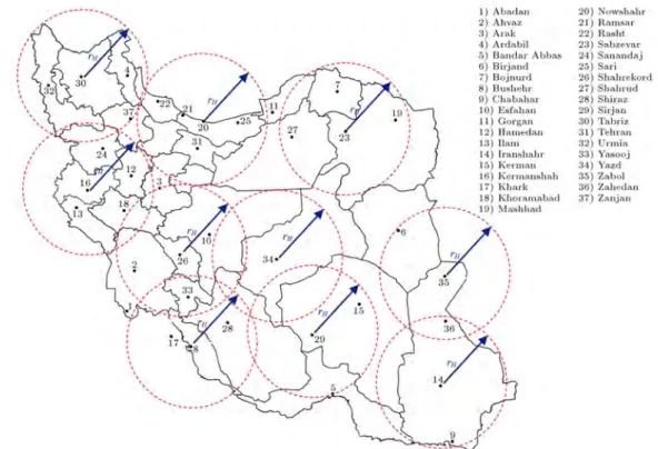
Figure 19 shows the map of 37 nodes on the map of Iran. This map was also presented in Karimi [17]. We denoted the potential nodes of central hubs and hubs by squares and circles, respectively.
Whereas the covering restrictions decrease the CPU times, imposing time bound constraints increases
the computational times in all instances; for example, when = 2880, all reduction factors are 0.9 and PC = 3, the computation times get worse and are equal
to 134.20s. But, when changes to innity, the CPU time decreases one hundred units and is equal to 34.99s. The computational times procedure with the best resolution for IAD data is depicted in Figure 18. These improvements are so eective that they overshadow the poor increasing procedure of costs. The total costs for IAD data are reported in Table 11.
= 1 = 1 = 3000 = 2880
(0.9, 0.9, 0.9, 0.9)
1 143.21 159.66 217.65
-2 139.21 150.84 159.66 159.66
3 136.60 147.19 150.60 154.61
4 135.32 143.44 143.44 143.44
(0.8, 0.8, 0.8, 0.8)
1 135.43 147.43 147.43 147.43
2 130.33 138.97 138.97 138.97
3 128.02 135.71 135.71 135.71
4 126.67 132.38 132.38 132.38
(0.9, 0.8, 0.9, 0.8)
1 143.21 159.66 217.65
-2 136.39 148.03 157.27 157.27
3 132.24 142.18 144.74 144.74
4 130.33 136.46 136.46 136.46
Table 12. The results for IAD data with n = 37 and two central hubs in Tehran and Esfahan.
PH (rH; rC) Cost Hubs CPU time
3000 9
(1; 1)
133.419 2, 5, 10, 12, 23, 30, 31, 33, 34 6.155 10 132.950 2, 5, 10, 12, 22, 23, 30, 31, 33, 34 7.770 11 132.635 2, 5 10, 12, 22, 23, 25, 30, 31, 33, 34 10.416 12 132.369 2, 5, 10, 12, 14, 22, 23, 25, 30, 31, 33, 34 12.600 13 132.144 2, 5, 10, 12, 14, 17, 22, 23, 25, 30, 31, 33, 34 12.759 14 131.928 2, 5, 10, 12, 14, 17, 22, 23, 25, 27, 30, 31, 33, 34 14.369 15 131.719 2, 3, 5, 10, 12, 14, 17, 22, 23, 25, 27, 30, 31, 33, 34 14.591 16 131.552 2, 3, 5, 10, 12, 14, 17, 22, 23, 25, 27, 30, 31, 33, 34, 37 15.612
3000 9
(479, 1390)
142.728 10, 12, 14, 17, 23, 29, 30, 31, 35 1.560 10 138.530 2, 10, 12, 14, 23, 29, 30, 31, 33, 35 1.638 11 136.053 2, 5 10, 12, 14, 23, 30, 31, 33, 34, 35 1.580 12 135.084 2, 5, 10, 12, 14, 22, 23, 30, 31, 33, 34, 35 1.649 13 134.607 2, 5, 10, 12, 14, 17, 22, 23, 30, 31, 33, 34, 35 1.865 14 134.277 2, 5, 6, 10, 12, 14, 17, 22, 23, 30, 31, 33, 34, 35 1.828 15 133.961 2, 5, 6, 10, 12, 14, 17, 22, 23, 25, 30, 31, 33, 34, 35 2.099 16 133.746 2, 5, 6, 10, 12, 14, 17, 22, 23, 25, 27, 30, 31, 33, 34, 35 2.621
4.6. The problem with two central hubs located in Tehran and Esfahan for IAD data We explained the problem with all nodes in IAD data, where PC= 2, so that the central hubs are located only
in Tehran and Esfahan, because memorable cities are 10 and 31 in Table 9, and appear as central hub and hub nodes in more than 92% instances. On the other hands, Esfahan and Tehran are the Islamic capital of the world and Iran's capital, respectively. We considered all nodes as a potential set of hubs, therefore, we
dened H = ^H = 0:9, C = ^C = 0:8, = 3000,
rH = f479; 1g, rH = f1390; 1g and PH = 9 to 16
similar to work done by Yaman [15], as we wanted to have readers compare it with our work. These results are depicted in Table 12. We displayed the procedure of CPU time with a better resolution in Figure 15.
We observed that the results are equal for each PH in dierent amounts of . The outcome of the
problem is depicted on Iran's map for IAD data, and two central hub nodes are xed in cities 10 and 31,
Figure 20. The hierarchical hub network for IAD data with PH= 9, rH= rC= 1 and = 3000.
Figure 21. The hierarchical hub network for IAD data with PH = 9, rH= 479, rC= 1390 and = 3000.
where n = 37 (i.e. set of H equals set of I), PH = 9
and = 3000 in Figures 20 and 21 with rH= rC= 1,
and rH = 479, rC = 1390, respectively. According to
the above conditions, Figure 22 has been presented for the CPU times, which represents the interval run time in the two situations.
5. Conclusion
In this paper, we studied a single assignment hierarchi-cal hub covering problem over a complete network at the rst level, and star networks in the second and third levels. We presented a mixed integer programming
Figure 22. The CPU time of IAD data with n = 37, = 3000 and two central hubs in Tehran and Esfahan for rH = f479; 1g and rH = f1390; 1g.
formulation of the problem and, in order to rapidly solve the model on data sets, a heuristic method for calculating amounts of covering radii was proposed. The proposed model and innovative method are intro-duced in the literature for the rst time. Our model has also considered the subject importance of fairness in providing services, which is signicantly important in the area of servicing; so that, today, in addition to the general time limit (i.e. ) for providing various services, the time for providing primary care services or low level services has a certain individual limit. We tested the model on the CAB, the Turkish network and the IAD data sets, and compared the productivity of the model with that of the basic model on the data sets and understood that it produces ecient solutions with less CPU time. In addition, we did not notice considerable eects on the total routing cost.
References
1. Sahin, G. and Sural, H. \A review of hierarchical facility location models", Computers and Operations Research, 34, pp. 2310 -2331 (2007).
2. O'Kelly, M.E. \A quadratic integer program for the location of interacting hub facilities", Eur. J. Oper. Res. 32(3), pp. 393-404 (1987).
3. Aykin, T. \Ntworking policies for hub-and-spoke tems with application to the air transportation sys-tem", Transport. Sci., 29(3), pp. 201-221 (1995).
4. Campbell, J.F. \Hub location and the p-hub median problem", Oper. Res, 44(6), pp. 923-935 (1996).
5. Ernst, A.T. and Krishnamoorthy, M. \Ecient algo-rithms for the uncapacitated single allocation p-hub median problem", Location Science, 4(3), pp. 139-154 (1996).
6. O'Kelly, M.E., Bryan, D., Skorin-Kapov, D. and Skorin-Kapov, J. \Hub network design with singleand multiple allocation: a computational study", Location Sci., 4(3), pp. 125-138 (1996).
7. Skorin-Kapov, D., Skorin-Kapov, J. and O'Kelly, M.E.
8. Campbell, J.F. \Integer programming formulations of discrete hub location problems", Eur. J. Oper. Res., 72, pp. 387-405 (1994).
9. Kara, B.Y. and Tansel, B.C. \The single-assignment hub covering problem: Models and linearizations", Journal of the Oper. Res. Society, 54(1), pp. 59-64 (2003).
10. Wagner, B. \Model formulations for hub cover-ing problems", Workcover-ing Paper, Institute of Oper-ations Research, Darmstadt University of Technol-ogy, Hochschulstrasse 1, 64289 Darmstadt, Germany (2004).
11. Ernst, A.T., Jiang, H. and Krishnamoorthy, M. \Re-formulations and computational results for uncapaci-tated single and multiple allocation hub covering prob-lems", Unpublished Report, CSIRO Mathematical and Information Sciences, Australia (2005).
12. Tan, P.Z. and Kara, B.Y. \Hub covering model for Cargo delivery systems", InterScience. Networks, 49(1), pp. 28-39 (2007).
13. Calik, H., Alumur, S.A., Kara, B.Y. and Karasan, O.E. \A tabu-search based heuristic for the hub covering problem over incomplete hub networks", Computers & Operations Res., 36(12), pp. 3088-3096 (200).
14. Elmastas, S. \Hub location problem for air-ground transportation systems with restrictions", MS Thesis, Bilkent Universty, Department of Industrial Engineer-ing (2006).
15. Yaman, H. \The hierarchical hub median problem with single assignment", Transportation Research, Part B, 43(6), pp. 643-658 (2009).
16. Marianov, V. and Serra, D. \Hierarchical location-allocation models for congested systems", Eur. J. Oper. Res., 135, pp. 195-208 (2001).
17. Karimi, H. and Bashiri, M. \Hub covering location problems with dierent coverage types", Scientia Iran-ica, E, 18(6), pp. 1571-1578 (2011).
Biographies
Ehsan Korani obtained a BS degree in Industrial Engineering from Islamic Azad University, Kerman-shah, in 2007, and an MS degree in Industrial Engi-neering from the Department of Industrial EngiEngi-neering at Shahed University, Tehran, Iran, in 2010. His research interests lie in the area of facility location, multiple criteria decision making, vehicle routing prob-lem and optimizations. He is author or co-author of several papers, which have been published and presented in reputable international journals and at conferences.
Engineering from Tehran Polytechnic University, Iran, and his PhD degree from Tarbiat Modares Univer-sity, Tehran, Iran. He is Assistant Professor of Industrial Engineering and Supply Chain Research in the Department of Industrial Engineering at Shahed University, Iran. His research interests include the
development and application of quantitative techniques to the sequencing, simulation and design of supply chain and logistic systems, and to Location-Routing Problems (LRP). He is author and co-author of several papers, which have been published in nationals and international journals.