Vol. 8, No. 1, March 2019, pp. 63~76
ISSN: 2252-8938, DOI: 10.11591/ijai.v8.i1.pp63-76 r 63
An improved radial basis function networks in networks
weights adjustment for training real-world nonlinear datasets
Lim Eng Aik1, Tan Wei Hong2, Ahmad Kadri Junoh3
1,3Institut Matematik Kejuruteraan, University Malaysia Perlis, 02600 Arau, Perlis, Malaysia. 2School of Mechatronic Engineering, University Malaysia Perlis, 02600 Arau, Perlis, Malaysia.
Article Info ABSTRACT
Article history: Received Dec 27, 2018 Revised Feb 17, 2019 Accepted Feb 28, 2019
In neural networks, the accuracies of its networks are mainly relying on two important factors which are the centers and the networks weight. The gradient descent algorithm is a widely used weight adjustment algorithm in most of neural networks training algorithm. However, the method is known for its weakness for easily trap in local minima. It suffers from a random weight generated for the networks during initial stage of training at input layer to hidden layer networks. The performance of radial basis function networks (RBFN) has been improved from different perspectives, including centroid initialization problem to weight correction stage over the years. Unfortunately, the solution does not provide a good trade-off between quality and efficiency of the weight produces by the algorithm. To solve this problem, an improved gradient descent algorithm for finding initial weight and improve the overall networks weight is proposed. This improved version algorithm is incorporated into RBFN training algorithm for updating weight. Hence, this paper presented an improved RBFN in term of algorithm for improving the weight adjustment in RBFN during training process. The proposed training algorithm, which uses improved gradient descent algorithm for weight adjustment for training RBFN, obtained significant improvement in predictions compared to the standard RBFN. The proposed training algorithm was implemented in MATLAB environment. The proposed improved network called IRBFN was tested against the standard RBFN in predictions. The experimental models were tested on four literatures nonlinear function and four real-world application problems, particularly in Air pollutant problem, Biochemical Oxygen Demand (BOD) problem, Phytoplankton problem, and forex pair EURUSD. The results are compared to IRBFN for root mean square error (RMSE) values with standard RBFN. The IRBFN yielded a promising result with an average improvement percentage more than 40 percent in RMSE.
Keywords: Gradient Descent Improved RBFN Neural network
Radial basis function network Weight Adjustment
Copyright © 2019 Institute of Advanced Engineering and Science. All rights reserved.
Corresponding Author: Lim Eng Aik,
Institut Matematik Kejuruteraan, University Malaysia Perlis, 02600 Arau, Perlis, Malaysia. Email: e.a.lim80@gmail
1. INTRODUCTION
The term Radial Basis Function networks (RBFN) is associated with radial basis function (RBF) in single-layered networks with structure as shown in Figure 1. Radial Basis Function (RBF) Networks derived from the theory of function approximation. It was originally used in exact interpolation in multidimensional space by Moody and Darken [1]. RBFN displayed its advantages over other types of neural networks with better approximation abilities, simple network design and faster learning algorithms.
Consequently, RBFN becomes a popular tools among researchers for many applications such as classification, pattern recognition and approximation model.
Numerous researchers whom have been working to improves RBFN training algorithms, set alongside the standard techniques [2–8]. RBFN are useful in approximation problems, but it is time-consuming to train the networks as it connect to a large numbers of training data, nonetheless generate high error due to possible invalid data or designation of weights in hidden layer. Although a standard RBFN has been proved by Sarimveis [2] to be faster in training with reasonable accuracy, it still produces substantial error. Such outcomes were caused by the standard RBFN that lack the ability to computes accurate weights for hidden layer that able to represent the level of importance for each hidden nodes. Through improving the weights calculation equation in standard RBFN during updating stage, we can fix the problem stated above.
Noted that the more accurate the weights are assigns to each node, more accurate the information that feeds to the output layer of network, resulting in accurate results. In this paper, an improved RBFN that outperforms the standard RBFN in term of accuracies is presented. The proposed networks efficiency is demonstrated through the application of eight experimental models, with four nonlinear model from literatures, three real-world problems data obtained from Lim [9] and one real-world time-series data from XM metatrader 4 trading platform [10]. The advantages of the presented proposed networks are identified and the results are compared with standard RBFN and discussed.
Figure 1. The architecture of RBFN
2. RELATED WORKS
Radial basis function networks (RBFN) are well-known for its ability to generalize and approximate a sample data without the requirement for the equation and coefficients, particularly when an unknown model describing an unknown complex relation with abundant training data. Due to their ability to generalize substantially, RBFN are usually selected for this purpose [11-23]. Furthermore, in this big data era, many domains such as image processing, text categorization, biometric, microarray, etc. had the size of datasets so large, that real-time system requires long time and memory storage to process them.
Under the same group, the backpropagation neural networks also can generalize and approximate complex dataset. However, due to the architecture of backpropagation neural networks that works in forward and backward direction, delays in training time is unavoidable. Furthermore, in term of approximation, multiple literatures showed that the RBFN is more superior than backpropagation neural networks, in term of training speed and accuracy [24-28]. Two main criteria that determine the accuracy of an RBFN are the initial centre and the networks weights. In this paper, we focus mainly on networks weight adjustment. Throughout many literatures, we found that weight adjustment in RBFN play vital role in determine
x1
x2
x3
xN
.
.
.
.
.
.
Input layer Hidden Layer of RBF Output Layer
ψ
ψ
ψ
ψ
wN
.
.
.
w2
w3
its accuracy in approximation problem. Wang et al. [29] study the effectiveness of extreme learning machine by adjusting its networks weights, it is found that networks weight significantly inflicts in output accuracy. A year after Wang’s team finding, Hadi et al. [30] proof the weak robustness in multilayer perceptron and RBFN in estimating large dataset was due to the lack in weight correction algorithm in both the networks. The work related to weight correction is then supported by Godoy et al. [31] and Sodhi et al. [32] that proof when a better weight is assigned to the networks, the output yield significantly better in accuracy. Recently, Cao et al. [33] in their review work, stated that random weight approaches in RBFN causes the reduce the network accuracy in most approximation case studies.
In finding solution to obtained better weights adjustment and gaining accurate approximation, Navarro et al. [34,35] demonstrated that the hybrid of evolutionary algorithm such as particle swarm optimization (PSO) with RBFN shows a good performance in classification problems and approximation problems. This work is extended by Leung et al. [36, 37] by introducing a novel PSO method or adjusting the RBFN networks weight. Moreover, the following years, evolutionary algorithm turn popular and becoming the focus tools for weight adjustment in RBFN, where the combination of multiple evolutionary algorithm such as genetic algorithm and PSO with RBFN [38, 39]. Some researcher uses a modified version of genetic algorithm as networks weights controller for gaining better results [40-42] and most recent on using modified PSO in RBFN for weight adjustment by Mirjalili [11]. The used of evolutionary algorithm as a tool for network weights adjustment in RBFN training was indeed a good method if the networks training speed and computation cost are not main concerns.
Alongside with used of evolutionary algorithm, there are also some research on using fuzzy inference rule as weight setting for RBFN which yield good results [43, 44]. However, the application of fuzzy inference in RBFN was only tested in classification problem, and the setting of the fuzzy rule is a challenging task for regular researchers that do not have fuzzy theory background. In contrary, the used of statistical method in obtaining suitable weight for RBFN were reported in numerous literatures [45-48], that uses stochastic method, Grover searching algorithm, Hierarchy Markovian matrix and attributed class correlation method for that purposes. Furthermore, it is also reported that the learning algorithm for networks training may perform worse with the increases of dataset [49]. Incorporating statistical method into RBFN is a complicated task, requires deep understanding in flow of algorithm and statistical theory to implement such approaches. Furthermore, the reported improvement on results in mentioned literatures are not significant enough for the complicated implementation process involved. Moreover, there are others studies using extreme learning machine as tool for weight adjustment shown by Tang and Huang [50] and, Dash and Dash [51]. Both studies used extreme learning machine for controlling the networks weights during training process. There are numerous others less known method used for RBFN weight adjustment are projection based learning method [52], linear interval regression weights method [53], self-organized RBFN based on mutual information and neurons activity [54], novel two-steps algorithms [55], self-constructing least-Wilcoxon method [56], and semi-analytic computation of Laurent series [57].
Finally, researcher also incorporating part of backpropagation neural networks algorithm that involved the weight updating stage into RBFN to enhance the performance of weight correction ability in the algorithm. In 2011, Philip et al. [58] used feed forward neural network to correct the weight for backpropagation neural networks during learning stage. In the same year, Malviya et al. [59] used backpropagation neural network and PSO as weight tuning tool for RBFN. Since then, many research focuses on gradient descent (GD) algorithm were proceeds with good results, as GD algorithm was the weight updating algorithm in backpropagation neural networks.
In 2012, Mohseni et al. [60] introduced a mixed training algorithm using backpropagation neural networks and variable structure system to optimize weight updating in RBFN. Assaf et al. [61] then proposed a new training mode using unsupervised classification algorithm where the connections of weights are learned using GD algorithm. Then Xie et al. [62] further extended the uses of GD algorithm to second order GD algorithm in training RBFN where the weight is adjusted during training. Though the GD algorithm is a great approaches for finding weight, however, the GD algorithm also has weakness such as easily trap in local minima [63, 64].
To overcome the weakness of GD algorithm, a few studies were done. Ganapathy et al. [65] demonstrated the efficiency of an improved steepest descent algorithm for determining weight of hidden layer to output layer network. Chang et al. [21] proposed the used of error feedback scheme in RBFN for weight correction which can avoid the local minima problem. Recently, Mohammadi et al. [16] applied a pseudo-inverse algorithm for calculating weight updating matrix even with large dataset that can fix the local minima problem. In the mentioned literatures, clearly most approaches involved complicated process to perform the computation and some approaches yield not significant improvement in accuracies. Furthermore, many approaches focus on applying separate part of methods or algorithm for weight adjustment instead of focusing on improving RBFN internal algorithm. In this paper, we focus on improving
the internal algorithm for weight correction stage and reduce complicated algorithm which in turn making RBFN algorithm precede faster computation with low computation cost. This paper is organized with the following section describing the standard RBFN, follows by steps in improving the standard RBFN and used for simulating and predicting the eight experimental models. Then, in section 4 discussed the results of each models and compared with standard RBFN for accuracies. Finally, section 5 concludes the findings and discussed some future work that would help in improving the proposed improved RBFN.
3. METHODOLOGY
3.1. Radial basis function network (RBFN)
RBFN is an intelligent interpolation technique for modeling a linear or nonlinear multidimensional data. RBFN is often used for prediction problems. Its kernel has two parameters; the center and its radius. These two parameters can determined through unsupervised or supervised learning as proposed by Moody and Darken in 1989 [1]. RBFN is a type of feed-forward neural network. The network structure consists of three-layer network similar to multi-layer feed-forward network. In the network structure of RBFN as shown in Figure 1, the first layer is the input layer and is composed of signal source nodes. The second layer is a hidden layer, and the number of nodes of the layer is determined by the nature of the problem to be solved and the characteristics of the specific problem. The transfer function of the neurons in this layer is the radial basis function, which is a global function that responses as the forward network transformation function. The third layer is the output layer, which responds to the input layer.
The main idea of the RBFN is to use the radial basis function as the "base" of the hidden layer unit to build the hidden layer. In the hidden layer, the input vector is transformed. Thus, low-dimensional input data can convert to a high-dimensional space. Such approach can transform a linearly inseparable problem in a low-dimensional space into a linearly separable in a high-dimensional space, thereby solving the related problem. RBFN training is simple and has fast learning convergence. It can approximate any nonlinear function. Therefore, the RBFN has a extensive applications in pattern recognition, image processing, predictions and nonlinear control. From the perspective of function approximation, RBFN are local approximations. If the number of neural units in the hidden layer reaches a certain level, the network can approximate any continuous function with arbitrary precision. In addition, due to RBFN adopts a linear mapping relationship between the output layer and the hidden layer; the network can avoid the complicated back-propagation operation as in back-propagation neural network. Therefore, in RBFN, the speed of operation and the accuracy of nonlinear fitting are improved. During the operation to solve a problem, the RBFN has the characteristics of the training samples corresponding to the radial basis function mapping, resulting in a large amount of network computation, and may cause problems in solving the networks weights.
3.2. RBFN model and learning algorithm
The RBFN by default uses the Gaussian function as the kernel function of the hidden unit (1).
( )2
2 i ik i
k
X C
k
r e σ
− −
∑
= (1)
Where rk is the output value of the k-th Gaussian unit of the hidden layer; C is the i-th input variable value of the center of the kernel of the k-th Gaussian unit;
σ
k is the spread of the kernel of the k-th Gaussian unit.The supervised learning rule used to adjust the link weighting value between the hidden unit and the output unit, and the threshold value of the output unit. The difficulty with RBFN determines the number of hidden units and the center of the Gaussian function and the radius parameters. The two parameters, center and radius, can determined by supervised or unsupervised learning. The supervised learning of RBFN is similar to back-propagation, and the learning rules can derived by minimizing the sum of squares errors and the gradient descent method. Unsupervised learning uses the K-means algorithm to find the cluster center of the sample as the center of the Gaussian function of each hidden unit. Though RBFN has an extensive applications in pattern recognition, predictions, and control system, the algorithms still a disadvantage on an independent variables have the same position, so the contour of the kernel function is circular. However, each independent variable has different influence on the dependent variable, and the contour of the kernel function should be elliptical.
3.3. RBFN implementation, advantages and limitation
The implementation of the RBF neural network consists of two parts: the network structure part and the algorithm parameter part. The network structure is designed to determine the number of nodes in the hidden layer of the network. The part of the algorithm parameters is determined for the three important parameters of the data center of the radial basis function, the spread constant and the output layer weight. Since the number of hidden layer nodes is consistent with the number of samples, and the center of the radial basis function is the sample itself, only the spread constant and the output layer weight need to be determined when establishing the network. However, when building an RBFN, the learning algorithm needs to solve more problems, including the determination of the number of hidden layer nodes, the determination of the data center of the radial basis function, the spread constant, and the correction of the weights of the output layer. The establishment and training of the radial basis function neural network is composed of two stages. The first phase primarily determines the data center of the radial basis function in the hidden layer, typically used as the center's self-organizing selection method for unsupervised learning processes. The input samples are clustered to determine the center of the radial basis function of the hidden layer nodes.
The RBFN has its adaptive ability and fault tolerance. Therefore, while dealing with the complex evaluation of nonlinearity, the factors that have no significant influence on the evaluation results can effectively eliminated. The RBFN is improved via the supervised learning rules are used to adjust the link weighting value between the hidden unit and the output unit, and the threshold of the output unit. The learning rule is derived by minimizing the sum of squared errors and the gradient descent method. 3.4. Improved RBFN (IRBFN)
RBFN were reported has an extensive applications and its algorithms have many different variants [11, 19, 66, 67]. Yeh and Chen [68] proposed an improved RBFN with kernel shape parameters to derive its learning rules in supervised learning, which is superior to conventional RBFN. It is proved that after the kernel function is given the weight; the shape of the kernel function is elliptical, which is more reasonable than the shape of the circular kernel function which has the same position as all the independent variables of the conventional RBFN. Therefore, this proposed improved RBFN is reasonably has superior fitting degree than conventional RBFN.
During the forward propagation of proposed network, which is also known as recall stage, the calculation of the hidden layer output vectors requires (2) and (3).
(
)
exp
k k
h = −net (2)
(
)
22
2 , 1, 2, 3,...,
ik i ik i
k
k
V x C
net k N
σ −
= =
∑
(3)
where xi is the i-th input value; hk is the output value of the k-th Gaussian unit of the hidden layer; netk is
the net value of the k-th Gaussian unit of the hidden layer; Cik is the i-th input variable value of the center of the kernel of the k-th Gaussian unit; Vik is the weighted value of the i-th input variable of the kernel of the k-th Gaussian unit, representing k-the importance of k-the input variable;
σ
k is the radius of the kernel of the k-th Gaussian unit.During the network training process,
σ
kmay adjusted to 0, causing the denominator to be 0.In order to avoid this trouble, (3) is modified to the following formula.
(
)
22 2
, 1, 2, 3,...,
k k ik i ik i
net =Q
∑
V x −C k= N (4)where Qk is the reciprocal of the radius of the kernel of the k-th Gaussian unit. In calculating the responded output vector, (5) is used.
(
)
1 1 exp
j
j
y
net
=
+ − (5)
j kj k j k
net =
∑
W h −θ
(6)where netj is the net value of the j-th unit of the output layer; yj is the output value of the j-th
output unit; Wkj is the connection weight between the k-th unit of the hidden layer and the j-th unit of the
output layer; θj is the threshold of the j-th unit of the output layer.
Now for backward propagation, which is the learning stage, as this supervised learning aims to reduce the difference between the target output value of the network output unit and the responded output value, the quality of learning is generally expressed by the following cost function:
(
)
21
2 j j
E=
∑
t −y (7)where tj is the target output value of the j-th output unit of the training sample output layer;
j
y
is the responded output value of the j-th output unit of the training sample output layer.
Since the cost function is a function of the responded output value, and the responded output value is a function of the network connection weight value and the parameters of the center and radius of the Gaussian unit, the cost function is a function that links the weight value and the Gaussian unit parameter. Therefore, adjusting the link weight value and the Gaussian unit parameter can change the size of the cost function. In order to minimize the cost function, the gradient descent method is used to adjust the network link weighting value and the Gaussian unit parameter.
The following is divided into two parts to derive the correction formula. 1. The weighted value of the link between the hidden layer and the output layer. 2. The Parameters of the Gaussian unit in hidden layer.
To find the weighted value of the link between the hidden layer and the output layer, the correction weight of the link weight between the network output layer and the hidden layer is the same as the inverse gradient descent algorithm, but it is still fully derived here. First, get the partial differential law:
j j
kj
kj j j kj
y net
E E
W
W y net W
η
∂η
∂ ∂ ∂Δ =− =− ⋅ ⋅
∂ ∂ ∂ ∂
(8)
Where,
(
)
2(
)
1
2 j j j j
j j
E
t y t y
y y
∂ ∂
= − =− −
∂ ∂
⎛
⎞
⎜
⎟
⎝
∑
⎠
(9)
(
)
(
)
j
j j
j j
y
f net f net net
∂ ∂
ʹ
= =
∂ ∂
(10)
j
kj k j k k
kj kj
net
W h h
W W
θ
∂ ∂
= − =
∂ ∂
⎛
⎞
⎜
⎟
⎝
∑
⎠
(11)(
)
(
)
(
)
kj j j j k j j j k
W
η
t y f hʹη
t y f hʹΔ =− ⋅ − − ⋅ ⋅ = ⋅ − ⋅ ⋅ (12)
Define,
(
)
(
)
(
)
j
j j j j j j j
j j j
y
E E
t y f t y f
net y net
δ
=− ∂ =− ∂ ⋅ ∂ =− − − ⋅ ʹ= − ⋅ ʹ∂ ∂ ∂
(13)
Therefore, (12) can rewritten as,
kj j k
W
η δ
hΔ = ⋅ ⋅ (14)
Hence, the correction of threshold value also can rewritten as,
j j
j
E
θ
η
ηδ
θ
∂
Δ =− =−
∂ (15)
For Parameters of the hidden layer Gaussian unit, the central value correction of the kernel of the Gaussian unit can obtained by the partial differential law:
k ik
ik k ik
net
E E
C
C net C
η
∂η
∂ ∂Δ =− =− ⋅
∂ ∂ ∂
(16)
Where,
k k
k j
k k k k k
h net
E E E
f
net h net net h
∂ ∂
∂ ∂ ∂
ʹ
= ⋅ = ⋅
∂ ∂ ∂ ∂ ∂
⎛
⎞
⎜
⎟
⎝
∑
⎠
(17)Due to (13),
j
j E net
δ
=− ∂∂ (18)
This turn (17) into,
(
j kj)
k j kjj j
k
E
W f W f
net
δ
δ
∂
ʹ ʹ
= − ⋅ =− ⋅
∂
⎛
⎞
⎛
⎞
⎜
⎟
⎜
⎟
⎝
∑
⎠
⎝
∑
⎠
(19)Now we define,
k j kj k
j
W f
δ
=⎛
⎜
δ
⋅⎞
⎟
⋅ ʹ⎝
∑
⎠
(20)Therefore,
k k
E net
δ
∂=−
(
)
2(
(
)
)
2 2 2 2
2
k
k ik i ik k ik i ik
i i
ik ik
net
Q V x C Q V x C
C C ∂ ∂ = − = − − ∂ ∂
⎛
⎞
⎜
⎟
⎝
∑
⎠
∑
(22)Now, we substitute (21) and (22) into (16), we obtained,
(
)
2 2(
(
)
)
2 2(
)
2 2
ik k k ik i ik k k ik i ik
i
C
η
δ
Q V x Cηδ
Q V x CΔ =− ⋅ − ⋅ − − =−
∑
− (23)Similarly, the mutual correction of the radius of the kernel of the Gaussian unit can obtain by a partial differential law:
k k
k k k
net E E Q
Q net Q
η
∂η
∂ ∂Δ =− =− ⋅
∂ ∂ ∂ (24)
where,
(
)
2(
)
22 2 2
2 k
k ik i ik k ik i ik
i i
k k
net
Q V x C Q V x C
Q Q ∂ ∂ = − = − ∂ ∂
⎛
⎞
⎜
⎟
⎝
∑
⎠
∑
(25)By substituting (21) and (25) into (24), we obtained,
(
)
2(
)
2 2(
)
22 2
k k k ik i ik k k ik i ik
i i
Q η δ Q V x C ηδQ V x C Δ =− − ⋅
⎛
⎜
−⎞
⎟
= −⎝
∑
⎠
∑
(26)Similarly, the weight of the input variable weight (shape parameter) of the Gaussian unit can obtained by the partial differential law:
k k
k k k
net
E E
V
V net V
η
∂η
∂ ∂Δ =− =− ⋅
∂ ∂ ∂ (27)
Where,
(
)
2(
)
22 2 2
2 k
k ik i ik k ik i ik
i i
k k
net
Q V x C Q V x C
V V ∂ ∂ = − = − ∂ ∂
⎛
⎞
⎜
⎟
⎝
∑
⎠
∑
(28)By substituting (21) and (28) into (27), we obtained,
(
)
2(
)
2 2(
)
22 2
k k k ik i ik k k ik i ik
i i
V η δ Q V x C ηδ Q V x C
Δ =− − ⋅
⎛
⎜
−⎞
⎟
= −⎝
∑
⎠
∑
(29)The five (14) ,(15), (23), (26) and (29) are the learning rules of the improved RBF neural network. Clearly, from above derivation equations, there is one more shape parameter in the tunable parameter than the conventional RBFN. The supervised learning rules of all parameters are uniformly derived by using the principle of sum squares error minimization, including the center, radius, and shape parameters of the kernel function, the weighting value of the networks between the hidden unit and the output unit, and the threshold of the output unit.
The RBFN is often used for prediction and classification problems, but it has the disadvantage that all independent variables have equal status, with the shape of the kernel function is circular and this influence outcome the networks. Since the weights of each input are different, so the shape of the kernel function should be elliptical. To overcome this shortcoming, an improved RBFN with kernel shape parameters is
proposed, and its learning rules are derived by supervised learning. This architecture is superior to traditional radial basis function networks.
Clearly, from Figure 2 that based on the RBFN, the proposed IRBFN has the weight of V added between the input layer and the hidden layer to indicate the influence of different input layer units on the hidden layer unit, which later use for calculating the weights of hidden layer to output layer.
Figure 2. The architecture of IRBFN 4. RESULTS AND DISCUSSION
The proposed IRBFN was tested using 4 nonlinear function from literatures, which are Santner et al. [69] function given in (30), Lim et al. [70] function in (31), Dette and Pepelyshev [71] function in (32), and Friedman [72] function in (33). For all these 4 functions, the training set for RBFN consists of 400 sets of random generated data points and test set comprises 400 sets of random generated data points, both in range of [0,1].
[ ]
( ) exp( 1.4 ) cos(3.5 ), 0,1
f x = − x
π
x x∈ (30)( )
[
(
1(
1)
)
(
(
2)
)
]
[ ]
1
30 5 sin 5 4 exp 5 100 , 0,1 , 1, 2.
6 i
f x = + x x + − x − x ∈ ∀i=
(31)
( )
(
2)
2(
)
2(
)
2[ ]
1 2 2 2 3 3
4 2 8 8 3 4 16 1 2 1 , i 0,1 , 1, 2, 3.
f x = x − + x − x + − x + x + x − x ∈ ∀i= (32)
( )
(
)
(
)
2[ ]
1 2 3 4 5
10sin 20 0.5 10 5 , i 0,1 , 1, 2, 3, 4, 5.
f x =
π
x x + x − + x + x x ∈ ∀i= (33)IRBFN was also tested on 4 real-world datasets for its performance. The Biochemical Oxygen Demand (BOD) concentration dataset, phytoplankton growth rate and death rate dataset and air pollutant dataset were obtained from Aik and Zainuddin [73]. Another which is the dataset from forex for EURUSD pairs is collected from XM Metatrader 4 database [10]. The BOD dataset and phytoplankton dataset both consists of 100 sets of data and the test set comprises 100 sets of data. Meanwhile, for air pollutant dataset, the training set has 480 sets of data and the test set has 72 sets of data, which both were taken from hourly air
x1
x2
x3
xN
.
.
.
.
.
.
Input layer Hidden Layer of RBF Output Layer
ψ
ψ
ψ
ψ
wN
.
.
.
w2
w3
w1
V11
V12
V13
V14
V21 V 22
V23
V24
V31
V32
V33
V34
VN1
VN2
VN3
data. For EURUSD pairs, the training set consists of 519 sets of data taken from year 2016 to end of year 2017. The test set consists of 155 sets of data taken from early year 2018 to August 2018.
The experiment was implemented by using the newrb function because it represents the general form of an RBF network. Furthermore, the proposed clustering method has been implemented by using MATLAB’s function. Gaussian basis function has been used for both networks with other parameters such as spread was set to default value, so the performance of the proposed network can evaluated effectively [8]. Performance of standard RBFN and IRBFN in this experiment has been measured by comparing the computation time taken for training with number of iteration taken for convergence and the Root Mean Squared Error (RMSE) to measure how well both networks approximates the chosen functions and it is given by.
(
)
2 11 n
i i i
RMSE O P n =
=
∑
−where n is the number of predicted responder; Oi is the target value for time-step i, and Pi is the predicted
value of the model at time-step i.
The number of centers for RBFN is fixed to 10 centers for all 8 datasets training. For air pollutant problem, the pollutant monitored includes carbon monoxide, nitric oxide, nitrogen dioxide, ozone, and oxides of nitrogen. For experimental purposes, hourly updated air quality data obtained from Aik and Zainuddin [73] has been used to predict the trend of interested pollutants for Nitric Oxide, Nitrogen Dioxide and Oxides of Nitrogen. While for Phytoplankton problem, growth rate and death rate have been used as the interested values. As for the BOD problem, the BOD concentration has been taken as the interested value. Finally, the forex EURUSD dataset consists of three variables is taken considered for training, which are the daily highest price, daily lowest price and open price, while the close price is used for prediction.
Table 1. Performance of IRBFN and Standard RBFN prediction results for datasets
Dataset
Standard RBFN IRBFN
Average of RMSE Standard Deviation of RMSE Average of RMSE Standard Deviation of RMSE
Santner 0.160980 0.132510 0.095935 0.021740
Lim 0.151190 0.053404 0.094039 0.011824
Dette 1.938260 1.318204 0.952562 0.175806
Friedman 1.333590 0.700492 0.162113 0.058887
BOD 0.000252 3.87e-07 0.000247 4.29e-05
Phytoplankton 0.004980 0.000933 0.004035 0.000800
Air Pollutant 4.203630 2.860265 0.371875 0.109962
EURUSD 0.031649 0.004812 0.028432 0.004942
Table 2. Percentage of Improvement for IRBFN over Standard RBFN by RMSE
Dataset Percentage of Improvement (%)
Santner 40.41
Lim 37.80
Dette 50.85
Friedman 87.84
BOD 1.80
Phytoplankton 18.98
Air Pollutant 91.15
EURUSD 10.16
Results from Table 1 shows that IRBFN networks outperform standard RBFN in average RMSE and standard deviation of RMSE. All results of average RMSE in Table 1 are calculated using ten times run of each networks. From Table 1, IRBFN network surpasses the standard RBF in accuracy and network architecture by using training set which consists only 81.8%, 71.8%, 68.5%, and 65.8% of total dataset size for Santner dataset, Lim dataset, Dette dataset, and Friedman dataset, respectively. While IRBFN network training for real-world dataset involves the BOD dataset, Phytoplankton dataset, Air pollutant dataset and forex EURUSD dataset used only 81.8%, 71.8%, 68.5% and 66.8%, respectively. This means that, it is possible to suitable number of dataset such that, it will provide a network with reduced complexity, faster training time and improved accuracy. Table 2 shows the results of the percentage of improvement of RMSE
for IRBFN network in compared to standard RBFN. Results showed that IRBFN network outperform standard RBFN network in term of accuracy more than 80% for Friedman dataset and air pollutant dataset. Meanwhile, for Santner dataset, Lim dataset and Dette dataset each obtained improvement in range of 37% to 51%. However, BOD dataset shows no significant improvement for IRBFN network over standard RBFN with percentage less than 2%. This is due to the high nonlinearity of BOD data, besides, the lack of additional input variable that control the changes in BOD can lead to weak prediction results.
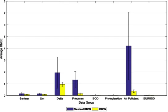
The results from real-world datasets for Phytoplankton dataset and forex EURUSD dataset showed improvement of 18.98% and 10.16%, respectively. Both of this datasets are highly nonlinear data. Possible existence of other environmental factor that not included in dataset possibly is the reason behind the low improvement percentage occurs for Phytoplankton dataset. Additionally, for forex EURUSD dataset, the low improvement percentage is due to many possible factors not included in the dataset that also drives the movement of this currency values. Factor that cannot be quantified, such as political influences or natural disaster, can affect the currency fluctuation. Hence, if such factors can quantify and includes in the dataset, improvement in percentage is expected. From Table 1 and Table 2, we observed that IRBFN network provide such consistent results even that it uses less dataset and still able to perform such satisfying results. The results of prediction from IRBFN network are consistent as we observed from Table 1, the standard deviation of RMSE was much lower than standard RBFN. Figure 3 shows the error bar plot that displayed the comparison of errors for both the networks. Clearly, the standard RBFN has larger error in compared to IRBFN network for all datasets.
Figure 3. Error bar plot for datasets using standard RBFN and DWKM-RBFN
The IRBFN network and Standard RBFN performed well in the experiments for dataset with smaller range that lies in [0,1]. However, for larger range of dataset such as air pollutant dataset, the standard RBFN performed poorly in accuracy. Besides, the IRBFN network is superior in accuracies but a proper adjustment in the hidden layer weightage can enhance the networks accuracy to much higher level. The results in Table 1 shows that even with less dataset used for training, if the right weights are assigned, can impact in prediction accuracy. The uses of huge number of dataset does not always guarantee the desirable prediction accuracies, but sufficient number of dataset that can represent the shape of the distribution for the dataset is enough for providing good prediction results. Furthermore, a large number of training dataset might contain invalid data that could jeopardize the desired accuracy, not mentioning the size of network it would create and the time taken for training. Hence, there is no denial on the ability of the IRBFN network and standard RBFN in prediction, but it comes with a hefty compensation for the accuracy if the proper value of hidden layer weights is not assigned. As the number of datasets for the network becomes lesser and it results much simpler
network architecture and possibly free of invalid dataset. Although both models provide satisfying results, the network structure and accuracy of the IRBFN network is superior compared to the standard RBFN network.
5. CONCLUSION
Four literatures nonlinear functions and four real-world problems have been simulated in this paper, where we applied for real-world problems on prediction of BOD problem, phytoplankton problem, air pollution problem and forex EURUSD price prediction problem. The performance of both networks has been compared to the case using the Root Mean Squared Error (RMSE) and standard deviation as the criteria for performance measurement and network prediction consistency. Results from all eight studies show that the IRBFN network is better than the standard RBFN in prediction accuracy and network architecture. Thus, it is possible to improve the accuracy of the proposed network by using clustering methods to choose the best value of number of center to be used for different type of dataset. As conclusion, the proposed IRBFN is far superior to the standard RBFN network as for network accuracy. Since self-organized selection of centers can performed by clustering algorithms for selecting significant centers, sufficient to represent the distribution of dataset for the hidden nodes has been used, it would be interesting if the networks to be tested with high noise training data with clustering algorithm such as K-means algorithm or fuzzy C-means algorithm as center selector to verify the efficiency of the IRBFN.
REFERENCES
[1] J. Moody and C. J. Darken, “Moody, J., & Darken, C. J. (1989). Fast learning in networks of locally-tuned processing units. Neural Computation, 1, 281-294.,” Neural Comput., vol. 1, pp. 281–294, 1989.
[2] H. Sarimveis, A. Alexandridis, and G. Bafas, “A fast training algorithm for RBF networks based on subtractive clustering,” Neurocomputing, vol. 51, pp. 501–505, 2003.
[3] A. Alexandridis, E. Chondrodima, N. Giannopoulos, and H. Sarimveis, “A Fast and Efficient Method for Training Categorical Radial Basis Function Networks,” IEEE Trans. Neural Networks Learn. Syst., pp. 1–6, 2016.
[4] A. Alexandridis, E. Chondrodima, N. Giannopoulos, and H. Sarimveis, “A fast and efficient method for training categorical radial basis function networks,” IEEE Trans. Neural Networks Learn. Syst., vol. 28, no. 11, pp. 2831– 2836, 2017.
[5] Y. Hu, J. J. You, J. N. K. Liu, and T. He, “An eigenvector based center selection for fast training scheme of RBFNN,” Inf. Sci. (Ny)., vol. 428, pp. 62–75, 2018.
[6] E. M. da Silva, R. D. Maia, and C. D. Cabacinha, “Bee-inspired RBF network for volume estimation of individual trees,” Comput. Electron. Agric., vol. 152, pp. 401–408, 2018.
[7] D. Shan and X. Xu, “Multi-label Learning Model Based on Multi-label Radial Basis Function Neural Network and Regularized Extreme Learning Machine,” Moshi Shibie yu Rengong Zhineng/Pattern Recognit. Artif. Intell., vol. 30, no. 9, 2017.
[8] Y. Sun et al., “The application of RBF neural network based on ant colony clustering algorithm to pressure sensor,”
Chinese J. Sensors Actuators, vol. 26, no. 6, 2013.
[9] L. E. Aik, “Modified Clustering Algorithms for Radial Basis Function Networks,” Universiti Sains Malaysia, 2006. [10] L. XM Global, “XM Metatrader 4,” 2018. [Online]. Available: https://www.xm.com/mt4. [Accessed: 20-Jul-2018]. [11] S. Mirjalili, “Evolutionary Radial Basis Function Networks,” in Studies in Computational Intelligence, 2019, pp.
105–139.
[12] A. Osmanović, S. Halilović, L. A. Ilah, A. Fojnica, and Z. Gromilić, “Machine learning techniques for classification of breast cancer,” in IFMBE Proceedings, 2019.
[13] Y. Lei, L. Ding, and W. Zhang, “Generalization Performance of Radial Basis Function Networks,” Neural Networks Learn. Syst. IEEE Trans., vol. 26, no. 3, pp. 551–564, 2015.
[14] C. Arteaga and I. Marrero, “Universal approximation by radial basis function networks of Delsarte translates,”
Neural Networks, vol. 46, pp. 299–305, 2013.
[15] S. Lin, “Linear and nonlinear approximation of spherical radial basis function networks ✩,” vol. 35, pp. 86–101, 2016.
[16] M. Mohammadi, A. Krishna, S. Nalesh, and S. K. Nandy, “A Hardware Architecture for Radial Basis Function Neural Network Classifier,” IEEE Trans. Parallel Distrib. Syst., 2018.
[17] M. W. L. Moreira, J. J. P. C. Rodrigues, N. Kumar, J. Al-Muhtadi, and V. Korotaev, “Evolutionary radial basis function network for gestational diabetes data analytics,” J. Comput. Sci., 2018.
[18] K. Kavaklioglu, M. F. Koseoglu, and O. Caliskan, “International Journal of Heat and Mass Transfer Experimental investigation and radial basis function network modeling of direct evaporative cooling systems,” Int. J. Heat Mass Transf., vol. 126, pp. 139–150, 2018.
[19] M. Smolik, V. Skala, and Z. Majdisova, “Advances in Engineering Software Vector fi eld radial basis function approximation ☆,” Adv. Eng. Softw., vol. 123, no. 17, pp. 117–129, 2018.
[20] Y. Li, X. Wang, S. Sun, X. Ma, and G. Lu, “Forecasting short-term subway passenger flow under special events scenarios using multiscale radial basis function networks,” Transp. Res. Part C Emerg. Technol., 2017.
wind speed and power forecast,” Renew. Energy, 2017.
[22] Q. P. Ha, H. Wahid, H. Duc, and M. Azzi, “Enhanced radial basis function neural networks for ozone level estimation,” Neurocomputing, 2015.
[23] Z. Majdisova and V. Skala, “Radial basis function approximations : comparison and applications,” Appl. Math. Model., vol. 51, pp. 728–743, 2017.
[24] F. Mateo, R. Gadea, E. M. Mateo, and M. Jiménez, “Multilayer perceptron neural networks and radial-basis function networks as tools to forecast accumulation of deoxynivalenol in barley seeds contaminated with Fusarium culmorum,” Food Control, 2011.
[25] D. Seyed Javan, H. Rajabi Mashhadi, and M. Rouhani, “A fast static security assessment method based on radial basis function neural networks using enhanced clustering,” Int. J. Electr. Power Energy Syst., 2013.
[26] M. Zounemat-Kermani, O. Kisi, and T. Rajaee, “Performance of radial basis and LM-feed forward artificial neural networks for predicting daily watershed runoff,” Appl. Soft Comput. J., 2013.
[27] H. Shafizadeh-Moghadam, J. Hagenauer, M. Farajzadeh, and M. Helbich, “Performance analysis of radial basis function networks and multi-layer perceptron networks in modeling urban change: a case study,” Int. J. Geogr. Inf. Sci., 2015.
[28] M. Bagheri, S. A. Mirbagheri, M. Ehteshami, and Z. Bagheri, “Modeling of a sequencing batch reactor treating municipal wastewater using multi-layer perceptron and radial basis function artificial neural networks,” Process Saf. Environ. Prot., 2015.
[29] Y. Wang, F. Cao, and Y. Yuan, “A study on effectiveness of extreme learning machine,” Neurocomputing, 2011. [30] H. Memarian and S. K. Balasundram, “Comparison between multi-layer perceptron and radial basis function
networks for sediment load estimation in a tropical watershed,” J. water Resour. Prot., 2012.
[31] M. D. Pérez-Godoy, A. J. Rivera, C. J. Carmona, and M. J. Del Jesus, “Training algorithms for Radial Basis Function Networks to tackle learning processes with imbalanced data-sets,” Appl. Soft Comput. J., 2014.
[32] S. S. Sodhi, P. Chandra, and S. Tanwar, “A new weight initialization method for sigmoidal feedforward artificial neural networks,” in Proceedings of the International Joint Conference on Neural Networks, 2014.
[33] W. Cao, X. Wang, Z. Ming, and J. Gao, “A review on neural networks with random weights,” Neurocomputing, vol. 275, pp. 278–287, 2017.
[34] F. Fernández-Navarro, C. Hervás-Martínez, J. Sanchez-Monedero, and P. A. Gutiérrez, “MELM-GRBF: A modified version of the extreme learning machine for generalized radial basis function neural networks,”
Neurocomputing, 2011.
[35] F. Fernández-Navarro, C. Hervás-Martínez, P. A. Gutiérrez, and M. Carbonero-Ruz, “Evolutionary q-Gaussian radial basis function neural networks for multiclassification,” Neural Networks, 2011.
[36] S. Y. S. Leung, Y. Tang, and W. K. Wong, “A hybrid particle swarm optimization and its application in neural networks,” Expert Syst. Appl., 2012.
[37] P. C. Chang, D. Di Wang, and C. Le Zhou, “A novel model by evolving partially connected neural network for stock price trend forecasting,” Expert Syst. Appl., 2012.
[38] S. Yu, K. Wang, and Y. M. Wei, “A hybrid self-adaptive Particle Swarm Optimization-Genetic Algorithm-Radial Basis Function model for annual electricity demand prediction,” Energy Convers. Manag., 2015.
[39] A. Alexandridis, E. Chondrodima, and H. Sarimveis, “Cooperative learning for radial basis function networks using particle swarm optimization,” Appl. Soft Comput. J., 2016.
[40] L. K. Li, S. Shao, and K. F. C. Yiu, “A new optimization algorithm for single hidden layer feedforward neural networks,” Appl. Soft Comput. J., 2013.
[41] R. Mohammadi, S. M. T. Fatemi Ghomi, and F. Zeinali, “A new hybrid evolutionary based RBF networks method for forecasting time series: A case study of forecasting emergency supply demand time series,” Eng. Appl. Artif. Intell., 2014.
[42] W. Jia, D. Zhao, T. Shen, C. Su, C. Hu, and Y. Zhao, “A new optimized GA-RBF neural network algorithm,”
Comput. Intell. Neurosci., 2014.
[43] A. Ganivada, S. Dutta, and S. K. Pal, “Fuzzy rough granular neural networks, fuzzy granules, and classification,”
Theor. Comput. Sci., 2011.
[44] S. H. Yoo, S. K. Oh, and W. Pedrycz, “Optimized face recognition algorithm using radial basis function neural networks and its practical applications,” Neural Networks, 2015.
[45] A. Graves, “Practical Variational Inference for Neural Networks.,” Adv. neural Inf. Process. Syst., 2011.
[46] S. Seifollahi, J. Yearwood, and B. Ofoghi, “Novel weighting in single hidden layer feedforward neural networks for data classification,” Comput. Math. with Appl., vol. 64, no. 2, pp. 128–136, 2012.
[47] C. Y. Liu, C. Chen, C. Ter Chang, and L. M. Shih, “Single-hidden-layer feed-forward quantum neural network based on Grover learning,” Neural Networks, vol. 45, pp. 144–150, 2013.
[48] Y. Kokkinos and K. G. Margaritis, “Topology and simulations of a Hierarchical Markovian Radial Basis Function Neural Network classifier,” Inf. Sci. (Ny)., 2015.
[49] W. A. Yousef and S. Kundu, “Learning algorithms may perform worse with increasing training set size: Algorithm-data incompatibility,” Comput. Stat. Data Anal., vol. 74, pp. 181–197, 2014.
[50] J. Tang, C. Deng, and G. Bin Huang, “Extreme Learning Machine for Multilayer Perceptron,” IEEE Trans. Neural Networks Learn. Syst., 2016.
[51] R. Dash and P. K. Dash, “A comparative study of radial basis function network with different basis functions for stock trend prediction,” in 2015 IEEE Power, Communication and Information Technology Conference, PCITC 2015 - Proceedings, 2016.
classification problems,” Appl. Soft Comput. J., 2013.
[53] S. F. Su, C. C. Chuang, C. W. Tao, J. T. Jeng, and C. C. Hsiao, “Radial basis function networks with linear interval regression weights for symbolic interval data,” IEEE Trans. Syst. Man, Cybern. Part B Cybern., 2012.
[54] H. G. Han, Q. li Chen, and J. F. Qiao, “An efficient self-organizing RBF neural network for water quality prediction,” Neural Networks, 2011.
[55] C. Zhang, H. Wei, L. Xie, Y. Shen, and K. Zhang, “Direct interval forecasting of wind speed using radial basis function neural networks in a multi-objective optimization framework,” Neurocomputing, 2016.
[56] Y. K. Yang, T. Y. Sun, C. L. Huo, Y. H. Yu, C. C. Liu, and C. H. Tsai, “A novel self-constructing Radial Basis Function Neural-Fuzzy System,” Appl. Soft Comput. J., 2013.
[57] M. Kindelan, M. Moscoso, and P. González-Rodríguez, “Radial basis function interpolation in the limit of increasingly flat basis functions,” J. Comput. Phys., 2016.
[58] A. A. Philip, A. A. Taofiki, and A. A. Bidemi, “Artificial Neural Network Model for Forecasting Foreign Exchange Rate,” World Comput. Sci. Inf. Technol. J., 2011.
[59] R. Malviya and D. K. Pratihar, “Tuning of neural networks using particle swarm optimization to model MIG welding process,” Swarm Evol. Comput., 2011.
[60] S. A. Mohseni and A. H. Tan, “Optimization of neural networks using variable structure systems,” IEEE Trans. Syst. Man, Cybern. Part B Cybern., 2012.
[61] R. Assaf, S. El Assad, Y. Harkouss, and M. Zoaeter, “Efficient classification algorithm and a new training mode for the adaptive radial basis function neural network equaliser,” IET Commun., 2012.
[62] T. Xie, H. Yu, J. Hewlett, P. Rozycki, and B. Wilamowski, “Fast and efficient second-order method for training radial basis function networks,” IEEE Trans. Neural Networks Learn. Syst., 2012.
[63] A. Andoni, R. Panigrahy, G. Valiant, and L. Zhang, “Learning Polynomials with Neural Networks,” in Interational Conference on Machine Learning, 2014.
[64] R. Schulz, “Learning with Neural Networks,” Synapse, 2014.
[65] K. Ganapathy, V. Vaidehi, and J. B. Chandrasekar, “Optimum steepest descent higher level learning radial basis function network,” Expert Syst. Appl., 2015.
[66] H. de Leon-Delgado, R. J. Praga-Alejo, D. S. Gonzalez-Gonzalez, and M. Cantú-Sifuentes, “Multivariate statistical inference in a radial basis function neural network,” Expert Syst. Appl., 2018.
[67] Q. Que and M. Belkin, “Back to the Future: Radial Basis Function Networks Revisited,” in Proceedings of the 19th International Conference on Artificial Intelligence and Statistics, 2016.
[68] I. C. Yeh, C. C. Chen, X. Zhang, C. Wu, and K. C. Huang, “Adaptive radial basis function networks with kernel shape parameters,” Neural Comput. Appl., 2012.
[69] T. J. Santner, B. J. Williams, and W. I. Notz, The Design and Analysis of Computer Experiments, 1st ed. Springer-Verlag New York, 2003.
[70] Y. B. Lim, J. Sacks, W. J. Studden, and W. J. Welch, “Design and analysis of computer experiments when the output is highly correlated over the input space,” Can. J. Stat., vol. 30, no. 1, pp. 109–126, 2002.
[71] H. Dette and A. Pepelyshev, “Generalized latin hypercube design for computer experiments,” Technometrics, vol. 52, no. 4, pp. 421–429, 2010.
[72] J. H. Friedman, M. Adaptive, and R. Splines, “Multivariate Adaptive Regression Splines,” Ann. Stat., vol. 19, no. 1, pp. 1–67, 1991.
[73] L. E. Aik and Z. Zainuddin, “An Improved Fast Training Algorithm for RBF Networks Using Symmetry-Based Fuzzy C-Means Clustering Overview of Fuzzy C-Means Clustering Method,” MATEMATIKA, vol. 24, no. 2, pp. 141–148, 2008.