Accepted Manuscript
Research papers
Modeling of Extreme Freshwater Outflow from the North-Eastern Japanese
River Basins to Western Pacific Ocean
Josko Troselj, Takahiro Sayama, Sergey M. Varlamov, Toshiharu Sasaki,
Marie-Fanny Racault, Kaoru Takara, Yasumasa Miyazawa, Ryusuke Kuroki,
Toshio Yamagata, Yosuke Yamashiki
PII:
S0022-1694(17)30717-5
DOI:
https://doi.org/10.1016/j.jhydrol.2017.10.042
Reference:
HYDROL 22322
To appear in:
Journal of Hydrology
Received Date:
14 July 2017
Revised Date:
11 October 2017
Accepted Date:
20 October 2017
Please cite this article as: Troselj, J., Sayama, T., Varlamov, S.M., Sasaki, T., Racault, M-F., Takara, K., Miyazawa,
Y., Kuroki, R., Yamagata, T., Yamashiki, Y., Modeling of Extreme Freshwater Outflow from the North-Eastern
Japanese River Basins to Western Pacific Ocean,
Journal of Hydrology
(2017), doi:
https://doi.org/10.1016/
j.jhydrol.2017.10.042
This is a PDF file of an unedited manuscript that has been accepted for publication. As a service to our customers
we are providing this early version of the manuscript. The manuscript will undergo copyediting, typesetting, and
review of the resulting proof before it is published in its final form. Please note that during the production process
errors may be discovered which could affect the content, and all legal disclaimers that apply to the journal pertain.
Modeling of Extreme Freshwater Outflow from the
North-Eastern Japanese River Basins to Western Pacific Ocean
Josko Troselj
1,2
, Takahiro Sayama
2
, Sergey M. Varlamov
3
, Toshiharu
Sasaki
1,7
, Marie-Fanny Racault
4
, Kaoru Takara
2,5
, Yasumasa Miyazawa
3
,
Ryusuke Kuroki
5
, Toshio Yamagata
3, 6
and Yosuke Yamashiki
5, 6 *
1
Department of Civil and Earth Resources Engineering, Graduate School of
Engineering, Kyoto University, Japan
2
Disaster Prevention Research Institute, Kyoto University, Japan
3
Application Laboratory, Japan Agency for Marine-Earth Science and Technology,
Japan
4 Plymouth Marine Laboratory, Plymouth, United Kingdom
5
Graduate School of Advanced Integrated Studies in Human Survivability, Kyoto
University, Japan
6 Unit for Synergetic Studies for Space, Kyoto University, Japan
7 JR Tokai Co. Ltd.
*Correspondence to: Yosuke Yamashiki (E-mail: yamashiki.yosuke.3u@kyoto-u.ac.jp)
Postal address: Yoshida-nakaadachicho 1, Kyoto Sakyo-ku, Kyoto 606-8306, Japan
Abstract:
This study demonstrates the importance of accurate extreme discharge input in hydrological and oceanographic combined modeling by introducing two extreme typhoon events. We investigated the effects of extreme freshwater outflow events from river mouths on sea surface salinity distribution (SSS) in the coastal zone of the north-eastern Japan. Previous studies have used observed discharge at the river mouth, as well as seasonally averaged inter-annual, annual, monthly or daily simulated data. Here, we reproduced the hourly peak discharge during two typhoon events for a targeted set of nine rivers and compared their impact based on observed, climatological and simulated freshwater outflows on SSS in the coastal zone in conjunction with verification of the results using satellite remote-sensing data. We created a set of hourly simulated freshwater outflow data from nine first-class Japanese river basins flowing to the western Pacific Ocean for the two targeted typhoon events (Chataan and Roke) and used it with the integrated hydrological (CDRMV3.1.1) and oceanographic (JCOPE-T) model, to compare the case using climatological mean monthly discharges as freshwater input from rivers with the case using our hydrological model simulated discharges. By using the CDRMV model optimized with the SCE-UA method, we successfully reproduced hindcasts for peak discharges of extreme typhoon events at the river mouths and could consider multiple river basin locations at the river mouths. Modeled SSS results were verified by comparison with Chlorophyll-a distribution, observed by satellite remote sensing. The projection of SSS in the coastal zone became more realistic than without including extreme freshwater outflow. These results suggest that our hydrological models with optimized model parameters calibrated to the Typhoon Roke and Chataan cases can be successfully used to predict runoff values from other extreme precipitation events with similar physical characteristics. Proper simulation of extreme typhoon events provides more realistic coastal SSS and may allow a different scenario analysis with various precipitation inputs for developing a nowcasting analysis in the future.
Keywords: sea surface salinity distribution, extreme typhoon events, coastal zone, SCE-UA, integrated
1 SIGNIFICANCE OF EXTREME FRESHWATER OUTFLOW CALCULATION IN COASTAL AND CLIMATOLOGICAL MODELING
River inflow to oceans has been estimated since the 1880s, with different accuracy levels (Shiklomanov, 2009). It is a very important component of the global hydrologic cycle, as it connects oceanic and continental waters (Shiklomanov, 2009). More recently, studies about hydrodynamic, biological, and chemical processes have provided huge improvements in the understanding of estuarine processes on seasonal and smaller scales (Knowles, 2002). Milliman et al. (2008) found that during the last half of the 20th century, annual variability of extreme discharges for about one-third of analyzed rivers is significant, although the annual variability of cumulative annual discharges for all the 137 analyzed rivers worldwide is negligible.
Oceanographic and climatological models do not usually use freshwater outflow data from river's estuaries, because they either neglect this source, considering it as insignificant, or have difficulties implementing this information into their models. Global climate models usually do not have a closed hydrologic cycle, because they often neglect freshwater inflow to the oceans. Their scales are much larger than the catchment basin scales which are often used in hydrologic models (Miller et al., 1994). River flow is a useful indicator of freshwater resources and availability, which makes it useful for the indication of climate changes and increasing flooding events (Falloon and Betts, 2006). Freshwater discharge occurs locally, at the river mouth, and forces ocean circulations regionally through changes in density (Dai et al., 2009) and surface layer velocity distribution because of the momentum flux and turbulence (Carniel et al., 2009). It also changes the stratification of the near-surface layer and temperature of the mixed layer, (Carton, 1991) and plays a key role in global biogeochemical cycles (Dai et al., 2009). Freshwater inflow in oceans is relatively small compared to the total ocean volume, but it is extremely important for global water balance, and for physical processes occurring in oceans (Shiklomanov, 2009).
The salinity distribution driven by freshwater impact in estuarine and coastal zones is a very important factor for ocean circulation. One of the most important effects of freshwater inflow in estuarine and coastal zones is that surface salinity gets lowered near the mouth of major rivers (Talley, 2002), which influences the dynamics of the mixed layer, especially during large discharge cases (Carton, 1991), and in extreme discharge cases can cause significant buoyancy and salinity anomalies in the ocean (Kida and Yamashiki, 2015). Large rivers do not only influence salinity distribution in coastal zones, but can
influence the distribution far away from its mouth (Urakawa et al., 2015).
In order to have a closed hydrological cycle in global climate models, the total freshwater outflow towards the ocean has to be considered. Several studies mentioned that, for having a realistic coastal ocean modeling (Urakawa et al., 2015), it is necessary to include simulated freshwater outflow at the river mouths. Such task may be achieved by integrating hydrological and oceanographic models and using this integrated model for simulation of coastal processes and climate modeling (Dai and Trenberth, 2002). We also need to estimate freshwater discharge in order to properly study the global water cycle (Dai and Trenberth, 2003). Appropriate simulations of freshwater inflow to oceans are becoming very important in global climate models (Miller et al. 1994). It is important to include river flow in climate models because it supplies oceans with fresh water and affects ocean convection and circulation (Miller et al., 1994). River discharge data can provide the most accurate quantitative information about the global water cycle, but it is not yet properly adopted in global atmospheric and ocean models (Fekete et al., 2002).
Some studies tried to simulate river freshwater outflow to the ocean or the effect of river runoff to estuarine and coastal salinity distribution with various temporal scales. Falcieri et al. (2014) investigated Po river plume variability on seasonally averaged inter-annual scales. Fekete et al. (2002) demonstrated the potential of combining observed river discharge information with climate-driven water balance model outputs to develop composite runoff fields, using yearly data. Dai and Trenberth (2003) estimated the river mouth outflow from the world's largest rivers by adjusting the streamflow rate at the farthest downstream station, using the ratio of simulated flow rates at the river mouth and the station, as well as monthly data. Urakawa et al. (2015) investigated the effect of river runoff on salinity along the coasts of Japan using daily data. Brando et al. (2015) compared simulated sea surface salinity with available satellite sea surface temperature observations during extreme discharge event using daily data.
Besides reducing coastal salinity distribution, freshwater outflow during extreme typhoon events have also been associated with an increase of Chlorophyll-a (Chl-a) concentrations in coastal zones. This is because extreme freshwater discharge can bring additional nutrients from the land surface to the coastal environment, which can enhance phytoplankton bloom. In particular, Lohrenz et al. (1990) found increased turbidity and enhanced phytoplankton bloom at the plume-oceanic interface of the Mississippi River. They evaluated the relationship between Chl-a concentration and surface salinity, and
found that Chl-a peaks usually occur between concentrations of 25 to 30 PSU (Practical Salinity Unit). Using satellite remote-sensing observations, Zheng and Tang (2007) found that nearshore seaward flux of phytoplankton and related Chl-a concentration were triggered by nutrient increases from typhoon rainwater runoff and typhoon wind-induced mixing and upwelling. Further using satellite observations, Hopkins et al. (2013) reported significant negative correlation between Chl-a and salinity within the Congo River plume, and positive correlation across regions where the plume is not a dominant feature, although they stated that influence of colored dissolved organic matter is likely contributing to this correlation. Racault et al. (2017) also observed that increased Chl-a concentration at the Ganges and Brahmaputra river mouths can be associated with increased precipitation over land surface, which enhances freshwater river run-off and nutrient supply along the coast. The observation study in Abukuma River by Yamashiki et al. (2014) demonstrated that most of suspended particulate matters supplies during extreme events from land to ocean, which strongly indicate that event-driven material transport, both in dissolved and particulate form, occurs for targeted rivers. Numerical projection of radioactive pollutants by Adhiraga et al. (2015) also indicated that most of the materials from land, including nutrients and pollutants, are transported during high discharge period. This present study clarifies the application of an integrated hydrological-oceanographic model during two extreme typhoon events, specifically focusing on the importance of an event-induced extreme discharge. The objective of the study is to investigate the effects during extreme events of total freshwater outflow in river mouths on sea surface salinity distribution (SSS) in coastal zones of the north-eastern Japanese coast. We created a set of hourly simulated freshwater outflow data from nine first class Japanese river basins into the western Pacific Ocean and used it with integrated hydrological-oceanographic model for estimation of the circulation and SSS in coastal zones. Several cited studies used observed discharge at the river mouth, as well as seasonally averaged inter-annual (Falcieri et al., 2014), annual (Fekete et al., 2002), monthly (Dai and Trenberth, 2003) or daily (Urakawa et al., 2015, Brando et al., 2015) simulated data. Here, we reproduced hourly peak discharge for two typhoon events for the targeted set of nine rivers and compared their impact on SSS in the coastal zone using observed, climatological and simulated freshwater outflows in conjunction with verification of the results using satellite remote-sensing data.These results show the importance of detailed information on extreme freshwater outflows for developing accurate nowcasting integrated hydrological-oceanographic models for real time prediction of extreme flood events for
ecological, engineering and flood defense disaster prevention management.
2 TARGET AREA - JAPANESE BASINS ON WESTERN PACIFIC OCEAN COAST
In this study, our focus is on first class rivers flowing from the north-eastern Japanese coast basins into the western Pacific Ocean. Japanese river systems are characterized by relatively short reaches, steep elevation, and higher rainfall intensity than in many other countries (Luo et al., 2011). There are nine first class rivers flowing from the north-eastern Japanese coast basins into the western Pacific Ocean. From north to south these are Takase, Mabechi, Kitakami, Naruse, Natori and Abukuma under the control of Tohoku Regional Bureau, and Kuji, Naka and Tone under the control of Kanto Regional Bureau. Figure 1 shows the flow accumulation map of the nine target basins and passage tracks of Typhoons Chataan (red) and Roke (yellow). Arranged by catchment area of the most downstream station with observed discharge data, rivers are classified as follows: Tone (12,458 km2), Kitakami (7,869 km2), Abukuma (5,625 km2), Naka (2,552 km2), Mabechi (2,024 km2), Kuji (1,442 km2), Naruse (1,158 km2), Takase (867 km2) and Natori (776 km2).
3 CELL DISTRIBUTED RUNOFF MODEL, SCE-UA OPTIMIZATION METHOD AND INTEGRATED HYDROLOGICAL-OCEANOGRAPHIC MODEL
3.1 Hydrological model: calculation conditions and methods
We usedthe cell distributed runoff model version 3.1.1. (Sasaki, 2014; Luo et al., 2014; Apip et al., 2011; Sayama and McDonell, 2009; Tachikawaet al., 2004; Sayama et al., 2003, Kojima et al., 1998) for simulating river discharge, depending upon basin properties and rainfall.We simulated total freshwater outflow at river mouths from all of the nine first class river basins flowing from the north-eastern Japanese coast to the western Pacific Ocean for two events of typhoons passing over the central and north-eastern Japan: Typhoon Chataan from July 8, 2002 to July 15, 2002 and Typhoon Roke from September 19, 2011 to September 26, 2011.
For two rivers (Takase and Tone) the simulation was not made at the river mouth but on the most downstream available discharge stations Ueno and Nunokawa (afterwards renamed to Fukawa) respectively, because we did not have any discharge data available close to the river mouth.
Meteorological Agency (JMA, 2016). Observed discharge and dam data were collected from the online database of the Ministry of Land, Infrastructure, Transport and Tourism (MLIT, 2016). Stage-discharge relationships (Q-H) curves were used to fill in missing data for the target events.
We neglected tidal effect in calculation of hydrological models and observations. We chose the observation stations that are close enough to the river mouth to accurately represent river mouth discharge but also far enough from river mouth not to be affected by tides. We did not use the most downstream station if its tidal variability was significant. Our focus was on fluvial impact to the SSS rather than on ocean circulation impact to the fluvial processes. Therefore, neglecting the tidal effect in calculation of hydrological models and observations may be justified, especially because fluvial forcing is the most dominant factor for the salinity distribution in coastal zone during the targeted extreme discharge events.
The model resolves the effect of the dams for three largest rivers. For Tone, Kitakami and Abukuma Rivers we calculated the dam effect using the observed dam data. If the simulated inflow to the dam was bigger than the maximum observed outflow, we considered the outflow from the dam as the maximum observed outflow.
The SCE-UA optimization method is similar to the genetic algorithmic program, and is defined as one of the general purpose global optimization search methods that combines the concept of a set mixing (Sasaki, 2014; Harada et al., 2006; Duan et al., 1994, Sorooshian et al., 1993; Duan et al., 1992). We assumed that landuse and soil depth (1000 mm) are uniform and we optimized the other model parameters (soil roughness coefficient N_slo, river roughness coefficient N_riv, effective porosity θa, saturated hydraulic conductivity ka, effective rainfall F1) by the SCE-UA method separately for each river.
Effective rainfall F1 is defined as the portion of the observed rainfall which becomes surface flow. For each of the nine rivers, we optimized parameters of hydrological models for simulation of freshwater outflow (river discharge) depending on rainfall information based on the case of Typhoon Roke observed outflow data. Then, using optimized parameters we validated model results with the Typhoon Chataan case’s observed data; and vice versa. We optimized the model parameters for nine different basins with their river mouths and for each of the two typhoon events. All five model parameters were optimized simultaneously for each of two events by comparing observed and modeled discharge at the river mouth and evaluated by Nash-Sutcliffe coefficient NS (Sasaki, 2014, taken from Nash and Sutcliffe, 1970), which was used as the accuracy evaluation index of outflow calculation (Eq. 1).
(1) Where N: number of time steps, : observed discharge rate of the time i, : calculated discharge rate in time i, : average value of the observed discharge rate
We verified which optimization (using Roke or Chataan observed data) shows better results for both optimization and validation data sets using accuracy evaluation by NS coefficients.
The SCE-UA optimization algorithm requires specification of initial set of parameters as well as minimal and maximal search range for parameters. These were chosen as shown in Table 1. Initial set of parameters and minimal and maximal bounds are chosen to represent physically realistic bounds of parameters.
Table 1 Initial set of parameters and minimal and maximal searching range for SCE-UA optimization parameters
Optimized parameter/Condition Initial Minimum Maximum
Soil roughness coefficient N_slo [mN_slo [mN_slo [mN_slo [m----1/31/31/31/3s]s]s]s] 0.60 0.10 1.00
River roughness coefficient N_riv [mN_riv [mN_riv [mN_riv [m----1/31/31/31/3s]s] s]s] 0.03 0.01 1.00
Effective porosity θaaaa 0.40 0.10 0.70
Saturated hydraulic conductivity ka [mska [mska [mska [ms---1-111]]]] 0.05 0.005 0.50
Effective rainfall F1F1F1F1 1.00 0.6 (0.4 for
Tone) 1.00
Parameters which were not optimized are the maximum volumetric water content in the capillary pore θm and exponent parameter β, which had the assigned value of zero. We chose θm = 0 in order to simplify the SCE-UA optimization by conducting optimization with respect to 5 instead of 7 parameters. By choosing θm = 0, we neglected the influence of capillary subsurface flow but we thought it is justified given that we are simulating extreme discharge events that quickly become surface flow. When θm = 0 then value of β becomes irrelevant because it is exponential parameter of θm.We assumed that the influence of capillary subsurface flow is negligible for our type of study and our objectives.
By using the CDRMV model optimized with SCE-UA method, we successfully reproduced hindcasts of peak discharge of extreme typhoon events to river mouths and could consider multiple river basin locations at river mouths, which may be applied into several scenarios and appropriate nowcasting.
3.2 Integrated hydrological-oceanographic model: calculation conditions and methods
To evaluate the impact of extreme river discharges on the coastal ocean environment, the freshwater outflow data were provided as input for integrated hydrological - ocean circulation model JCOPE-T (Varlamov et al., 2015) of the Japan Agency for Marine-Earth Science and Technology (JAMSTEC). The used model version had a horizontal resolution of order 3 km, 46 vertical generalized-sigma levels and included simulated tidal processes as well. It was nested to the north-western Pacific Ocean JCOPE-FRA assimilation model (Soeyanto et al., 2014). Surface forcing was estimated with NCEP Climate Forecast system’s hourly data (Saha et al., 2014). River freshwater fluxes are introduced in model as horizontal mass, momentum, and heat fluxes to the ocean cells nearest to the river mouths. River discharges were specified as forced boundary conditions on the side of ocean model cells to which rivers flow in. River water had salinity put to zero and temperature equal to the air temperature over the discharge ocean cell, but do not less than freezing temperature of 0 °C. In an absence of real-time information, monthly-mean climatological river discharges are used to estimate intensity of river freshwater sources. Volume flux of river waters was prescribed, either climatological monthly mean values were kept constant during the corresponding month, or as changing hourly values using observed or simulated freshwater discharge data. River depth near mouth was fixed to 5 m for all rivers. Ocean model grid boxes to which rivers flow have variable depth both in space and in time. If the total water column depth in the ocean grid box with river discharge became smaller than prescribed river depth, all discharge's volume flux was uniformly divided between all ocean sigma layers, keeping the same inflow velocity at all depths. On the other side, if ocean depth in the discharge grid box was or became larger than prescribed river depth, discharge was considered to flow uniformly only into the upper N layers, such that total thickness of these N layers is nearest to the river depth. For the lower sigma layers direct inflow of fresh waters, heat and momentum from river was zero.
Influx of fresh water changes the sea level and all other oceanic parameters. The most clear and significant are changes to the ocean water salinity which, together with temperature and pressure, is used to estimate water density and related ocean circulation.
3.3. Ocean-colour remote-sensing data
product comprising merged and bias-corrected MERIS, MODIS and SeaWiFS data were obtained at 4 km and 1-day resolution (Sathyendranath et al., 2012). To reduce missing data due to cloud cover, firstly, we applied a linear interpolation procedure (interpolating spatially-adjacent values) such that gaps were filled with the average value of the surrounding grid points. The averaging window had a width of five points and the surrounding points were weighted equally (Racault et al., 2014). Secondly, we produced 15-Day composites for pre-typhoon and 5-Day composites for post-typhoon conditions for the Typhoon Chataan case and 5-Day composites for pre- and post-typhoon conditions for the Typhoon Roke case, which had better data coverage.
3.4 Hydrological model domain description data
We used the ArcGIS softwareversion 10.2.2.(ESRI, 2016) for comprehensively managing and processing the spatial data, to visually display them, and to use a technology that enables sophisticated data analysis. ArcGIS has been used in wide range of fields for urban planning and resource management in recent years. By using ArcGIS, it was possible to make effective use of geographic information. The following steps were applied to prepare the topography and rain gauge locations related data for the model:
a) Hydrosheds datasets for Digital Elevation Model (DEM), Flow Accumulation (ACC) and Flow Direction (DIR) were downloaded from U.S. Geological Survey (Hydrosheds, 2016).We downloaded 15 arc-seconds (about 500 m resolution) GRID data for DEM, ACC and DIR datasets.
b) Based on global DIR data with ending point at the river mouth, we delineated the target river basin. DIR data compares the altitude of neighboring eight directions in each cell, which is tracking the steepest gradient direction through which the rain that falls in the basin travels.
c) Based on delineated watershed, we extracted DEM, ACC and DIR data from global Hydrosheds dataset and applied them to the target basin.
d) Based on geographical position of used rain gauges we created Thiessen polygons.
e) By inputting DIR and DEM data as well as coordinates of the river mouth into the cell distributed sub-model, we produced one file providing the model with information about the order of calculation for every cell in the basin, one file providing flow direction data in the format proper for usage in the simulation, and files containing data about each slope gradient and length for the whole basin.
f) We assigned uniform value representing landuse to all cells.
g) Using generated cell distributed model description data sets, observed rainfall data, and earlier mentioned model parameters, we could perform a discharge simulation.
We input the topography and rainfall data and generated model files into the cell distributed model. Using these data, we performed discharge simulation and identified parameters. Furthermore, we optimized the identified parameters using the SCE-UA method.
3.4.1 Hydrological model domain description data example - Abukuma River
The Abukuma River model was set-up targeting the most downstream discharge station Iwanuma (8.07 km from the river mouth, basin area 5625 km2). Figure 2a shows delineated Flow Accumulation data, with the position of rainfall stations (blue dots) and belonging Thiessen polygons and the observation station Iwanuma (red dot). Figure 2b shows the delineated Digital Elevation Model (DEM) with a spatial resolution of 460 m. Figure 2c shows delineated Flow Direction map for the Abukuma basin.
4 RESULTS AND DISCUSSIONS
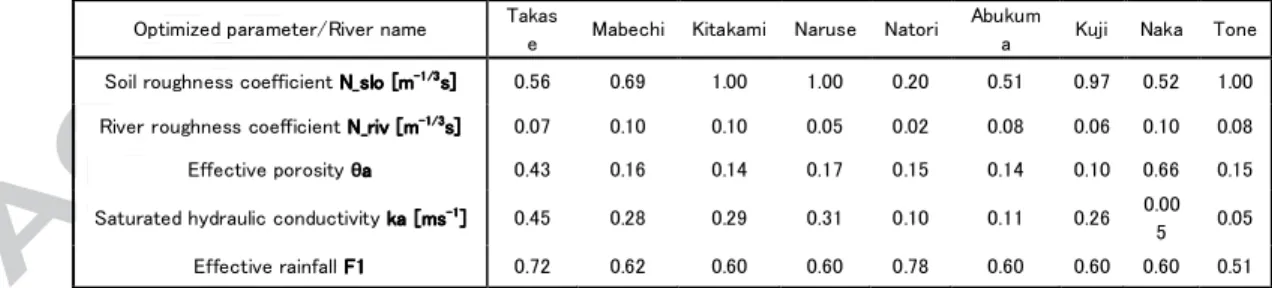
Tables 2 and 3 show optimized parameter values for each of the nine targeted rivers for Typhoon Roke case and Typhoon Chataan case, respectively.
Table 2 Optimized parameter values for each of nine targeted rivers for Typhoon Roke case
Optimized parameter/River name Takas
e Mabechi Kitakami Naruse Natori Abukum
a Kuji Naka Tone Soil roughness coefficient N_slo [mN_slo [mN_slo [mN_slo [m---1/3-1/31/31/3s] s]s]s] 0.56 0.69 1.00 1.00 0.20 0.51 0.97 0.52 1.00
River roughness coefficient N_riv [mN_riv [mN_riv [mN_riv [m----1/31/31/31/3s] s]s]s] 0.07 0.10 0.10 0.05 0.02 0.08 0.06 0.10 0.08
Effective porosity θaaaa 0.43 0.16 0.14 0.17 0.15 0.14 0.10 0.66 0.15 Saturated hydraulic conductivity ka [mska [mska [mska [ms----1111]]]] 0.45 0.28 0.29 0.31 0.10 0.11 0.26 0.00
5 0.05 Effective rainfall F1F1F1F1 0.72 0.62 0.60 0.60 0.78 0.60 0.60 0.60 0.51
Table 3 Optimized parameter values for each of nine targeted rivers for Typhoon Chataan case
Optimized parameter/River name Takas
e Mabechi Kitakami Naruse Natori Abukum
a Kuji Naka Tone Soil roughness coefficient N_slo [mN_slo [mN_slo [mN_slo [m---1/3-1/31/31/3s] s]s]s] 0.36 0.11 1.00 1.00 0.10 1.00 0.27 0.10 1.00
River roughness coefficient N_riv [mN_riv [mN_riv [mN_riv [m----1/31/31/31/3s] s]s]s] 0.03 0.03 0.08 0.06 0.02 0.06 0.08 0.06 0.07
Effective porosity θaaaa 0.27 0.47 0.20 0.10 0.23 0.11 0.11 0.55 0.20 Saturated hydraulic conductivity ka [mska [mska [mska [ms----1111]]]] 0.48 0.40 0.10 0.48 0.50 0.26 0.49 0.50 0.07
Effective rainfall F1F1F1F1 0.63 0.60 0.86 0.68 0.70 0.66 0.60 0.60 0.57
We used SCE-UA optimization method for calibrating different combinations of five parameters. The SCE-UA method can produce similar final results of freshwater outflow to river mouths even if parameters are significantly different, which is described as equifinality issue in calibration of hydrologic models (Beven, 2006). For example, change in both N_slo and ka can influence velocity values and change in both F1 and θa can influence runoff values.
We can see that parameters sometimes change significantly. This is because every river basin has different topographic and geographic characteristics and each typhoon itself has different characteristics, such as path or intensity. These differences may be further amplified because optimized extreme discharge events are the most uncertain events in terms of their physical processes. Using the above described hydrological cell distributed model and parameters optimized for Roke Typhoon rainfalls (calibration), we tested the model applicability for Typhoon Chataan (cross-validation) and vice versa. The results show that Typhoon Chataan validation with calibrated parameters from Typhoon Roke shows higher NS efficiency values than Typhoon Roke validation with calibrated parameters from Typhoon Chataan except for Tone and the rivers located in the northernmost part of the study area, Mabechi and Takase. These results correspond with trajectory paths of two typhoons (Figure 1), because Typhoon Roke’s trajectory was passing directly over Naka, Kuji, and Abukuma basins and in the vicinity of Natori, Naruse, and Kitakami basins. While Typhoon Chataan’s trajectory was passing through the eastern side from Typhoon Roke’s path until it came to the western side on Latitudes closer to Mabechi and Takase Rivers. For the Tone River, in both considered cases, the typhoon trajectory was passing over the river basin and both validation cases have high NS efficiency values (0.915 for Roke validation and 0.837 for Chataan validation). The results suggest that usage of calibrated parameters from the case when a typhoon trajectory passes directly over a river basin may result in higher NS efficiency values when validated with other typhoon cases with similar passage trajectory but further from the river basin.
In subsections 4.1 to 4.3 below, we will show detailed validation results using NS coefficient values for all cases. The results are presented for three largest target rivers: Tone, Kitakami, and
Abukuma as well as results for total outflow from all rivers, while the results for the other six rivers are shown in the Supplementary material. Based on our simulations, freshwater outflow values at the river mouths with and without the effect of the dams included showed to be similar. Therefore, during extreme discharge event the effect of the dam control does not influence freshwater discharge at river mouths significantly, probably because most of dams are located in upstream part of basins.
4.1 Tone River
The case of optimization for Typhoon Roke showed NS = 0.967 for calibration and 0.837 for validation (Typhoon Chataan). The case of optimization for Typhoon Chataan showed NS = 0.920 for calibration and 0.915 for validation (Typhoon Roke). Figure 3a shows calibration results for Typhoon Chataan and Figure 3b shows validation results for Typhoon Roke, while Figure 3c shows calibration results for Typhoon Roke and Figure 3d shows validation results for Typhoon Chataan.
4.2 Kitakami River
As Kitakami River has two mouths, one natural (data from Wabuchi station located west from Oshika peninsula in Ishinomaki city) and one artificial (data from Tome station located north from Oshika peninsula), we optimized parameters with assumption that all water is flowing through the natural river mouth in Ishinomaki city. Later, we divided the total outflow on two parts for the integrated hydrological-oceanographic simulation. We assumed that all water from Tome station is flowing towards the new (artificial) river mouth. Therefore, we used observed discharge from Tome and Wabuchi stations as representative values for the new and old river mouths, respectively. Simulated discharge for the old river mouth was determined from the difference of values between the simulated discharge value at the new river mouth and observed discharge at Tome station for each time step applied for these reanalysis run. The case of optimization for Typhoon Roke showed NS = 0.966 for calibration and 0.813 for validation (Typhoon Chataan). The case of optimization for Typhoon Chataan showed NS = 0.913 for calibration and 0.752 for validation (Typhoon Roke). Figure 4a shows calibration results for Typhoon Chataan. Figure 4b shows validation results for Typhoon Roke. Figure 4c shows calibration results for Typhoon Roke. Figure 4d shows validation results for Typhoon Chataan.
4.3 Abukuma River
The case of optimization for Typhoon Roke showed NS = 0.916 for calibration and 0.710 for validation (Typhoon Chataan). The case of optimization for Typhoon Chataan showed NS = 0.957 for calibration and 0.581 for validation (Typhoon Roke). Figure 5a shows calibration results for Typhoon Chataan. Figure 5b shows validation results for Typhoon Roke. Figure 5c shows calibration results for Typhoon Roke. Figure 5d shows validation results for Typhoon Chataan.
4.4 Total freshwater outflow from all basins
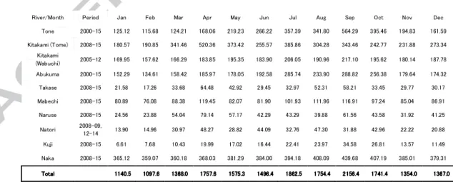
We summarized the total outflow from all river basins in order to simulate the total fresh water budget, flowing from the north-eastern Japanese coast to the western Pacific Ocean during Typhoons Roke and Chataan. The case of optimization for Typhoon Roke showed NS = 0.985 for calibration and 0.858 for validation (Typhoon Chataan). The case of optimization for Typhoon Chataan showed NS = 0.981 for calibration and 0.872 for validation (Typhoon Roke). Figure 6a shows calibration results for Typhoon Roke. Figure 6b shows validation results for Typhoon Chataan. Figure 6c shows calibration results for Typhoon Chataan. Figure 6d shows validation results for Typhoon Roke. Table 4 shows observed monthly mean climatology values for each river separately and for total freshwater outflow from all target rivers.
Table 4 Observed monthly mean climatology values for each river separately and for total freshwater outflow from all targeted rivers (m3/s)
River/Month Period Jan Feb Mar Apr May Jun Jul Aug Sep Oct Nov Dec
Tone 2000-15 125.12 115.68 124.21 168.06 219.23 266.22 357.39 341.80 564.29 395.46 194.83 161.59 Kitakami (Tome) 2008-15 180.57 190.85 341.46 520.36 373.42 255.57 385.86 304.28 343.46 242.77 231.88 273.34
Kitakami
(Wabuchi) 2005-12 169.95 157.62 166.29 183.85 195.35 183.90 206.05 190.96 217.10 195.62 180.14 187.78 Abukuma 2000-15 152.29 134.61 158.42 185.97 178.05 192.58 285.74 233.90 288.82 256.38 179.64 174.32 Takase 2008-15 21.58 17.26 33.68 64.48 42.92 29.45 32.97 52.31 58.21 33.45 29.77 30.17 Mabechi 2008-15 80.89 76.08 88.38 119.45 82.07 81.90 101.93 111.96 116.91 97.24 85.04 86.91 Naruse 2008-15 24.56 23.88 54.04 79.14 57.17 42.29 43.29 39.88 61.56 43.58 31.92 41.25 Natori 2008-09,
12-14 13.90 14.96 30.97 48.27 28.82 44.09 32.76 47.30 31.88 42.96 22.22 20.88 Kuji 2008-15 6.61 7.68 10.43 19.99 17.02 16.44 22.41 23.97 34.58 26.81 13.57 11.49 Naka 2008-15 365.12 359.07 360.18 368.03 381.29 384.00 394.18 408.09 439.68 407.19 385.01 379.31
Total TotalTotal
Total 1140.5 1140.5 1140.5 1140.5 1097.6 1097.6 1097.6 1097.6 1368.0 1368.0 1368.0 1368.0 1757.6 1757.6 1757.6 1757.6 1575.3 1575.3 1575.3 1575.3 1496.4 1496.4 1496.4 1496.4 1862.5 1862.5 1862.5 1862.5 1754.4 1754.4 1754.4 1754.4 2156.4 2156.4 2156.4 2156.4 1741.4 1741.4 1741.4 1741.4 1354.0 1354.0 1354.0 1354.0 1367.0 1367.0 1367.0 1367.0
around 30,000 m3/s while for Typhoon Roke it reached around 23,000 m3/s. For comparison, observed monthly mean climatological discharge for all targeted rivers for July is 1862,5 m3/s and for September is 2156,4 m3/s. The observed climatology discharge for July brings around 5,0·109 m3 of freshwater outflow and single Typhoon Chataan brings to ocean about 5,1·109 m3 of fresh water if consider the peak discharge lasting for 2 days, or more than total expected monthly volume. For the other considered case, the observed climatological discharge in September is expected to be about 5,6·109 m3 and Typhoon Roke gave approximately 4,0·109 m3 of discharge if consider the peak discharge lasting for 2 days, or about 71% from total monthly mean spilled to the ocean.
4.5 Integrated hydrological and oceanographic model
As reference and initial conditions for the described experiments, we used results of 2002 to 2016 reanalysis integration done with JCOPE-T model (Webb et al., 2016). The reanalysis was performed using monthly-mean climatological run-off data for 47 largest Japanese rivers. Two rivers on the Korean Peninsula were also accounted for in the same way. Some rivers, like Tone, which have two estuaries, were treated as two rivers. During the reanalysis integration, every 10 days a model restart point was saved. The nearest restart points, to the beginning of extremal events, were used as initial conditions for sensitivity experiments. Integration was run with hourly river discharges corresponding to the cases under consideration. If hourly discharges were not available, climatological monthly mean values were used. However, it is noteworthy that not all first class Japanese rivers were considered in the ocean reanalysis run. As a result, the reproduced surface salinity distribution in the referenced climatological run and in the initial conditions for sensitivity runs have no persistent local salinity minimum in front of these river mouths. Interestingly, satellite observations show an increased Chl-a concentration in these locations, which may be suggesting that local salinity minimum may be lower than that of our simulations. Based on this experience, future realizations of integrated hydrological and oceanographic model will be considered, including all Japanese first class rivers in the simulations.
Four ocean simulation cases were compared here for each typhoon event. The referenced reanalysis case was carried using climatological mean monthly discharges as freshwater input for the four largest rivers (Tone, Kitakami, Abukuma, Naka), and the other cases using hourly observed and hydrological model simulated discharges estimated by calibration and validation parameters for different
typhoon event, as a real time freshwater input for the nine rivers considered in this study. The simulation cases which included more rivers and hourly realistic freshwater discharges are by no means more reliable. By this comparison, we were trying to estimate deficiency of ocean modeling with climatological discharges used and demonstrate that knowledge of real-time information and hindcasts of extreme river discharges is practically important for correct modeling of coastal processes near river estuaries.
Figure 7a shows initial SSS [PSU], and Figures 7b and 7c show the same distribution 10 days later simulated with observed hourly discharges and climatological monthly mean discharges respectively, for period from July 8, 2002 to July 18, 2002 for the Typhoon Chataan case. Figures 8a-8c show the same results for period September 19, 2011 to 7 days later September 26, 2011 for the Typhoon Roke case. Results from ten days later for Typhoon Chataan case and seven days later for Typhoon Roke case were compared with available daily satellite data which had no coverage in some periods due to important cloud cover associated with typhoon passages.
For the simulation cases with observed discharges, water with low salinity below 31 PSU (blue colors on Figures 7b and 8b), as expected, were formed in front of river estuaries, and were present mostly in Sendai bay as a lens of fresh water for Typhoon Chataan case and extended in a much wider zone and spread much further south along the Japanese Pacific coast, occupying almost the whole coastline between Sendai bay on north and Tone River mouth on south for Typhoon Roke case.
On the north of Honshu Island, low salinity zone (about 3 PSU lower from the initial case for both typhoon events) was generated by Takase and Mabechi Rivers’ extreme discharges. Rivers flowing to the Japan Sea were assumed to provide monthly climatological mean amounts of fresh water and are missing the development of extreme fresher water bodies. Induced ocean circulation in surface layers corresponds to the elevated freshwater’s surface lens formation associated with an intensified river discharges. In the subsurface layers the countercurrent is formed due to the lower pressure associated with the lighter low salinity waters (not shown here). As conclusion, the simulation with observed extreme river discharge is significantly different from the one with climatological mean outflows, and using hydrological model for prediction of real-time extreme river discharges could improve ocean circulation simulation results in coastal areas.
Figures 9a-9d show deviation of SSS [PSU] for integration with hourly observed discharges from that with monthly climatological ones (9a), modeled with calibration parameters minus with
observed data (9b), modeled with validation parameters minus with observed data (9c) and modeled with calibration parameters minus with validation parameters (9d) for the Typhoon Chataan case for July 18, 2002. Figures 9b, 9c and 9d have different (ten times smaller) variations of color scale than Figure 9a. Similarly, Figures 10a-d show the same results for the Typhoon Roke case for 26 September, 2011.
For both Chataan and Roke cases, the impact of accounting hourly discharged reached up to -10 PSU for Typhoon Chataan case and -8 PSU for Typhoon Roke case in Sendai bay, whereas errors from utilization of simulated discharges compared to observed ones do not exceed 2 PSU, with the worst case being when using validation parameters in which case outflow from rivers flowing to the Sendai bay is underestimated compared to observations.
4.6. Validation using remote-sensing data
Salinity observations are quite rare in coastal waters, especially for typhoon weather conditions. Therefore, we used remote-sensing Chl-a concentration as indicator of enhanced river discharge in coastal waters. Specifically, we have compared our modeled results of SSS distribution with available satellite remote-sensing Chl-a concentration data (Sathyendranath et al., 2012). Figure 11 shows 15-Day composites for Chl-a concentration [mgChl/m3] before and 5-Day composites after Typhoon Chataan case. Figure 12 similarly shows 5-Day composites before and after Typhoon Roke case. It should also be mentioned that, due to important cloud cover associated with the typhoon passages, spatial data are missing for most of days, and that only few daily satellite data are used in the calculation of the final composite data.
Observed distributions of increased Chl-a concentration generally correspond well with our decreased SSS modeled results for both typhoon cases. It is noteworthy that modeled reference and associated initial cases for both of the considered typhoons do not account for fresh water discharges from Mabechi and Takase River mouths, while Chl-a satellite data show an increased concentration even for these moderate size rivers. For the Typhoon Chataan case, increased Chl-a and decreased SSS concentrations before the typhoon passage are clearly observed around Tone and Abukuma River mouths, while for Naka and Kitakami River mouths this signal is weaker and less evident likely due to the impact of clouds on the composite satellite Chl-a observation. After the typhoon passage, the largest peaks are
found around Sendai bay as a lens of fresh water and smaller peaks are found alongshore southward from Mabechi and Takase River mouths. The region around Tone River and the Kuroshio front shows no close similarity between observed Chl-a and modeled SSS. This may be caused by strong impact of the Kuroshio Current in modeled ocean circulation in areas close to the current, which could also influence Chl-a concentration locally. For the Typhoon Roke case, increased Chl-a and decreased SSS concentrations before the typhoon are found around Tone, Abukuma, Kitakami and Naka River mouths. After the typhoon passage, the largest peaks are found southward from Sendai bay extending all the way alongshore the coast towards the Kuroshio front, and smaller peaks are found around Mabechi and Takase River mouths.
Several cited studies (Lohrenz et al., 1990, Zheng and Tang, 2007, Hopkins et al. 2013, Racault et al., 2017) have demonstrated that freshwater inflow to oceans and consequent decreased salinity concentrations can be associated with increased Chl-a concentrations, and that the correlation is more conspicuous during extreme discharge events. Our comparison of observed Chl-a and modeled SSS before and after typhoons showed clear correspondence so we used it as the validation method for confirmation of our modeled results.
5 CONCLUSIONS
The extreme discharge events have a lot of uncertainties and differences among their physical processes, but they also have some similarities, which we have focused on in the present study.
For all the nine considered rivers, higher NS efficiency values from two validation cases was always above 0.710 (the lowest being for Abukuma River) and the corresponding calibration case was always above 0.897 (the lowest being for Mabechi River). The calculated NS efficiency values for the total freshwater outflow from all basins were very high, 0.985 for calibration of Typhoon Roke and 0.858 for the same models applied for validation of Typhoon Chataan. Results for Chataan calibration and Roke validation were similar (0.981 and 0.872, respectively).
Evaluation of calibrated and validated NS efficiency values suggest that calibrated parameters for the case when a typhoon trajectory passes directly over a river basin or close to a river basin are more reliable for validation of other typhoons with similar passage trajectory than the other case when calibrated parameters are used from a typhoon with a passage trajectory further away from the river basin.
Even though equifinality was found, i.e., the parameter sets calibrated for the two events were different, cross validation analyses between the two simulation cases gave satisfactory results with respect to the river mouth hydrographs and the SSS response in the coastal zones. These cross validation results suggest that our hydrological models with optimized model parameters calibrated on Typhoon Roke and Chataan cases can be successfully used to predict runoffs values from other extreme precipitation events with similar physical characteristics. This should be confirmed further in future works, by testing the applicability of using this method with many other extreme typhoon event cases in order to obtain a flood forecasting analysis, so that our calibrated hydrological models can be used as nowcasting models for real-time prediction of extreme flooding events.
The effect of dams for the rivers Abukuma, Kitakami, and Tone is shown to be minor because dams are usually built upstream of the basins (not shown).
The model used in the present study has the capability of simulating extreme discharge events through calibration using extreme typhoon case events. The proper simulation of extreme discharge events can be used to improve coastal and ocean modeling, especially in cases that deal with salinity distribution in coastal zones, as demonstrated by the integrated simulation with an ocean model in Section 4.5 (Figures 7, 8, 9 and 10).
Fresh water propagation patterns are different for the two considered cases of extreme event discharges. In the case of Typhoon Chataan, coastal fresh water lenses spread relatively far offshore from Sendai bay, while in the case of Typhoon Roke fresh waters are spreading mainly southward along the Japanese coast with the coastal sea current. There is a significant difference in modeled SSS for the two cases of typhoons impacting Japan, reaching 10 PSU for the Typhoon Chataan case and 8 PSU for the Typhoon Roke case, if hourly observed discharges are used in simulations instead of climatological values. If hourly modeled discharges are used instead of observed ones, both for calibration and validation cases of two events, relative errors are of order no more than 20-25% (2PSU) from the relative difference (8-10 PSU) if hourly observed discharges are used in simulations instead of climatological values. Modeled SSS results were verified by comparison with observed Chl-a concentration reproduced from satellite remote sensing. The decreased SSS results corresponded well with increased Chl-a concentration throughout the entire domain both before and after typhoons passed, with the only one exception being in the Kuroshio front area after the Typhoon Chataan where increased Chl-a
concentration was observed but our model results did not show decreased SSS.
For two simulated typhoon events using two sets of calibrated and validated parameters as well as observation discharge datasets, we get similar results for SSS regardless of which dataset we use, demonstrating the appropriate practical stability of the river models used.
Since most land-ocean combined simulations focus on averaged discharge rather than extreme discharge, our results highlight the importance of incorporating extreme discharges that affect coastal environments in the aftermath of extreme events, which may potentially impact not only on the Chl-a concentration but also the fishery industry.
By having the ability to simulate extreme discharge events at river mouths, this study can be extended to sediment and water quality modeling in coastal areas.
Appendix A. Supplementary material
ACKNOWLEDGEMENTS
This study was supported by the Monbukagakusho (MEXT) scholarship and the Kyoto University Global COE program "Human Security Engineering for Asian Megacities" which were funding the Ph.D. degree study of the first author, who also deeply thanks to The Social Implementation Program on Climate Change Adaptation Technology (SI-CAT) for recent operational and financial support. Corresponding author (Y. Yamashiki) and co-author (T. Sasaki) deeply thanks to Professor Hoshin Gupta at University of Arizona for his support in learning SCE-UA method combining into hydrological model. M-F Racault was supported by the Japan Society for the Promotion of Science (JSPS) Invitational Fellowship for Research in Japan (Long-term) based upon the invitation of Japanese host Prof. Yamagata. The authors would also like to acknowledge the Ocean Colour Climate Change Initiative dataset, Version 3.1, European Space Agency, available online at http://www.esa-oceancolour-cci.org/. The authors are grateful to Adrean Webb and Cassandra Wardinsky for providing English proofread of the manuscript. Finally, we thank to the Associate Editor and two anonymous Reviewers for their useful comments that greatly improved quality of the paper.
Apip, Sayama T, Tachikawa Y, Takara K. 2011. Spatial lumping of a distributed rainfall-sediment-runoff model and its effective lumping scale, Hydrological Processes 26, pp. 855-871. DOI: 10.1002/hyp.8300.
Beven K. 2006. A manifesto for the equifinality thesis, Journal of Hydrology320, pp. 18-36. DOI: 10.1016/j.jhydrol.2005.07.007.
Brando VE, Braga F, Zaggia L, Giardino C, Bresciani M, Matta E, Bellafiore D, Ferrarin C, Maicu F, Benetazzo A, Bonaldo D, Falcieri FM, Coluccelli A, Russo A, Carniel S. 2015. High-resolution satellite turbidity and sea surface temperature observations of river plume interactions during a significant flood event, Ocean Science11, pp. 909-920. DOI: 10.5194/os-11-909-2015.
Carniel S, Warner JC, Chiggiato J, Sclavo M. 2009. Investigating the impact of surface wave breaking on modeling the trajectories of drifters in the northern Adriatic Sea during a wind-storm event, Ocean Modeling30, pp. 225-239. DOI: 10.1016/j.ocemod.2009.07.001.
Carton JA. 1991. Effect of seasonal surface freshwater flux on sea surface temperature in the tropical Atlantic Ocean, Journal of Geophysical Research 96, No. C7, pp. 12593-12598. DOI: 10.1029/91JC01256.
Dai A, Qian T, Trenberth KE, Milliman JD. 2009. Changes in continental freshwater discharge from 1948-2004, Journal of Climate 22, pp. 2773–2792. DOI: 10.1175/2008JCLI2592.1.
Dai A, Trenberth KE. 2002. Estimates of freshwater discharge from continents: latitudinal and seasonal variations, Journal of Hydrometeorology 3, pp. 660-687. DOI: 10.1175/1525-7541(2002)003<0660:EOFDFC>2.0.CO;2.
Dai A, Trenberth KE. 2003. New estimates of continental discharge and oceanic freshwater transport, AMS symposium on observing and understanding the variability of water in weather and climate. Duan Q, Sorooshian S, Gupta VK. 1992. Effective and Efficient Global Optimization for Conceptual Rainfall-Runoff Models, Water Resources Research28, pp. 1015-1031. DOI: 10.1029/91WR02985. Duan Q, Sorooshian S, Gupta VK. 1994. Optimal use of the SCE-UA global optimization method for calibrating watershed models, Journal of Hydrology 158, pp. 265-284. DOI: 10.1016/0022-1694(94)90057-4.
ESRI, ArcGIS Desktop: Release 10.2.2. Redlands, CA: Environmental Systems Research Institute, 2016
Falcieri FM, Benetazzo A, Sclavo M, Russo A, Carniel S. 2014. Po River plume pattern variability investigated from model data, Continental Shelf Research87, pp. 84-95. DOI: 10.1016/j.csr.2013.11.001. Falloon PD, Betts RA. 2006. The impact of climate change on global river flow in HadGEMI simulations, Atmospheric Science Letters7, pp. 62-68. DOI: 10.1002/asl.133.
Fekete BM, Vorosmarty CJ, Grabs W. 2002. High-resolution fields of global runoff combining observed river discharge and simulated water balances, Global Biogeochemical Cycles16, pp. 15-1--15-10. DOI: 15-1--15-10.1029/1999GB001254.
Harada M, Mori M, Tasai H, Hiramatsu K. 2006. Evaluation of Characteristics of TOPMODEL Parameters using SCE-UA Method, Science Bulletin of the Faculty of Agriculture, Kyushu University 61(2), pp. 261-272. (In Japanese)
Hopkins J, Lucas M, Dufau C, Sutton M, Stum J, Lauret O, Channelliere C. 2013. Detection and variability of the Congo River plume from satellite derived sea surface temperature, salinity, ocean colour and sea level, Remote sensing of Environment139, pp. 365-385. DOI: 10.1016/j.rse.2013.08.015.
Hydrosheds: hydrosheds.cr.usgs.gov/index.php. Last access: June 13, 2017
IBTrACKS: www.atms.unca.edu/ibtracs/ibtracs_v03r07/browse-ibtracs/index.php?name=v03r07-2002178N04155. Last access: July 7, 2017
JMA: data.jma.go.jp/risk/obsdl/index.php#. Last access: June 13, 2017
Kida S, Yamashiki Y. 2015. A layered model approach for simulating high river discharge events from land to the ocean. Journal of Oceanography71, pp. 125-132. DOI: 10.1007/s10872-014-0254-4. Knowles N. 2002. Natural and management influences on freshwater inflows and salinity in the San Francisco Estuary at monthly to interannual scales, Water Resources Research 38(12), 1289. DOI: 10.1029/2001WR000360.
Kojima T, Takara K, Oka T, Chitose T. 1998. Resolution influence on the flood runoff analysis result of raster spatial information, Water Engineering Papers42, pp.157-162. (In Japanese)
Lohrenz SE, Dagg MJ, Whitledge TE. 1990. Enhanced primary production at the plume/oceanic interface of the Mississippi River, Continental Shelf Research 10, No. 7., pp. 639-664. DOI: 10.1016/0278-4343(90)90043-L.
Luo P, He B, Takara K, Razafindrabe BHN, Nover D, Yamashiki Y. 2011. Spatiotemporal tend analysis of recent river water quality conditions in Japan, Journal of Environmental Monitoring 13, pp.
2819-2829. DOI: 10.1039/C1EM10339C.
Luo P, Takara K, Apip, He B, Nover D. 2014. Palaeoflood simulation of the Kamo River basin using a grid-cell distributed rainfall run-off model, Journal of Flood Risk Management7(2), pp. 182-192. DOI: 10.1111/jfr3.12038.
Miller JR, Russel GL, Caliri G. 1994. Continental-scale river flow in climate models, Journal of Climate 7, pp. 914-928. DOI: 10.1175/1520-0442(1994)007<0914:CSRFIC>2.0.CO;2.
Milliman JD, Farnsworth KL, Jones PD, Xu KH, Smith LC. 2008. Climatic and anthropogenic factors affecting river discharge to the global ocean, 1951-2000, Global and Planetary Change 62(3-4), pp. 187-194. DOI: 10.1016/j.gloplacha.2008.03.001.
MLIT: www1.river.go.jp. Last access: June 13, 2017
Pratama MA, Yoneda M, Shimada Y, Matsui Y, Yamashiki Y. 2015. Future projection of radiocesium flux to the ocean from the largest river impacted by Fukushima Daiichi Nuclear Power Plant, Scientific Reports (Nature Publishing Group),5: 8408. DOI: 10.1038/srep08408.
Nash JE, Sutcliffe JV. 1970. River flow forecasting through conceptual models part1- a discussion of principles, Journal of Hydrology 10(3), pp. 282-290. DOI: 10.1016/0022-1694(70)90255-6.
NRL: www.nrlmry.navy.mil/tcdat/tc11/WPAC/18W.ROKE/trackfile.txt. Last access: July 7, 2017 Racault MF, Sathyendranath S, Platt T. 2014. Impact of missing data on the estimation of ecological indicators from satellite ocean-colour time-series, Remote Sensing of Environment 152, pp. 15-28. DOI:10.1016/j.rse.2014.05.016.
Racault MF, Sathyendranath S, Brevin RJW, Raitsos DE, Jackson T, Platt T. 2017. Impact of El Nino variability on Oceanic Phytoplankton, Frontiers in Marine Science 4:133. DOI: 10.3389/fmars.2017.00133.
Saha S, Moorthi S, Wu X, Wang J, Nadiga S, Tripp P, Behringer D, Hou Y, Chuang H, Iredell M, Ek M, Meng J, Yang R, Mendez MP, van den Doll H, Zhang Q, Wang W, Chen M, Becker E. 2014. The NCEP Climate Forecast System Version 2, Journal of Climate27, pp. 2185-2208. DOI: 10.1175/JCLI-D-12-00823.1.
Sasaki T. 2014. A study on the method for analysis of radioactive cesium amount of Abukuma basin by distributed runoff model, Master's Thesis of Kyoto University Graduate School of Engineering. (In Japanese)
Sathyendranath S, Brewin B, Müeller D, Doerffer R, Krasemann H, Mélin F, Brockmann C, Fomferra N, Peters M, Grant M, Steinmetz F, Deschamps PY, Swinton J, Smyth T, Werdell J, Franz B, Maritorena S, Devred E, Lee ZP, Hu C, Regner P. 2012. Ocean Colour Climate Change Initiative: Approach and Initial Results, IGARSS 2012, pp. 2024-2027. DOI: 10.1109/IGARSS.2012.6350979.
Sayama T and McDonell JJ. 2009. A new time-space accounting scheme to predict stream water residence time and hydrograph source components at the watershed scale, Water Resources Research45, W07401. DOI: 10.1029/2008WR007549.
Sayama T, Takara K, Tachikawa Y. 2003. Reliability evaluation of rainfall-sediment-runoff-models. IAHS Publications279, pp. 131-141.
Shiklomanov IA. 2009. River runoff to oceans and lakes, Hydrological Cycle 2.
Soeyanto E, Guo X, Ono J, Miyazawa Y. 2014. Interannual variations of Kuroshio transport in the East China Sea and its relation to Pacific Decadal Oscillation and mesoscale eddies, Journal of Geophysical Research: Oceans119, pp. 3595-3616. DOI: 10.1002/2013JC009529.
Sorooshian S, Duan Q, Gupta VK. 1993. Calibration of rainfall-runoff models: Application of global optimization to the Sacramento Soil Moisture Accounting Model, Water Resources Research 29, pp. 1185-1194. DOI: 10.1029/92WR02617.
Tachikawa Y, Nagatani G, Takara K. 2004. The development of the flow-rate relationship formula introducing the mechanism of the saturated or unsaturated flow, Water Engineering Papers 48, pp. 7-12. (In Japanese)
Talley LD. 2002. Salinity patterns in the ocean, Encyclopedia of Global Environmental Change1, pp. 629-640.
Urakawa LS, Kurogi M, Yoshimura K, Hasumi H. 2015. Modeling low salinity waters along the coast around Japan using a high-resolution river discharge dataset, Journal of Oceanography71, pp. 715-739. DOI: 10.1007/s10872-015-0314-4.
Varlamov SM, Guo X, Miyama T, Ichikawa K, Waseda T, Miyazawa Y. 2015. M2 baroclinic tide variability modulated by the ocean circulation south of Japan, Journal of Geophysical Research120(5), pp. 3681-3710. DOI: 10.1002/2015JC010739.
Webb A, Waseda T, Fujimoto W, Horiuchi K, Kiyomatsu K, Matsuda K, Miyazawa Y, Varlamov S, Yoshikawa J. 2016. A High-Resolution, Wave and Current Resource Assessment of Japan: The Web GIS
Dataset. Conference proceedings for AWTEC 2016, pp. 1-6 (arXiv:1607.02251 <https://arxiv.org/abs/1607.02251> [physics.ao-ph]).
Yamashiki Y, Onda Y, Smith HG, Blake WH, Wakahara T, Igarashi Y, Matsuura Y, Yoshimura K. 2014. Initial flux of sediment-associated radiocesium to the ocean from the largest river impacted by Fukushima Daiichi Nuclear Power Plant, Scientific Reports (Nature Publishing Group) 4: 3714. DOI:10.1038/srep03714.
Zheng GM, Tang DL. 2007. Offshore and nearshore chlorophyll increases induced by typhoon winds and subsequent terrestrial rainwater runoff, Marine Ecology Progress Series333, pp. 61–74. DOI: 10.3354/meps333061
Figure 1 Map of the 9 first class Japanese river basins flowing to the western Pacific Ocean and passage tracks (every 6 hours) of typhoons Chataan (red) and Roke (yellow) (ESRI, 2016, IBTrACKS, 2017, NRL, 2017)
Figure 2 Model definition data for Abukuma River. a) Delineated Flow Accumulation data with position of rainfall stations (blue), corresponding Thiessen polygons and observation station Iwanuma (red); b) Delineated Digital Elevation Model; c) Delineated Flow Direction map
Figure 3 Calibration and validation results for Tone River (typhoons Chataan and Roke) Figure 4 Calibration and validation results for Kitakami River (typhoons Chataan and Roke) Figure 5 Calibration and validation results for Abukuma River (typhoons Chataan and Roke)
Figure 6 Calibration and validation results for total freshwater outflow from all basins (typhoons Chataan and Roke)
Figure 7 Initial surface salinity distribution [PSU] (7a), and simulated 10 days later with observed hourly discharges (7b) and climatological monthly mean discharges (7c) for period from July 8, 2011 to July 18, 2011 for the typhoon Chataan case
Figure 8 Initial surface salinity distribution [PSU] (8a), and simulated 7 days later with observed hourly discharges (8b) and climatological monthly mean discharges (8c) for period from September 19, 2011 to September 26, 2011 for the typhoon Roke case
Figure 9 Deviation of surface salinity [PSU] for integration with hourly observed discharges from that with monthly climatological ones (9a), modeled with calibration parameters minus with observed data (9b), modeled with validation parameters minus with observed data (9c) and modeled with calibration parameters minus with validation parameters (9d) for the typhoon Chataan case for July 18, 2002
Figure 10 Deviation of surface salinity [PSU] for integration with hourly observed discharges from that with monthly climatological ones (10a), modeled with calibration parameters minus with observed data (10b), modeled with validation parameters minus with observed data (10c) and modeled with calibration parameters minus with validation parameters (10d) for the typhoon Roke case for September 26, 2011 Figure 11 15-Day composites for Chlorophyll-a concentration [mgChl/m3] before typhoon (left) and 5-Day composites after typhoon Chataan (right)
Figure 12 5-Day composites for Chlorophyll-a concentration [mgChl/m3] before typhoon (left) and after typhoon Roke (right)
(a)
(b)
(a) (b)
(a) (b)
(a) (b)
(a) (b)
(a) Initial (b) Observed (c) Climatological
(a) Initial (b) Observed (c) Climatological
(a) Obs - Clim (b) Cal - Obs (c) Val - Obs (d) Cal - Val
(a) Obs - Clim (b) Cal - Obs (c) Val - Obs (d) Cal - Val
HIGHLIGHTS
Hourly simulated extreme freshwater outflows were integrated with JCOPE-T ocean model
Projection of coastal Sea Surface Salinity (SSS) was improved with freshwater input
Decreased SSS results corresponded well with increased observed Chl-a concentrations
Extreme freshwater outflows significantly affect SSS distribution in the coastal zone