The Simple Concurrent Online Processing System (SCOPS) - an open-source interface for remotely sensed data processing
M.A. Warren a, S. Goult a, D. Clewley a
a Plymouth Marine Laboratory, Plymouth, PL1 3DH, UK
Corresponding author: Mark Warren - [email protected]
Abstract
Advances in technology allow remotely sensed data to be acquired with increasingly higher spatial and spectral resolutions. These data may then be used to influence government decision making and solve a number of research and application driven questions. However, such large volumes of data can be difficult to handle on a single personal computer or on older machines with slower components. Often the software required to process data is varied and can be highly technical and too advanced for the novice user to fully understand. This paper describes an open-source tool, the Simple Concurrent Online Processing System (SCOPS), which forms part of an airborne hyperspectral data processing chain that allows users accessing the tool over a web interface to submit jobs and process data remotely. It is demonstrated using Natural Environment Research Council Airborne Research Facility (NERC-ARF) instruments together with other free- and open-source tools to take radiometrically corrected data from sensor geometry into geocorrected form and to generate simple or complex band ratio products. The final processed data products are acquired via an HTTP download. SCOPS can cut data processing times and introduce complex processing software to novice users by distributing jobs across a network using a simple to use web interface.
1 2 3
4
5
6
7
8 9 10 11 12 13 14 15 16 17 18 19 20 21 22 23
1. Introduction
Remote sensing is a technique that can produce a large amount of data very quickly and is often used to collect data over large areas where it would be too time consuming or hazardous to collect the data via in situ methods. A typical hyperspectral remote sensing instrument acquires information in the form of data-cubes: a 3-dimensional array with two spatial dimensions and a third spectral dimension. This third dimension together with the instrument field of view and spatial resolution means that even a modest survey can result in a large volume of data. These data are often many gigabytes (GB) in size and processing can be time consuming and require significant processing resources. For example, the Specim AISA Fenix (http://www.specim.fi/products/aisafenix-hyperspectral-sensor/) instrument can acquire data from up to 622 spectral bands, where a 10 minute acquisition (equating to a flight line distance of 80 km) could easily generate a 7 GB raw data file. A typical airborne hyperspectral survey could consist of 10 - 20 flight lines of this size (each in a separate file) resulting in greater than 100 GB of raw data.
There are two main problems associated with processing such datasets: i) the availability of specialised software with which to process data, and ii) the computational resources to carry out processing. A data processing and archive facility (PAF) can easily handle these volumes but end-users (e.g. university researchers, students) may have restricted computational power available.
Remote sensing PAFs often provide a data portal or web interface to allow users to search for and order data, for example the space agencies ESA (https://earth.esa.int/web/guest/data-access), NASA (https://earthdata.nasa.gov/earth-observation-data/near-real-time/download-nrt-data) and JAXA (https://www.gportal.jaxa.jp). More recently, third party open-source data portals and processors have been designed such as the THREDDS Data Server (Unidata, 25
26 27 28 29 30 31 32 33 34 35 36 37 38
39 40 41 42 43
44 45 46 47 48
2016), GISportal (https://github.com/pmlrsg/GISportal) and RasDaMan (Baumann et al., 1998) that allow individuals to host portals that provide remote data access with the ability to process data via an internet browser. The co-location of data storage and processing facilities has seen an increase in recent years, and with the rise in volume of freely available data it is beneficial to be able to serve only the data that researchers want rather than have them download data they do not need. In the UK, the JASMIN (http://www.jasmin.ac.uk/) facility has become available to the UK and European climate and Earth-system science communities. JASMIN is described as a “data-cluster” and is a combination of a super-computer and data-centre, providing storage and hosted cloud computing (Lawrence et al., 2013).
A proof of concept for processing EO data on distributed systems was performed by Petcu et al. (2010) for education and training purposes. Other tools such as CATENA (Krauss et al., 2013), operated at the German Aerospace Center (DLR), is an automatic end-to-end optical processing system for satellite data, which uses a reference image to generate ground control points to orthorectify the data. SEPAL (https://github.com/openforis/sepal), an open source cloud-based data analysis processor, is a software package that allows users to access Sentinel and Landsat imagery for land monitoring purposes. However, the authors are not aware of a distributed processing system for airborne hyperspectral data, aimed specifically for end users of the data.
In this study we have created an open-source tool that allows a distributed (internet-based) processing chain for airborne hyperspectral data acquired by SPECIM push-broom sensors. It can be set up on any suitable webserver or workstation and allows data processing jobs to be defined and submitted to a compute node via a Python back-end. It is written in an extendable fashion such that adaptations can be easily made. It provides a simple interface to airborne 49
50 51 52 53 54 55 56 57 58
59 60 61 62 63 64 65 66 67
68 69 70 71 72
specialised computer knowledge or equipment. It has the ability for remote deployment so that data processing can be submitted on a single machine but performed on a separate machine or machines. Other open- and free-source tools are employed in the following demonstration to provide a chain that can perform band ratio-ing and geocorrection of hyperspectral data. Note that the difference between “free source” and “open source” is that the source code is available but restrictions on usage prevent it being defined as open source.
For an out-of-the-box experience, SCOPS is set up integrated with the Airborne Processing Library (APL, Warren et al. (2014)) software for geocorrection of SPECIM airborne sensors. An instance of this is set up on the JASMIN facility and integrated with the Natural Environment Research Council Airborne Research Facility (NERC-ARF) dataset for UK-based researchers to use. Currently the archive of NERC-ARF data contains SPECIM hyperspectral data dating from 2006 to 2017 inclusive acquired by Eagle, Hawk, Fenix and Owl instruments.
This manuscript is ordered such that section 2 gives an overview of the requirements for general airborne hyperspectral processing, section 3 contains a description of the tool, including both front and back ends and the integration with other free-source tools. Section 4 details the external software packages that are required to run SCOPS. Section 5 describes case studies where the tool is deployed: (a) at Plymouth Marine Laboratory (PML) and (b) on the JASMIN system. Further case studies demonstrate the basic usage of SCOPS, the update of SCOPS for the inclusion of a new module and an atmospheric correction module. A discussion with conclusions is presented in section 6.
2. Airborne hyperspectral processing 74
75 76 77 78 79
80 81 82 83 84 85 86
87 88 89 90 91 92 93 94
95
It is prudent to introduce here the aspects of hyperspectral data processing that are typically required after survey, but also to distinguish between those tasks usually performed by the PAF and those by the end user. Processing of airborne hyperspectral data usually requires at least three stages performed by the PAF: navigation data processing and synchronisation, calibration and geocorrection. Further processing stages such as atmospheric correction are vital, especially for comparing to other data sets, for example ground spectra or data acquired on a different date. This may be performed by the PAF or left as a task to the user.
Navigation data processing and synchronisation is the process of taking GPS and Inertial Measurement Unit (IMU) data from the plane, alongside surveyed positions of instruments and look angle. From these data the position of the instruments and where they are pointing at regular time intervals for the duration of each flight line is determined. Calibration is required to convert the digital numbers recorded by the sensor into relevant SI units and correct for noise terms (e.g. see Ahern et al. (1987), Cocks et al. (1998)). Geocorrection converts the data from instrument geometry into physical or map geometry using a regime of resampling and interpolation (Toutin (2004), Schläpfer and Richter (2002), Müller et al. (2002)). As part of the geocorrection process a digital elevation model (DEM) is used to correct for distortions due to surface topography. Once the navigation processing and calibration have been carried out by the PAF, most researchers are unlikely to require repeating these steps.
Although most researchers ultimately want to work with geocorrected data, it is often beneficial to apply algorithms to the data prior to the geocorrection stage, for example to avoid artefacts from interpolation or when instrument geometry is preferred. Often researchers would like to apply their own algorithms rather than use an algorithm applied by a PAF and will do the processing themselves from the calibrated data and map the derived product. When geocorrecting data there are a number of options for which researchers are 97
98 99 100 101 102 103
104 105 106 107 108 109 110 111 112 113 114
115 116 117 118 119 120
likely to want to select for themselves such as output projection, interpolation algorithm and pixel size. Many of these choices are application specific.
The geocorrection stage takes substantial computational effort. For example, using the Airborne Processing Library to geocorrect a calibrated Fenix flight line of 2.9 GB takes an old laptop computer running Fedora 22, with 1 GB RAM and an Intel Core Duo T2400 @ 1.83 GHz processor 76 minutes. The resulting file size, mapped at 4 m pixel size, is 22 GB. On a more modern PC running Fedora 21 with 16GB RAM and an Intel i5-3550 CPU @ 3.3 GHz processor, the same file took 9 minutes. As well as (and linked to) the increase in available RAM, disk IO will play a substantial part in this time difference with modern solid state drives offering improved performance over traditional disks. For the majority of researchers the machines available to them are likely to fall somewhere between these two extremes.
Another consideration with airborne data is that unlike satellite remote sensing, where a single scene can be sufficient to cover a study site, multiple flight lines are normally required from airborne surveys. This adds to the computational requirements in that, not only is the processing intensive, it must be repeated for all lines within a flight. Repetition of the same process multiple times makes batch processing particularly important.
3. Simple Concurrent Online Processing System
The Simple Concurrent Online Processing System (SCOPS) has been developed to aid end-user’s processing of large remote sensing data sets on cluster / grid style computers. The drive behind this is to enable people with low-end computer resources to get the most out of the data. The current setup of SCOPS is being demonstrated for processing airborne 121
122
123 124 125 126 127 128 129 130 131 132
133 134 135 136 137
138
139
140 141 142 143
hyperspectral data, using the APL software, but could equally be used for satellite data or other data – it would simply just mean replacing components of the Python code and updating appropriately. Case studies in section 5 demonstrate the extension of SCOPS to add a new processing module and to include an atmospheric correction module.
Typically the PAF will have radiometrically and geometrically calibrated the data, fixed any issues arising from the navigation data and delivered the data in a consistently formatted package. In this manuscript we focus on the current usage of SCOPS for end-users who have data that have already been calibrated. However, it would be possible to update SCOPS to work from the raw data but this would require technical knowledge about the sensors, dealing with navigation file formats and unforeseen problems that can occur at data collection (e.g. missing metadata, sensor malfunctions), and is therefore a task for the PAF rather the end-user.
The APL software has been developed by the UK NERC-ARF for processing hyperspectral data from SPECIM sensors, including the AISA Eagle, Hawk, Fenix and Owl instruments. For details on the geocorrection algorithms see Warren et al. (2014). An out-of-the-box experience with SCOPS links with APL to process NERC-ARF data from these sensors.
SCOPS is comprised of two parts: an internet facing front-end and Python back-end. These interact via a system of status flags and cron jobs. The rationale behind keeping these separate is two-fold: security and performance. Intensive processing should not be done on the web server as this will cause the performance of any other services, including web sites, to reduce. The security benefit comes from the fact that the back-end scripts ‘pull’ the requests from the front-end, rather than the front-end ‘pushing’ them. This means that if the security of the webserver is compromised the data servers and processing nodes remain secure.
144 145 146 147
148 149 150 151 152 153 154 155
156 157 158 159
160 161 162 163 164 165 166 167
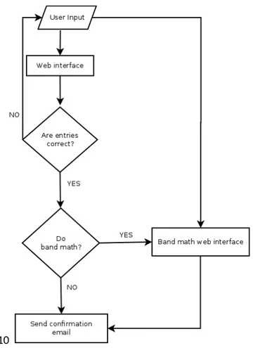
A description of each of the parts follows with flow diagrams of the processes shown in Figures 1 and 2.
3.1 Front-end
The frontward facing part of the tool is constructed from HTML templates, javascript and a Python flask web application run through a web server gateway interface. A configuration file is used to control the parameters that an operator may wish to change depending on the environment the code is running in. This includes input data locations and output locations as well as administrative details such as the email address used to contact users. The input data needs to be relevant for the processing software used by the back-end. In this implementation APL is used as the data processing tool, and the input data should be the NERC-ARF data delivery directory. This contains the radiometrically calibrated sensor data, synchronised navigation data and sensor view vector files required by APL. When the front-end page loads it checks these data are all present.
There are two main pages that the user interacts with: the project page and the band ratio page. The project page controls the resampling and gridding of the hyperspectral data based on the user inputs. This page is populated with information based on data from either a directory structure or a database. The user is prompted to enter their email address (which in usual setup is required for authentication of the request but can be turned off via the config file) and then has to make the following choices. There is an option to select geographic projection (British National Grid, Universal Transverse Mercator or the option to define a projection via a PROJ4 string). There is an option to upload a digital elevation model or to use one automatically generated from SRTM or ASTER DEM data. The image resampling interpolation method can be selected from nearest-neighbour, bilinear or cubic spline. There 168
169
170
171
172 173 174 175 176 177 178 179 180 181
182 183 184 185 186 187 188 189 190 191
are options to define the pixel size of the output gridded data, the region to be processed (whole flight line or a region of interest) and which bands of which products to geocorrect. Initially these inputs are set to the optimal values based on a generic user (e.g. pixel size based on aircraft altitude and sensor field-of-view). Some basic checking of the user entered parameters is performed – such as the pixel size being a numeric value, the region of interest contains data and the PROJ4 string is accepted by the PROJ4 library – and any problems found are highlighted for the user to fix.
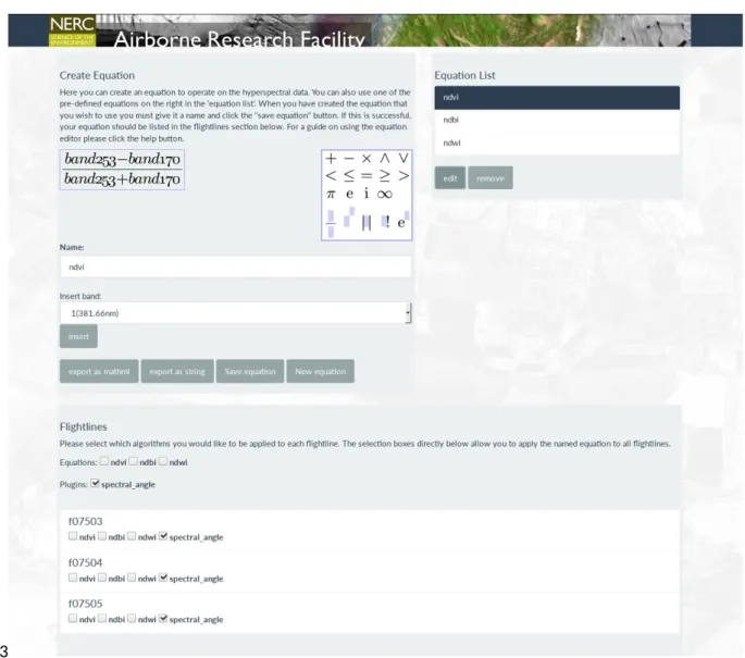
The band ratio page is shown only if the user requested it from the project page. Here the user can insert equations using MathML or select an equation from the supplied list (normalised difference vegetation index (Metternicht, 2003), normalised difference built-up index (Zha et al., 2003), normalised difference water index (Gao, 1996)) and specify them to be run on any or all of the data. Currently the only supported operations are band math functions. The equations are converted to javascript functions and checked that they result in a numeric value. If they fail then the user is prompted to correct the equation before continuing. The user is now also able to select any available plugins to run on the data.
At the submission of this page the user will be prompted to check for new email and click the link within it. This will set the status of the job to confirmed and allow the back-end to start processing.
192 193 194 195 196 197 198
199 200 201 202 203 204 205 206
207 208 209
Figure 1: Flow diagram of the front-end operation.
3.2 Back-end
After the user has submitted the processing a configuration file is created. This lists all the flight lines that are to be processed and the various options that the user specified, including any post-processing band ratio formulae to be run. The configuration file is then picked up by the Python back-end scripts via a crontab.
The back-end scripts are designed to be completely separate from the web interface. They perform the task of processing the data, preparing for delivery (compressing the deliverables) and monitoring the progress of the operation.
210
211
212 213
214 215 216 217
218 219 220
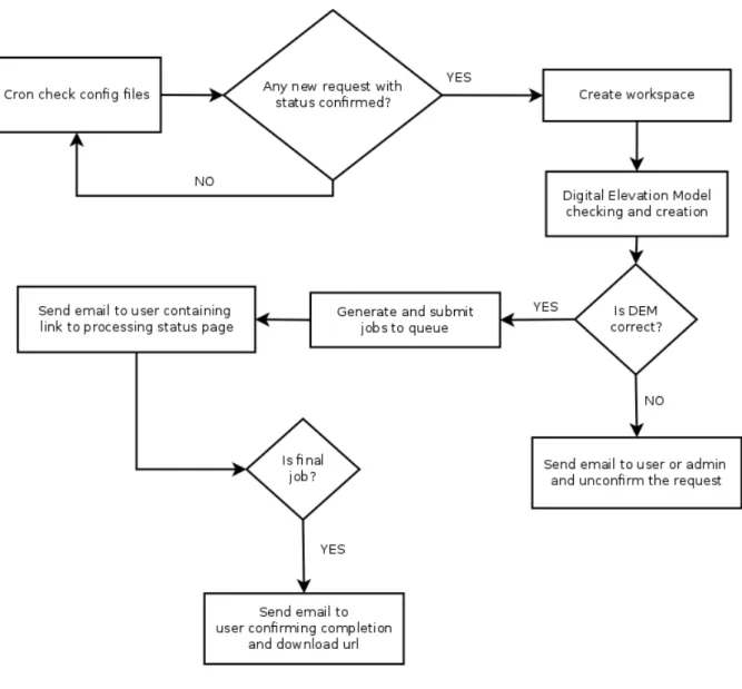
The flow of the processing is shown in Figure 2. A cron job runs every 10 minutes and checks the configuration files in the configuration workspace for the status keywords. If it finds one whose status is confirmed but not submitted then it will generate a new workspace for the processing of this request. It will also either check the user uploaded DEM is in the required format (a raster file which can be read using the Geospatial Data Abstraction Library; GDAL) and that it covers the entire region being processed, or generate a new one if no DEM was uploaded. If the DEM check fails then it will email the user a message stating this, or if the DEM generation fails then it will email the system administrator and pause operation until manual intervention to fix the error state.
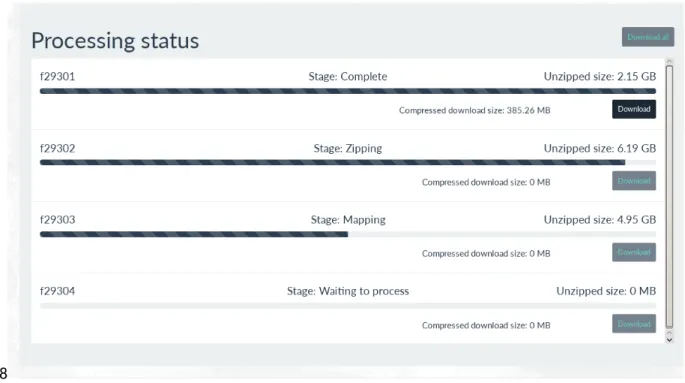
Once the DEM has been generated or confirmed to be correct, the individual jobs are created and submitted for processing. At this point an email is sent to the user containing a link to the status web page (see Figure 3). This page shows dynamic progress bars for each job so that the user is kept informed of the processing status. Submission of jobs is controlled by the job scheduling system used by the back-end scripts. Each job, when it finishes, checks to see if it is the final one processing. If it is, then it will archive all the processed data into a single file and email the user with a link to the final compressed archive file for download. The user is also able to download the individual compressed flight lines from the status page.
221 222 223 224 225 226 227 228 229
230 231 232 233 234 235 236 237
Figure 2: Flow diagram of the back-end operation.
The software is designed to be easily modified for different processing environments. A configuration file is used to keep track of the environment variables, parameters and executables. Different command line driven software can be operated from the back-end by updating the process_command script. Indeed, it is possible to have multiple process_command scripts with each one set up to use different geocorrection software, allowing the expansion of SCOPS to cover multiple operations. SCOPS can also pause jobs and resume on different queues. This is useful to run software on specific machines, or to allow one job to wait until another has finished before continuing.
238
239
240 241 242 243 244 245 246 247
Figure 3: Progress status page. This shows the progress of each job, the size of the
compressed and uncompressed data, and gives the user the option to download individual files as and when they are completed.
3.3 Extensions
Extensions to the processing chain are relatively easy to implement. An example of this is the option to perform band ing of the hyperspectral data. If the user selects the band ratio-ing radio button before submittratio-ing the request, they are redirected to the band ratio-ratio-ing web interface. This allows the user to select pre-defined equations such as normalised difference vegetation index (NDVI) or to build their own equation using the equation editor.
After submission the back-end sorts the jobs to separate the standard georeferencing ones from the band ratio-ing, with each type of job being sent to a different process_command. The band ratio-ing is built and performed using Python libraries. For more extensive 248
249 250 251
252
253
254 255 256 257 258
259 260 261
operations, a third party package such as the open source RasDaMan raster manipulation software (Baumann et al., 1998) could be easily incorporated into the processing chain.
To add new extensions, there is a plugins directory (whose path can be set in the configuration file) where users can add standalone Python scripts to do further processing. There are two things required when adding a new module. The first is that the module must contain a function named “run” that does all the processing and returns a string file path of the output filename. The second is to edit the line_handler function in the scops_process_apl_line.py file to add any keyword arguments into the plugin_args dictionary. The SCOPS front-end will automatically pick up any python file in the plugins directory and add checkboxes to the per-line processing list on the bandmaths page, labelled by the name of the module. The back-end will then run the modules that have been selected by the user, by looping through each of the selected plugin run functions.
4. Dependency packages
As previously mentioned, additional software packages are required to operate with SCOPS. The front-end runs as a flask application (http://flask.pocoo.org/) on the server. It employs the MathDox javascript library (Cohen et al., 2003) to enable the equation design on the band ratio and uses javascript for checks on the user input before submitting the web form.
For the back-end, it is assumed the standard Python distribution is installed together with the following packages: GDAL, PROJ, SQLite, numpy and numexpr. SCOPS uses the open source digital elevation model generation package NERC-ARF DEM Scripts (Clewley et al., 2017) to generate a DEM for the region when users do not upload their own. This requires access to elevation data such as the global ASTER elevation product 262
263
264 265 266 267 268 269 270 271 272 273
274
275
276 277 278 279
280 281 282 283 284
(https://asterweb.jpl.nasa.gov/gdem.asp) or SRTM elevation product (http://www2.jpl.nasa.gov/srtm/), both of which are available to freely download. The free source APL package is used to geocorrect and generate resampled images from the data.
These tools have been chosen because they are all free to use for not-for-profit applications and their source code is available which allows one to edit the software’s interface if required.
5. Case studies
To demonstrate SCOPS a few case studies have been created. The first gives an overview of user operation of SCOPS. The second demonstrates SCOPS implemented on two different systems where the back-end has been employed on a multi-machine grid at Plymouth Marine Laboratory (PML), UK and the JASMIN super-cluster located at Harwell, UK. The front-end was only installed at PML on a virtual machine running CentOS 7. This was used to generate configuration files for both tests. The third and fourth case studies show how to extend SCOPS by adding new modules: a spectral angle classifier and an atmospheric correction module.
5.1 Step by step procedural usage of SCOPS
This case study demonstrates the procedure of using SCOPS from a user perspective. The front-end page is shown in Figure 4. The user will enter their email address, select which lines and bands they wish to process, whether to mask out pixels, set up the output grid projection, pixel size, resampling method and select the DEM to use for the geocorrection. 285
286 287
288 289 290
291
292
293 294 295 296 297 298 299 300
301
302
303 304 305 306
text input occurs with the pixel size and region of interest definition. This makes the checking of user input trivial. Here they also have the option to perform some band maths on the files. If selected, SCOPS will present the user with the page shown in Figure 5. On this page the user can select from pre-prepared formulae (NDVI, NDWI, NDBI) or enter a new one. Also any plugins (see section 5.3) will be listed here. Whilst the data is being processed the user can get information on the status and download individual lines when they become available from the webpage (Figure 3).
308 309 310 311 312 313 314
17 316
Figure 4: The front-end web portal of SCOPS as employed at PML. (Top) shows the selection of flight lines and bands to process; (Bottom) shows the other options such as masking, DEM selection, projection and grid definition.
Figure 5: The band math page of SCOPS. Band math equations can be constructed using the equation builder, saved or selected from the equation list and exported. Equations and plugin modules can be run on a per-flight-line basis using the checkboxes near the bottom of the page.
318 319 320
321 322
323 324 325 326 327
5.2 A demonstration on two processing environments 5.2.1 PML grid
The multi-node grid based at PML consists of 150 compute nodes and 4 masters. The nodes are of varying specification ranging from older models with 8 GB RAM and Intel Xeon 3075 CPUs @ 2.6 GHz to more modern ones with 64 GB RAM and Intel Xeon E5-2637 CPUs @ 3.5 GHz. The number of jobs that can run per node is a function of the RAM reserved for that job and the number of cores on the node. The number of cores ranges from 4 to 8. The nodes are each connected to switches with 1 gigabit connections whereas the file servers are connected to switches with 10 gigabit connections. Each node used in this test was running Fedora 21. The grid is managed by the Open Grid Scheduler software, where individual jobs are dispatched for serial batch processing using qsub.
5.2.2 JASMIN
The JASMIN infrastructure currently comprises around 4000 cores over multiple nodes. System RAM ranges from 4GB per core up to hosts with 512GB. Each node has a 10 gigabit connection to a 40 gigabit core network. The nodes used for this test were running Red Hat Enterprise Linux Server version 6.8. The grid is managed using the IBM Load Sharing Facility (LSF) with jobs dispatched for serial processing using bsub. More information can be found from the JASMIN website (http://www.jasmin.ac.uk/).
5.2.3 Results
A dataset consisting of 52 flight lines acquired from a Specim AisaFenix hyperspectral sensor 329
330
331 332 333 334 335 336 337 338 339
340
341
342 343 344 345 346 347
348
349
basic NDVI was selected from the band ratio-ing window. On the PML system the final email to download the zip archive of processed data arrived 277 minutes after initial submission with 21 different grid nodes in total being used, although only 3 were used at any one time. This is so as not to cause bottlenecks with too many read / write requests hitting the file server at the same time. The final zip archive file size was 40 GB but data were also available as individual zip files per flight line as and when they became available.
Running the same processing on the JASMIN infrastructure the time from job submission to finishing zipping the final archive was 22 minutes. Due to the availability of a faster file system all jobs were allowed to run at once rather than imposing a limit.
5.3 Adding an extension
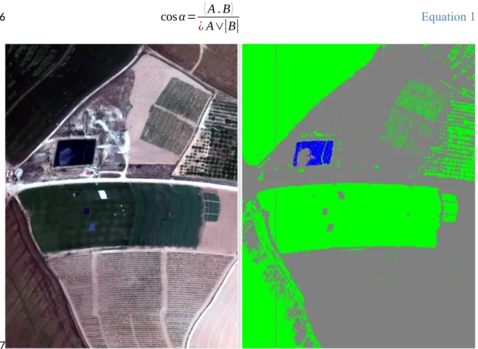
Here a module to add a spectral angle classifier (Kruse et al., 1993) is used to demonstrate the process of adding an extension. The spectral angle classifier module reads in an ASCII reference spectra file which contains delimited columns for wavelength and spectra. Here the spectra classes used are vegetation, mineral and water, and have been previously extracted from the data file itself. If a spectral library or field data collected from the survey site are available then they can be used as the reference spectra (just replace the ref_spectra.txt file). The angle between each reference spectra and each image pixel is calculated using the dot product, equation 1, where A and B are the reference and image pixel spectra vectors.
The reference spectra that produces the smallest angle, and therefore most similar in spectral shape, is selected as the class for that particular pixel. The output is a file with a single band of integer numbers denoting class for each pixel (Figure 6). This is a fairly simple and rudimentary classification but serves as an example for extending SCOPS with a new module.
352 353 354 355 356 357
358 359 360
361 362
363 364 365 366 367 368 369 370
371 372 373 374 375
cosα=
⟨
A . B⟩
¿A∨|B| Equation 1
Figure 6. (Left) the original hyperspectral image; (Right) the classification of the image, where different colours denote the different classes (blue = water, grey = mineral, green = vegetation). The vertical grey line in the classification is the result of an unmasked bad pixel.
5.4 Atmospheric correction
Atmospheric correction is vital when comparing data from different sensors or dates. SCOPS has a module for atmospheric correction built upon the ATCOR-4 software (Richter and Schläpfer, 2002). As ATCOR-4 is not an open licenced software package this module is not provided with SCOPS, but the same principles would apply to a module built upon another package such as 6S (Vermote et al., 1997).
376
377 378 379 380
381
382
383 384 385 386 387
The atmospheric correction method using ATCOR-4 is based on the method outlined in (Markelin et al., 2017), with parameters for the atmospheric correction such as water vapour and aerosol optical thickness automatically derived such that minimal manual intervention is required. Within SCOPS the atmospheric correction stage runs between the masking of level1b data and mapping stage.
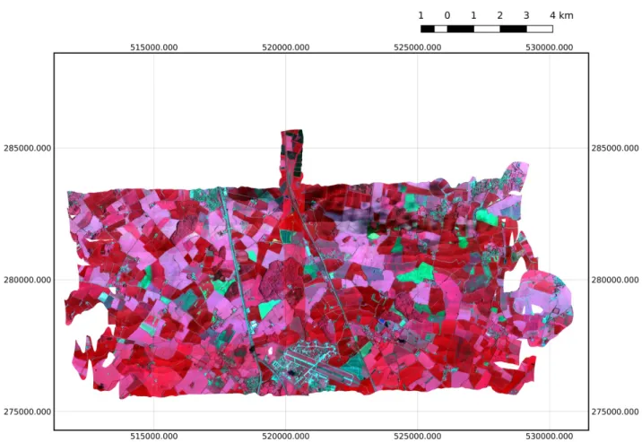
To demonstrate the atmospheric correction module, data over Monks Wood, Cambridge, UK acquired in June 2014 were used. The purpose was to derive a series of narrow-band hyperspectral indices relating to leaf chemistry, water content and health which will be combined with other data (e.g., LiDAR) to examine bird species distributions. To ensure indices calculated are consistent across all lines it is important to apply atmospheric correction first. Figure 7 shows the atmospherically corrected data that would then be used to derive the hyperspectral indices from.
388 389 390 391 392
393 394 395 396 397 398 399
Figure 7. False colour VNIR composite of the atmospherically corrected data over Monks Wood, UK, made from 17 flight lines. Note areas of cloud shadow present in the North East.
6. Discussion
SCOPS is a web-based distributed processing system for hyperspectral data and has been created using open- and free-source software. It gives people with low computing resources, for example developing nations or students, a simple and easy to use interface to access data processing capabilities. SCOPS has been used to handle the initial user request, submit jobs and inform the user of the progress and email final download links for the data. Using the system on the JASMIN infrastructure allowed 54 lines from a single flight to be processed in 22 minutes compared to 618 minutes when using a single CPU. More importantly, it allows the user to keep the resource heavy process off their machine, allowing them to continue with 400
401 402 403 404
405 406 407 408 409 410 411 412
other tasks or power off their machine. SCOPS can also be installed and operated on a single computer or over an internal network rather than the internet. This could be done, for example, to employ a simple user interface to what otherwise could be very complex command-line driven software.
Airborne hyperspectral data have been used to demonstrate the procedure, but SCOPS could quite easily be used for other data sources too (e.g. satellite data products). The tool has been designed to allow easy modular insertions of new or different tools into the processing chain as demonstrated using a spectral angle mapper. The use of configuration files to set parameters such as data directories and software binaries allows easy updates without needing to change the core code. SCOPS is in the process of being set up as a service to allow researchers who use the UK NERC-ARF to process their data via a web interface. The source code is available to download from GitHub at the following addresses:
Frontend: https://github.com/pmlrsg/SCOPS_frontend
Backend: https://github.com/pmlrsg/SCOPS_processing
The development of SCOPS raised some unexpected issues. Initially a status flag method was used to monitor the job progression but was later updated to use a SQLite database to store the processing status. This is more extendable, cleaner and a secure way to monitor the status that doesn’t involve the access of filesystems across different servers or through firewalls. Another important lesson learnt was that data delivery (download of large files) can still be an issue across slow networks. This led to the per-flight-line zipped downloads rather than the whole dataset. The implementation of SCOPS on JASMIN is hoped to mitigate this for UK researchers as further analysis can be performed on the JASMIN system before data download. A push towards cloud-based Earth Observation analysis systems such as SEPAL is envisioned.
413 414 415 416
417 418 419 420 421 422 423 424
425
426
427 428 429 430 431 432 433 434 435 436
The implementation of SCOPS on two systems (PML and JASMIN) with differing hardware and queue submission systems has given some insight into difficulties that can arise and the use of configuration files tries to mitigate changing code when running on different systems (e.g. using variables to store executable names). However, inevitably some alterations will be required for new systems. A final lesson has been learnt from listening to user feedback and trying to understand the difficulties faced with command-line driven batch processing versus a user-friendly web interface. This has led to a simple design to allow access to users who may otherwise be discouraged from using airborne hyperspectral data.
Acknowledgements
The data used in this study were acquired and provided by the U.K Natural Environment Research Council Airborne Research Facility (NERC-ARF) and are available from the Centre for Environmental Data Analysis (CEDA): http://www.ceda.ac.uk/. This work has been developed as part of the NERC-ARF Data Analysis Node.
References
Ahern, F.J., Brown, R.J., Cihlar, J., Gauthier, R., Murphy, J., Neville, R.A., Teillet, P.M., 1987. Review article: Radiometric correction of visible and infrared remote sensing data at the canada centre for remote sensing. International Journal of Remote Sensing 8, 1349-1376, 10.1080/01431168708954779.
Baumann, P., Dehmel, A., Furtado, P., Ritsch, R., Widmann, N., 1998. The multidimensional database system RasDaMan. SIGMOD Rec. 27, 575-577, 10.1145/276305.276386. 437
438 439 440 441 442 443 444
445
446
447 448 449 450
451
452
453 454 455 456 457 458
Clewley, D., Goult, S., Warren, M., 2017. NERC-ARF DEM Scripts 0.2.2. Zenodo, 10.5281/zenodo.322341.svg.
Cocks, T., Jenssen, R., Stewart, A., Wilson, I., Shields, T., 1998. The Hymap airborne hyperspectral sensor: the system, calibration and performance, 1st EARSEL Workshop on Imaging Spectroscopy, Zurich.
Cohen, A.M., Cuypers, H., Barreiro, E.R., Sterk, H., 2003. Interactive mathematical documents on the web, In Algebra, Geometry and Software Systems. Springer-Verlag, pp. 289-306.
Gao, B.-c., 1996. NDWI—A normalized difference water index for remote sensing of vegetation liquid water from space. Remote Sensing of Environment 58, 257-266, 10.1016/S0034-4257(96)00067-3.
Krauss, T., d'Angelo, P., Schneider, M., Gstaiger, V., 2013. The Fully Automatic Optical Processing System Catena at DLR. ISPRS - International Archives of the
Photogrammetry, Remote Sensing and Spatial Information Sciences, 177-183, 10.5194/isprsarchives-XL-1-W1-177-2013.
Kruse, F.A., Lefkoff, A.B., Boardman, J.W., Heidebrecht, K.B., Shapiro, A.T., Barloon, P.J., Goetz, A.F.H., 1993. The spectral image processing system (SIPS)—interactive visualization and analysis of imaging spectrometer data. Remote Sensing of Environment 44, 145-163, 10.1016/0034-4257(93)90013-N.
Lawrence, B.N., Bennett, V.L., Churchill, J., Juckes, M., Kershaw, P., Pascoe, S., Pepler, S., Priitchard, M., Stephens, A., 2013. Storing and manipulating environmental big data with JASMIN, IEEE Big Data, San Francisco, 10.1109/BigData.2013.6691556. Markelin, L., Simis, S., Hunter, P., Spyrakos, E., Tyler, A., Clewley, D., Groom, S., 2017.
Atmospheric Correction Performance of Hyperspectral Airborne Imagery over a 459
460 461 462 463 464 465 466 467 468 469 470 471 472 473 474 475 476 477 478 479 480 481 482
Small Eutrophic Lake under Changing Cloud Cover. Remote Sensing 9, 2-22, 10.3390/rs9010002.
Metternicht, G., 2003. Vegetation indices derived from high-resolution airborne videography for precision crop management. International Journal of Remote Sensing 24, 2855-2877, 10.1080/01431160210163074.
Müller, R., Lehner, M., Müller, R., Reinartz, P., Schroeder, M., Vollmer, B., 2002. A program for direct georeferencing of airborne and spaceborne line scanner images, ISPRS, Commission I, WG I/5., pp. 1-3.
Petcu, D., Panica, S., Neagul, M., Frincu, M., Zaharie, D., 2010. Earth observation data processing in distributed systems. Informatica 34, 463-476.
Richter, R., Schläpfer, D., 2002. Geo-atmospheric processing of airborne imaging
spectrometry data. Part 2: Atmospheric/topographic correction. International Journal of Remote Sensing 23, 2631-2649, 10.1080/01431160110115834.
Schläpfer, D., Richter, R., 2002. Geo-atmospheric processing of airborne imaging spectrometry data - Part 1: parametric orthorectification. International Journal of Remote Sensing 23, 2631-2649.
Toutin, T., 2004. Review article: Geometric processing of remote sensing images: models, algorithms and methods. International Journal of Remote Sensing 25, 1893-1924, 10.1080/0143116031000101611.
Unidata, 2016. THREDDS Data Server (TDS) version 4.6.2. UCAR/Unidata, Boulder, CO, 10.5065/D6N014KG.
Vermote, E.F., Tanre, D., Deuze, J.L., Herman, M., Morcette, J.J., 1997. Second Simulation of the Satellite Signal in the Solar Spectrum, 6S: an overview. IEEE Transactions on Geoscience and Remote Sensing 35, 675-686, 10.1109/36.581987.
483 484 485 486 487 488 489 490 491 492 493 494 495 496 497 498 499 500 501 502 503 504 505 506
Warren, M.A., Taylor, B.H., Grant, M.G., Shutler, J.D., 2014. Data processing of remotely sensed airborne hyperspectral data using the Airborne Processing Library (APL): Geocorrection algorithm descriptions and spatial accuracy assessment. Computers & Geosciences 64, 24-34, 10.1016/j.cageo.2013.11.006.
Zha, Y., Gao, J., Ni, S., 2003. Use of normalized difference built-up index in automatically mapping urban areas from TM imagery. International Journal of Remote Sensing 24, 583-594, 10.1080/01431160304987.
507 508 509 510 511 512 513
514