Artificial Neurons with Arbitrarily
Complex Internal Structures
G.A. Kohring
C&C Research Laboratories, NEC Europe Ltd.
Rathausallee 10, D-53757 St. Augustin, Germany
Abstract
Artificial neurons with arbitrarily complex internal structure are intro-duced. The neurons can be described in terms of a set of internal variables, a set activation functions which describe the time evolution of these variables and a set of characteristic functions which control how the neurons interact with one another. The information capacity of attractor networks composed of these generalized neurons is shown to reach the maximum allowed bound. A simple example taken from the domain of pattern recognition demon-strates the increased computational power of these neurons. Furthermore, a specific class of generalized neurons gives rise to a simple transformation relating attractor networks of generalized neurons to standard three layer feed-forward networks. Given this correspondence, we conjecture that the maximum information capacity of a three layer feed-forward network is 2 bits per weight.
Keywords: artificial neuron, internal structure, multi-state neuron, attractor
net-work, basins of attraction
1
Introduction
The typical artificial neuron used in neural network research today has its roots in the McCulloch-Pitts [15] neuron. It has a simple internal structure consisting of a single variable, representing the neuron’s state, a set of weights representing the the input connections from other neurons and an activation function, which changes the neuron’s state. Typically, the activation function depends upon a sum of the product of the weights with the state variable of the connecting neurons and has a sigmoidal shape, although Gaussian and Mexican Hat functions have also been used. In other words, standard artificial neurons implement a simplified version of the sum-and-fire neuron introduced by Cajal [22] in the last century.
Contrast this for a moment to the situation in biological systems, where the functional relationship between the neuron spiking rate and the membrane mem-brane potential is not so simple, depending as it does on a host of neuron specific parameters [22]. Furthermore, even the notion of a typical neuron is suspect, since mammalian brains consists of many different neuron types, many of whose functional role in cognitive processing is not well understood.
In spite of these counter examples from biology, the standard neuron has pro-vided a very powerful framework for studying information processing in artificial neural networks. Indeed, given the success of current models such as those of Little-Hopfield [14, 8], Kohonen [12] or Rumelhart, Hinton and Williams [20], it might be questioned whether or not the internal complexity of the neuron plays any significant role in information processing. In other words, is there any press-ing reason to go beyond the simple McCulloch-Pitts neuron?
This paper examines this question by considering neurons of arbitrary internal complexity. Previous researchers have attempted to study the affects of increasing neuron complexity by adding biologically relevant parameters, such as a refrac-tion period or time delays, to the neuro-dynamics (see e.g. Clark et al., 1985). The problem with such investigations is that they have so far failed to answer the question of whether such parameters are simply an artifact of the biological nature of the neuron or whether the parameters are really needed for higher-order infor-mation processing. To date networks with more realistic neurons look more bio-logically plausible, but their processing power is not better than simpler networks. An additional problem with such studies, is that as more and more parameters are added to the neuro-dynamics, software implementations becomes too slow to allow one to work with large, realistically sized networks. Although using silicon neurons [16] can solve the computational problem, they introduce their own set of artifacts which may add or detract from their processing power.
The approach taken here differs from earlier work by extending the neuron while keeping the neuro-dynamics simple and tractable. In doing so, we will be able to generalize the notion of the neuron as a processing unit, thereby moving
beyond the biological neuron to include a wider variety of information process-ing units. (One has to keep in mind, that the ultimate goal of the artificial neural network program is not to simply replicate the human brain, but to uncover the general principles of cognitive processing, so as to perform it more efficiently than humans are capable of.) As a byproduct of this approach, we will demonstrate a formal correspondence between attractor networks composed of generalized arti-ficial neurons and the common three layer feed-forward network.
The paper is organized as follows: In the next section, the concept of the gener-alized artificial neuron is introduced and its usefulness in attractor neural networks is demonstrated, whereby the information capacity of such networks is calculated. Section three presents a simple numerical comparison between networks of gener-alized artificial neurons and the conventional multi-state Hopfield model. Section four discusses various forms that the generalized artificial neuron can take and the meaning to be attached to them. Section five discusses generalized generalized neurons with interacting variables. The paper ends with a discussion on the merits of the present approach. Proofs and derivations are relegated to the appendix.
2
Generalized Artificial Neurons (GAN)
Since its introduction in 1943 by McCulloch and Pitts, the artificial neuron with a single internal variable (hereafter referred to as the McCulloch-Pitts neuron) has been a standard component of artificial neural networks. The neuron’s internal variable may take on only two values, as in the original McCulloch and Pitts model, or it may take on a continuum of values. Although, even where analog or continuous neurons are used, it is usually a matter of expediency, e.g., learning algorithms such as back-propagation [20] require continuous variables even if the application only makes use of a two state representation.
Whereas the McCulloch-Pitts neuron presupposes that a single variable is suf-ficient to describe the internal state of a neuron, we will generalize this notion by allowing neurons with multiple internal variables. In particular, we will describe the internal state of a neuron byQvariables.
Just as biological neurons have no knowledge of the internal states of other neurons, but only exchange electro-chemical signals (Shepherd, 1983), a gener-alized artificial neuron (GAN) should not be allowed knowledge of the internal states of any other GAN. Instead, each GAN has a set of, C, characteristic
func-tions,f ff i
:R Q
!R ; i=1;:::;Cg, which provide mappings of the internal
variables onto the reals. It is these characteristic functions which are accessible by other GANs. Even though the characteristic functions may superficially resemble the neuron firing rate, no such interpretation need be imposed upon them.
variables of a GAN are described by a deterministic dynamics. Here we distin-guish between the different dynamics of the Qinternal variables by defining Q
activation functions, A
i. These activation functions may depend only upon the
values returned by the characteristic functions of the other neurons.
A GAN,N(Q;f;A), is thus described by a a set of internal variables,Q, a set
of activation functions,A, and set of characteristic functions,f. Note, for the case
of McCulloch-Pitts neuron, there is only a single internal variable governed by single activation function taking on one of two values: 0or1, which also doubles
as the characteristic function.
Now, to combine these neurons together into a network, we must define a net-work topology. The topology is usually described by a set of numbers, fW
ij g
(i;j = 1;:::;N), called variously by the names couplings, weights, connections
or synapses, which define the edges of a graph having the neurons sitting on the nodes. (In this paper we will use the term “weight” to denote these numbers.) Ob-viously, many different network topologies are definable, each possessing its own properties, therefore, in order to make some precise statements, let us consider a specific topology, namely that of a fully connected attractor network [14, 8]. Attractor networks form a useful starting point because they are mathematically tractable and there is a wealth of information already known about them.
2.1
Attractor Networks
For simplicity, consider the case where each of the Q internal variables is
de-scribed by a single bit, then the most important quantity of interest is the informa-tion capacity per weight,E, defined as:
E
Numberof bitsstored Numberof weights
(1)
For a GAN network the number of weights can not simply be the number of
fW ij
g, otherwise it would be difficult for each internal variable to evolve
indepen-dently. The simplest extension of the standard topology is to allow each internal variable to multiply the weights it uses by an independent factor. Hence, instead of fW
ij
g we effectively havefW a ij
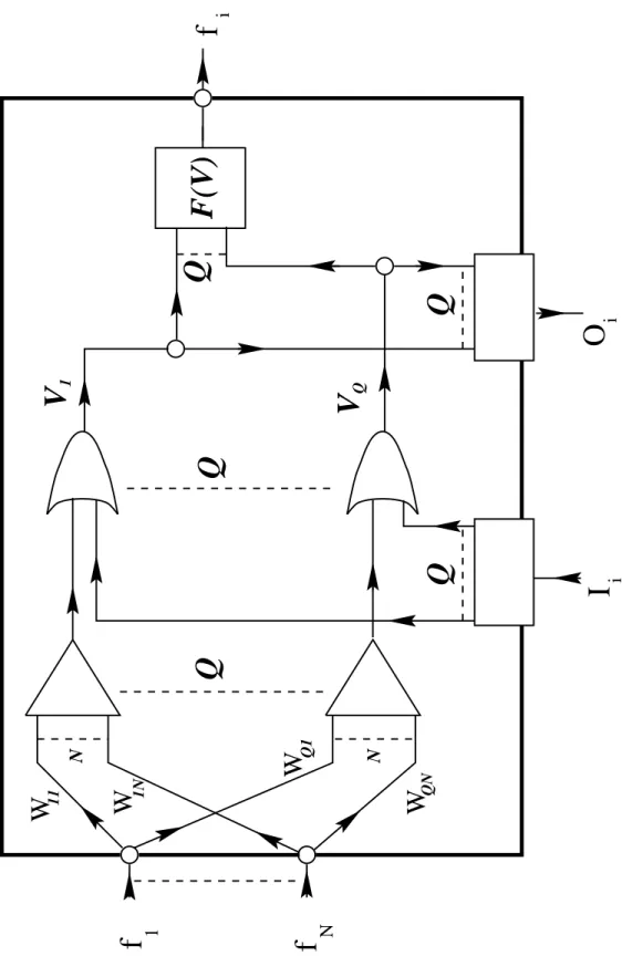
g, where, a = 1;:::;Q. A schematic of this
type of neuron is given in Figure 1. In an attractor network, the goal is to storeP
patterns such that the network functions as an auto-associative, or error-correcting memory. The information capacity,E, for these types of networks is then:
E =
QPN QN
2
= N
bpw; (2)
(bpc bits per weight) As is well known, there is a fundamental limit on the
information capacity for attractor networks, namely E 2 bpw [1, 4, 13, 17].
This implies,P 2N.
Can this limit be reached with a GAN? To answer this question, consider the case where the activation functions are simply Heaviside functions,H:
V a i (t+1) = H 0 N X j6=i J a ij I j N (t) 1 A O i N (t+1) = F V 1 i (t+1);:::;V Q i (t+1) (3) whereH(x) = 0ifx < 0andH(x) = 1ifx 0. s a i
(t+1)represents the the a-th internal variable of the i-th neuron. The weight to the internal states of the i-th neuron does not violate the principle stated above, because the i-th neuron
still has no knowledge of the internal states of the other neurons and each neuron is free to adjust its own internal state as it sees fit.
In appendix A we use Gardner’s weight space approach [4] to calculate the information capacity for a network defined by Eq. 3, where we now take into account the fact that the total number of weights has increased fromN
2
toQN 2
. Letdenote the probability thats
a
=0and1 the probability thats a
=1, then E for Eq. 3 becomes:
E = ln 2 (1 )ln 2 (1 ) 1 + 1 2 (2 1)erf (x= p 2) bpw; (4)
wherexis a solution to the following equation:
(2 1) " e x 2 =2 p 2 x 2 erf(x= p 2) # =(1 )x; (5)
anderf (z)is the complimentary error function: erf (z)=(2= p ) R 1 z dye y 2 . When = 1=2, i.e., when s has equal probability of being0 or1, then x = 0 and the information capacity reaches its maximum bound of E = 2 bpw.
For highly correlated patterns, e.g., ! 1, the information capacity decreases
somewhat, E ! 1=(2ln2)bpw, but, more importantly, it is still independent of Q.
What we have shown is that networks of GANs store information as efficiently as networks of McCulloch-Pitts neurons. The difference being, that in the former, each stored pattern containsNQbits of information instead ofN. Note: we have
neglected the number of bits needed to describe the characteristic functions since they are proportional toQN, which for largeN is much smaller than the number
of weights,QN 2
.
3
A Simple Example
Before continuing with our theoretical analysis, let us consider a simple, concrete example of a GAN network that illustrates their advantages over conventional neural networks. Again, we consider an attractor network composed of GANs. Each GAN has two internal bit-variablesQ =fs
1 ;s
2
gwhose activation functions
are given by Eq. 3 and two characteristic functions, f =fg;hg. Letg q 1 q 2 andhq 1 +2q
2. In the neurodynamics defined by Eq. 3 we will use the function g, reserving the function hfor communication outside of the network. (There is
no reason why I/O nodes should use the same characteristic functions as compute nodes.)
The weights will be fixed using a generalized Hebbian rule [6, 8], i.e.,
W a ij = P X =1 s a; i f j (6)
Since this GAN has 4 distinct internal states, we can compare the performance of our GAN network to that of a multi-state Hopfield model [19]. Define the neuron values in the multi-state Hopfield network ass2f 3; 1;1;3gand define
thresholds at f 2;0;2g. (For a detailed discussion regarding the simulation of
multi-state Hopfield models see the work of Stiefvater and M ¨uller [23].)
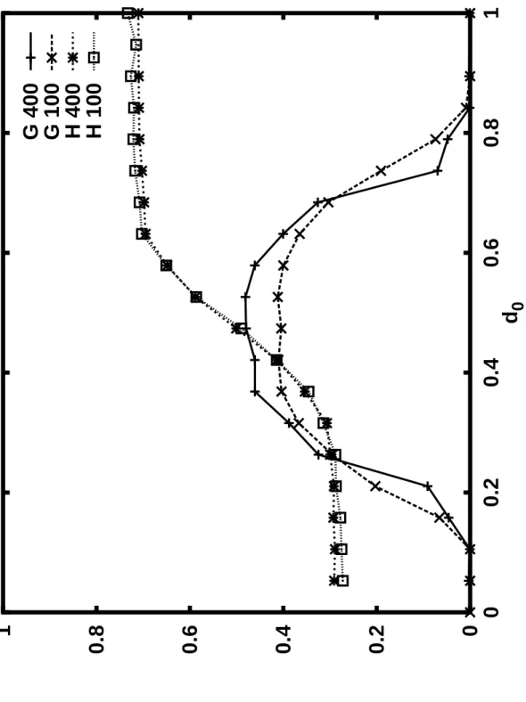
Fig. 2 depicts the basins of attraction for these two different networks, i.e.,d 0
is the initial distance from a given pattern to a randomly chosen starting configu-ration and < d
f
>is the average distance to the same pattern when the network
has reached a fixed point. For both network types, random sets of patterns were used with each set consisting of P = 0:05N patterns. The averaging was done
over all patterns in a given set and over 100 sets of patterns.
There are two immediate differences between the behavior of the multi-state Hopfield network and the present network: 1) the recall behavior is much better for the network of GANs, and 2) using theXORfunction as a characteristic
func-tion when there are an even number of bit variables, results in a mapping between a given state and its anti-state (i.e., the state in which all bits are reversed), for this reason the basins of attraction have a hat-like shape instead of the sigmoidal shape usually seen in the Hopfield model.
This simple example illustrates the difference between networks of conven-tional neurons and networks of GANs. Not only is the retrieval quality improved,
but, depending upon the characteristic function, there is also a qualitative differ-ence in the shape of the basins of attraction.
4
Characteristic Functions
Until now the definition of the characteristic functions,f, has been deliberately left
open in order to allow us to consider any set of functions which map the internal variables onto the reals: f ff :R
Q
!R g. In section 2 no restrictions on the f
were given, however, an examination of the derivation in appendix A, reveals that the characteristic functions do need to satisfy some mild conditions before Eq. 4 holds: 1) jhfij p N; 2) hf 2 iN; and 3) hf 2 i hfi 2 6=0: (7)
The first two conditions are automatically satisfied if f is a so-called squashing
function, i.e,f :R Q
! [0;1℄.
4.1
Linear
fand Three Layer Feed-Forward Networks
One of the simplest forms for f is a simple linear combination of the internal
variables. Let the internal variables, s a i
(t), be bounded to the unit interval, i.e., s a i 2 [0;1℄, and let J a i
denote the coefficients associated with the i-th neuron’s a-th internal variable, thenf becomes:
f i (t)= Q X a=1 J a i s a i (t): (8) Provided, j P Q a=1 J a i j p
N, and provided not all J a i
are zero, the three con-ditions in Eq. 7 will be satisfied. Since the internal variables are bounded to the unit interval, let their respective activation functions be any sigmoidal function,S.
Then we can substituteS into Eq. 8 in order to obtain a time evolution equation
solely in terms of the characteristic functions:
f i (t)= Q X a=1 J a i S 0 N X j6=i W a ij f j (t 1) 1 A : (9)
Formally, this equation is, for a giveni, equivalent to that of a three layer neural
the hidden layer and one linear neuron on the output layer. From the work of Leshno et al.1, we know that three layer networks of this form are sufficient to approximate any continuous function F : R
N 1
! R to any degree of accuracy
provided Qis large enough. Leshno et al.’s result applied to Eq. 9 shows that at
each time step, a network ofN GANs is capable of approximating any continuous
functionF :R N
!R
N
to any degree of accuracy.
In section 2.1 the information capacity of a GAN attractor network was shown to be given by the solution of eqs. 4 and 5. Given the formal correspondence demonstrated above, the information capacity of a conventional three layer neural network must be governed by the same set of equations. Hence, the maximum information capacity in a conventional three layer network is limited to 2 bits per weight.
4.2
Correlation and Grandmother functions
A special case of the linear weighted sum discussed above is presented by the correlation function: f i (t)= 1 Q Q X a=1 t a i s a i (t); (10) where theft a i
grepresent a specific configuration of the internal states ofN(Q;f).
With this form for f, the GANs can represent symbols using the following
inter-pretation for f: as f ! 1, the symbol is present, and as f ! 0 the symbol
is not present. Intermediate values represent the symbols partial presence as in fuzzy logic approaches. In this scheme, a symbol is represented locally, but the information about its presence in a particular pattern is distributed. Unlike other representational schemes, by increasing the number of internal states, a symbol can be represented by itself. Consider, for example, a pattern recognition system. IfQis large enough, one could represent the symbol for a tree by using the
neu-ron firing pattern for a tree. In this way, the symbol representing a pattern is the pattern itself.
Another example forf in the same vein as Eq. 10 is given by:
f i (t)=Æ fs a i (t)g;ft a i g ; (11) where, Æ
x;y is the Kronecker delta function: Æ
x;y
= 1 iff x = y. This equation
states thatf is one when the value of all internal variables are equal to their values
in some predefined configuration. A GAN of this type represents what is some-times called a grandmother cell.
1Leshno et al.’s proof is the most general in a series of such proofs. For earlier, more restrictive
4.3
Other Forms of
fObviously, there are an infinite number of functions one could use forf, some of
which can take us beyond conventional neurons and networks, to a more general view of computation in neural network like settings. Return for a moment to the example discussed in section 3:
f i (t)= Q O a=1 s a i (t): (12)
This simply implements the parity function over all internal variables. Its easy to see that hfi = 1=2and hf
2
i hfi 2
= 1=4, hence, this form off fulfills all the
necessary conditions. Using the XORfunction as a characteristic function for a
GAN trivially solves Minsky and Papert’s objection to neural networks [18] at the expense of using a more complicated neuron.
Of course Eq. 12 can be generalized to represent any Boolean function. In fact, each f
i could be a different Boolean function, in which case the network
would resemble the Kauffman model for genomic systems [11], a model whose chaotic behavior and self-organizational properties have been well studied.
5
Neurons with Interacting Variables
So far we have considered only the case where the internal variables of the GAN are coupled to the characteristic function of other neurons and not to each other, however, in principle, there is no reason why the internal variables should not interact. For simplicity consider once again the case of an attractor network. The easiest method for including the internal variables in the dynamics is to expand Eq. 3 by adding a new set of weights, denoted by,fL
ab i
g, which couple the internal
variables to each other:
s a i (t+1)=H 0 N X j6=i W a ij f j + Q X b6=a L ab i s b i 1 A : (13)
Using the same technique we use in section 2.1, we can determine the new infor-mation capacity for attractor networks (see appendix A):
E =E 0 1+ r (1 ) h 2 i hi 2 2 (1+) 1+ (1 ) h 2 i hi 2 ; (14) where, E 0 is given by Eq. 4,
Q=N andhi is the average value of the
fluc-tuations in the characteristic functions are equal to the flucfluc-tuations in the internal variables, thenE =E
0, otherwise,
Eis always less thanE 0.
6
Summary and Discussion
In summary, we have introduced the concept of the generalized artificial neuron (GAN),N(Q;f;A), whereQis a set of internal variables,f is a set characteristic
functions acting on those variables andAis a set of activation functions
describ-ing the dynamical evolution of those same variables. We then showed that the information capacity of attractor networks composed of such neurons reaches the maximum allowed value of 2 bits per weight. If we use a linear characteristic function `a la Eq. 8, then we find a relationship between three layer feed forward networks and attractor networks of GANs. This relationship tells us that attractor networks of GANs can evaluate an arbitrary function of the formF :R
N
! R
N
at each time step. Hence, their computational power is significantly greater than that of attractor networks with two state neurons.
As an example of the increased computation power of the GAN, we presented a simple attractor network composed of four state neurons. The present network significantly out performed a comparable multi-state Hopfield model. Not only were the quantitative retrieval properties better, but the qualitative features of the basins of attraction were also fundamentally different. It is this promise of ob-taining qualitative improvements over standard models that most sets the GAN approach apart from previous work.
In section 2.1, the upper limit on the information capacity of an attractor net-work composed of GANs was shown to be 2 bits per weight, while, in section 4.1 we demonstrated a formal correspondence between these networks and con-ventional three layer feed-forward networks. Evidently, the information capacity results apply to the more conventional feed-forward network as well.
The network model presented here bears some resemblance to models involv-ing hidden (or latent) variables (see e.g., [7]), however, there is one important difference: namely, the hidden variables in other models are only hidden in the sense that they are isolated from the network’s inputs and outputs; but they are not isolated from each other, they are allowed full participation in the dynamics, including direct interactions with one another. In our model, the internal neural variables interact only indirectly via the neurons’ characteristic functions.
Very recently, Gelenbe and Fourneau [5] proposed a related approach they call the “Multiple Class Random Neural Network Model”. Their model also in-cludes neurons with multiple internal variables, however, they do not distinguish between activation and characteristic functions, furthermore, they restrict the form of the activation function to be a stochastic variation of the usual sum-and-fire rule,
hence, their model is not as general as the one presented here.
In conclusion, the approach advocated here can be used to exceed the limi-tations imposed by the McCulloch-Pitts neuron. By increasing the internal com-plexity we have been able to increase the computational power of the neuron, while at the same time avoiding any unnecessary increase in the complexity of the neuro dynamics, hence, there should be no intrinsic limitations to implementing our generalized artificial neurons.
References
[1] COVER, T. M. Capacity problems for linear machines. In Pattern
Recogni-tion (New York, 1968), L. Kanal, Ed., Thompson Book Company, pp. 929–
965.
[2] EDWARDS, S. F., ANDANDERSON, P. W. Theory of spin glasses. Journal
of Physics F 5 (1975), 965–974.
[3] FUNAHASHI, K. On the approximate realization of continuous mappings by
neural networks. Neural Networks 2 (1989), 183–192.
[4] GARDNER, E. The space of interactions in neural network models. Journal
of Physics A 21 (1988), 275–270.
[5] GELENBE, E.,ANDFOURNEAU, J.-M. Random neural networks with
mut-liple classes of signals. Neural Computation 11 (1999), 953–963.
[6] HEBB, D. O. The Organization of Behavior. John Wiley & Sons, New York,
1949.
[7] HINTON, G. E., ANDSEJNOWSK I, T. J. Learning and Relearning in
Boltz-mann Machines. In Rumelhart et al. [21], 1986, pp. 282–317.
[8] HOPFIELD, J. J. Neural networks and physical systems with emergent col-lective computational abilities. Proceedings of the National Academy of
Sci-ence, USA 79 (1982), 2554–2558.
[9] HORNIK, K. Approximation capabilities of multilayer feed-forward net-works. Neural Networks 4 (1991), 251–257.
[10] HORNIK, K., STINCHCOMBE, M., AND WHITE, H. Multilayer
feedfor-ward networks are universal approximators. Neural Networks 2 (1989), 359– 366.
[11] KAUFFMAN, S. A. Origins of Order: Self-Organization and Selection in
Evolution. Oxford University Press, Oxford, 1992.
[12] KOHONEN, T. Self-Organization and Associative Memory. Springer-Verlag,
Berlin, 1983.
[13] KOHRING, G. A. Neural networks with many-neuron interactions. Journal
[14] LITTLE, W. A. The existence of persistent states in the brain. Mathematical
Bioscience 19 (1974), 101–119.
[15] MCCULLOCH, W. S., AND PITTS, W. A logical calculus of the idea
im-manent in nervous activity. Bulletin of Mathematical Biophysics 5 (1943), 115–133.
[16] MEAD, C. Analog VLSI and Neural Systems. Addison-Wesley, Reading,
1989.
[17] MERTENS, S., K ¨OHLER, H. M.,ANDBOS, S. Learning grey-toned patterns in neural networks. Journal of Physics A 24 (1991), 4941–4952.
[18] MINSKY, M., ANDPAPERT, S. Perceptrons: An Introduction to
Computa-tional Geometry. MIT Press, Cambridge, 1969.
[19] RIEGER, H. A. Storing an extensive number of gray-toned patterns in a
neural network using multi-state neurons. Journal of Physics A 23 (1990), L1273–L1280.
[20] RUMELHART, D. E., HINTON, G. E.,ANDWILLIAMS, R. J. Learning
rep-resentations by error propagation. In Rumelhart et al. [21], 1986, pp. 318–
362.
[21] RUMELHART, D. E., MCCLELLAND, J. L., AND THE PDP RE
-SEARCH GROUP, Eds. Parallel Distributed Processing. MIT Press,
Cam-bridge, MA, 1986.
[22] SHEPHERD, G. M. Neurobiology. Oxford University Press, Oxford, 1983.
[23] STIEFVATER, T., AND M ¨ULLER, K.-R. A finite-size scaling investigation forq-state hopfield models: Storage capacity and basins of attractions.
N N
Q
11W
Q
f
f
W
W
QN Q1W
1Nf
QV
Q
Q
Q
F(V)
i iO
N 1 i 1V
I
Figure 1: A schematic of a generalized artificial neuron. f
i denotes the value
of thei-th neuron’s characteristic function, these are the values communicated to
0
0.2
0.4
0.6
0.8
1
0
0.2
0.4
0.6
0.8
1
<d
f>
d
0G 400
G 100
H 400
H 100
Figure 2: Basins of attraction for a GAN network (lower curves) and for a multi-state Hopfield model (upper curve). In both cases the number of stored patterns is
A
Derivation of the Information Capacity
For simplicity consider a homogeneous network ofN GANs, where theQinternal
variables of each neuron are simply bit-variables. In addition, we will consider the general case of interacting bits. Given P patterns, with
i representing the
characteristic functions and a
i the internal bit-variables, then by equation eqs. 3
and 13, we see that these patterns will be fixed points if:
(2 a i 1) 0 N X j6=i W a ij i + Q X b=1 L ab i b i 1 A >0: (15)
In fact, the more positive the left hand side is, the more stable the fixed points. Using this equation we can write the total volume of weight space available to the network for storingP patterns as:
V = Y i;a V a i ; (16) where, V a i = 1 Z a i Z Y j dW a ij Y b dL ab i Æ 0 N X j6=i (W a ij ) 2 N 1 A Æ 0 Q X b6=a (L ab i ) 2 Q 1 A Y H 2 4 (2 a i 1) 0 1 p N N X j6=i W a ij j + 1 p N Q X b6=a L ab i b i a i 1 A 3 5 ; (17) and Z a i = Z Y j dW a ij Y b dL ab i Æ 0 N X j6=i (W a ij ) 2 N 1 A Æ 0 Q X b6=a (L ab i ) 2 Q 1 A : (18)
where is a constant whose purpose is the make the left hand side of Eq. 15 as
large as possible. (Note, although we have introduce a threshold parameter, a i,
we will show that thresholds do not affect the results.)
The basic idea behind the weight space approach is that the subvolume,V a i ,
will vanish for all values ofP greater than some critical value,P
. In order to find
the average value ofP
, we need to average Eq. 17 over all configurations of
a i .
Unfortunately, the a
i represent a quenched average, which means that we have
to average the intensive quantities derivable from V instead of averaging overV
directly. The simplest intensive such quantity is:
F = lim N!1 hlnV a i i a i ;
= lim N!1 n!0 h(V a i ) i a i 1 n : (19)
The technique for performing the averages in the limit n ! 0 is known as the
replica method [2].
By introducing integral representations for the Heaviside functions ( H(z ) = R 1 dx R 1 1
dy exp (iyx) ) we can perform the averages over the a i : hV a i i a i = X b j 1 Z a i Z Y jA dW aA ij Z 1 Y A dx A Z 1 1 Y A dy A exp ( i n;P X A=1 =1 y A x A (2 a i 1)( 1 p N N X j6=i W aA ij j + 1 p N Q X b6=a L abA i b i a i ) ) n Y A=1 Æ 0 N X j6=i (W aA ij ) 2 N 1 A Æ 0 Q X b6=a (L ab i ) 2 Q 1 A : (20)
First sum over the b j wherej 6=i: X b j exp 8 > < > : i n;P X A=1 =1 y A (2 a i 1) 0 1 p N N X j6=i W aA ij j 1 A 9 > = > ; = Y j; X a i exp ( i (2 a i 1) p N X A y A W aA ij j ) Y j; " 1 i (2 a i 1)hi p N X A y A W aA ij h 2 i 2N X AB y A y B W aA ij W aB ij # exp 8 < : i (2 a i 1)hi p N X A y A X j W aA ij h 2 i hi 2 2N X AB X y A y B X j W aA ij W aB ij 9 = ; ; (21) now sum over the
b j where j =ibutb6=a: X b j exp 8 > < > : i n;P X A=1 =1 y A (2 a i 1) 0 1 p N Q X b6=a L abA i b i 1 A 9 > = > ;
exp < : i (2 a i 1)(1 ) p N X A y A X b L abA i (1 ) 2N X AB X y A y B X b L abA i L abB i = ; ; (22) where we have use as the probability that = 0, hi
P () andh 2 i P
()(). If we insert Eq. 21 into 20 and define the following quantities: q AB = (1=N) P j W aA ij W aB ij and r AB = (1=Q) P b L abA i L abB i for all A <B and M aA i =(1= p N) P j W aA ij and T aA i =(1= p Q) P b L abA i for all
A, then Eq. 20 can
be rewritten as: hV a i i a i / Z Y A dz A dM A dE A dU A dT A dC A Y A<B q AB F AB r AB H AB e NG ; (23) where, G G 1 (q;M;T)+G 2 (F;z;E)+G 2 (U;H;C)+i X A<B F AB q AB + i X A<B H AB r AB + i 2 X A z A + i 2 X A U A +O(1= p N): (24)
P=N and we have introduced another parameter: Q=N. The functions G
1 and G
2 are defined as:
G 1 1 P ln * Z 1 Y A dx A Z 1 1 Y A dy A exp i X A y A + i X A y A (2 a i 1) a hiM A p (1 )T A h 2 i hi 2 +(1 ) 2 X A (y A ) 2 X A<B X y A y B h q AB (h 2 i hi 2 )+r AB (1 ) i + = ln * Z 1 Y A dx A Z 1 1 Y A dy A exp i X A y A + i X A y A (2 1) hiM A p (1 )T A h 2 i hi 2 +(1 ) 2 X A (y A ) 2
X A<B y A y B h q AB (h 2 i hi 2 )+r AB (1 ) i ; (25) and G 2 (x;y;s) 1 N ln " Z 1 1 Y jA dW aA ij exp i 2 X A y A X j (W aA ij ) 2 i X A<B x AB X j W aA ij W aB ij i X A s A X j W aA ij # = ln " Z 1 1 Y A dW A exp i 2 X A y A (W A ) 2 i X A<B x AB W A W B i X A s A W A # : (26)
The so-called replica symmetric solution is found by takingq AB q,r AB r, F AB F andH AB
H for allA <B, and settingz A z,U A U, E A E, C A C, M A M and T A
T, for all A. In terms of replica symmetric
variables,G
2 has the form:
G 2 (x;y;s) n 2 ln(iy ix) 1 2 nx y x ns 2 iy ix +O(n 2 ); (27) (28) whileG
1can be reduced to:
G 1 n Z 1 1 Ds ( lnI +(1 )lnI + ) +O(n 2 ); (29) where, I = 1 2 erf 0 v+ q q(h 2 i hi 2 )+r(1 )s q 2[(1 q)(h 2 i hi 2 )+(1 r)(1 )℄ 1 A ; (30)
and we have setDse s 2 =2 = p 2,v hiM p (1 )T. erf(z)is the
complimentary error function: erf (z)(2= p ) R 1 z dye y 2
. Since the integrand of Eq. 23 grows exponentially withN, we can evaluate the integral using steepest
E =0; C =0; z =0; U =0; F =0; H =0; (31) G q =0 and G r =0: (32)
Solving this set of equations yields a system of three equations which define q, r and v in terms of and . A little reflection reveals that when = P=N
ap-proaches its critical value,
= P
=N, thenq ! 1andr ! 1, hence, this limit
will yields the critical information capacity. From Eq. 32 the following relation-ship betweenqandras they both approach 1 can be deduced:
1 r(1 q) v u u t h 2 i hi 2 (1 ) : (33)
We can now write the information capacity per weight as:
E = [ ln 2 (1 )ln 2 (1 )℄ QPN QN 2 +NQ 2 = [ ln 2 (1 )ln 2 (1 )℄ 1+ ; (34) with: 1 = ( (K V) e (K V) 2 =2 p 2 + 1 2 h 1+(K V) 2 i erf K+V p 2 !) + (1 ) ( (K+V) e (K+V) 2 =2 p 2 + 1 2 h 1+(K+V) 2 i erf K V p 2 !)! " 1+ (1 ) h 2 i hi 2 # = 2 4 1+ v u u t (1 ) h 2 i hi 2 3 5 2 ; (35)
where V is implicitly defined through:
( e (K V) 2 =2 p 2 + K V 2 erf K+V p 2 ) = (1 ) ( e (K+V) 2 =2 p 2 + K+V 2 erf K V p 2 !) ; (36)
andK =[h 2
i hi
2
+(1 )℄. Note: For a given, the maximum value of Eoccurs whenK =0. By settingKandequal to zero, one recovers Eq. 4 and 5
in the text. (Its also interesting to note, that sinceV = h hiM p (1 )T i =[h 2 i hi 2 +(1 )℄
M andT, which represent the average values of the inter and intra neuron weights
respectively, are not uniquely determined, rather solving Eq. 36 for V only fixes
the difference between T andM. Furthermore, the threshold can be easily
ab-sorbed into eitherM orT provided eitherhi6=0or6=1.)
We arrived at equations 35 and 36 using the saddle point conditions of Eq. 31 and 32. As the reader can readily verify, these saddle point equations are also locally stable. Furthermore, since the volume of the space of allowable weights is connected and tends to zero asq;r!1, the locally stable solution we have found
must be the unique solution [4], Therefore, in this case, the replica symmetric solution is also the exact solution.