Flocking of Multi-agents in Constrained Environments

Vol. 2, No. 3, 2009, (401-425)

ISSN 1307-5543 – www.ejpam.com

Flocking of Multi-agents in Constrained Environments

Bibhya Sharma

, Jito Vanualailai and Utesh Chand

School of Computing, Information & Mathematical Sciences, University of the South

Pa-cific, Suva, FIJI

Abstract. Flocking, arguably one of the most fascinating concepts in nature, has in recent times established a growing stature within the field of robotics. In this paper, we control the

collective motion of a flock of nonholonomic car-like vehicles in a constrained environment. A

continuous centralized motion planner is proposed for split/rejoin maneuvers of the flock via

the Lyapunov-based control scheme to anchor avoidance of obstacles intersecting the paths

of flockmates. The control scheme inherently utilizes the artificial potential fields, within a

new leader-follower framework, to accomplish the desired formations and reformations of

the flock. The effectiveness of the proposed control laws are demonstrated through computer

simulations.

2000 Mathematics Subject Classifications: 34A30, 34D20, 70E60, 93C85, 93D15.

Key Words and Phrases: Multi-agents, Lyapunov-based control scheme, split/rejoin, cooper-ating, flocking.

∗_{Corresponding author.}

Email address:sharma_busp.a.fj(B. Sharma)

1. Introduction

Flocking is a coordinate and cooperative behavior easily conspicuous in a large

number of beings, ranging from simple bacteria to mammals [8]. Prominent

exam-ples from nature include: schools of fishes, flocks of birds, and herds of animals, to

name a few. This salient behavior is predominantly based on the principle that there

is safety and strength in numbers [4, 5]. For example, a flock of birds invariably

demonstrates a larger entity and dissuades potential attackers. On the other hand,

if a flock is attacked the flockmates can scatter to confuse the predators, thus avoid

being captured, then regroup at a safer distance. Flocking behavior also contributes

to cooperative foraging, better opportunities for mating and safer long distance

mi-grations[6]. Flocks travelling in large dense groups are capable of smooth collision

and obstacle avoidance maneuvers even in the presence of external obstacles which

may be fixed or even moving.

In literature, the flocking models are built within a framework of three basic rules

of steering namely, separation, alignment, and cohesion, which describe how an

indi-vidual maneuvers based on the positions and velocities of its nearby flockmates[12].

Although the rules governing each member of a flock are seemingly basic, the

collec-tive motion is strikingly spectacular. The superposition of these rules results in the

flockmates moving in a particular formation, with a common heading whilst ensuring

all possible collision and obstacle avoidances[16].

Biologically inspired algorithms that mimic the flocking behavior are essential in

accomplishing the control objective of a group while also ensuring a collision-free

flightpath. Common objectives nowadays include formation flight control, satellite

clustering, exploration, surveillance, foraging and cooperative manipulation[1, 3, 8].

The applications of foraging could involve search-and-rescue teams at disaster sites.

accidents in minimal time, hence, saving further loss. All in all, team(s) of

homoge-nous (even heterogehomoge-nous) robots working towards a common objective can satisfy

stringent time, manpower and monetary demands, enhance performances and

ro-bustness, and harness desired multi-behaviors, each of which is extremely difficult if

not entirely impossible to obtain from single agents[5, 7, 9, 11].

A wide spectrum of approaches have appeared in literature in relation to

"forma-tion stiffness", a rule necessitating strict observance of the prescribed forma"forma-tion

dur-ing the motion of the flock[13, 15]. On one end we have thesplit/rejoinmaneuvers.

The applicability of the split/rejoin maneuvers can be immediately obvious in the field

of robotics, for example, reconnaissance, sampling, and surveillance. Populating the

other end of the spectrum are the tight-formationswhich can be required in

applica-tions that require cooperative payload transportation[3,9,13,15]. The main strength

of this paper lies on the emphasis placed upon the split/rejoin maneuvers, where a

group of robots in a specific formation splits and moves around the encountering

ob-stacle(s) and then returns to take its original position in the prescribed formation. A

new strategy is introduced in this paper to induce the split/rejoin maneuvers.

In recent times robotic applications with split/rejoin maneuvers have become

in-creasingly popular[3, 17, 18]. We will mention a few important ones here. Chang et

al. [3] used gyroscopic forces and scalar potential techniques to create swarming

behaviors for multiple agent systems. The governing decentralized control law

guar-anteed a group of robots accomplish specified control objectives while avoiding

inter-robot collisions and with unforeseen obstacles. [17, 18] provided design and

anal-ysis of distributed algorithms for large number of dynamic agents that enabled the

group to perform coordinated tasks. Free-flocking and flocking with obstacle

avoid-ance were considered with split/rejoin and squeezing maneuvers. Recently Sharma

et al. [14, 15] and Vanualailai et al. [19] developed algorithms that considered

workspace. Continuous acceleration-based control laws derived from the

Lyapunov-based control scheme were utilized in their studies. In brief, the Lyapunov-Lyapunov-based

control scheme is a new artificial potential field method which basically involves

at-taching attractive fields to the target and repulsive fields to each of the obstacles[10].

The total potential of the workspace is the sum of the attractive and repulsive fields

generated within the framework of the control scheme. The reader is referred to[13]

for a detailed account of the control scheme. Inspired, we adopt the control scheme to

control the flocking motion of a group of nonholonomic car-like vehicles. This paper

will demonstrate how the group can avoid collision with fixed obstacles by scattering,

and then regrouping after executing a successful avoidance maneuver. This

avoid-ance maneuver will be the split/rejoin maneuver, the coin of realm of the research.

In parallel, the control scheme utilizes Lyapunov’s Direct Method to analyze stability

of the vehicular system.

This paper is organized as follows: in Section 2 the robot model is defined; in

Sec-tion 3 moSec-tion planning is carried out, defining the targets, obstacles, and appropriate

attractive and avoidance functions; in Section 4 the Lyapunov-based control scheme

is executed to yield the controllers and to analyze the stability of the robot system; in

Section 5 we illustrate the effectiveness of the proposed controllers via simulations

in-volving the required split/rejoin maneuvers; and in Section 6 we conclude the paper

2. Boid Model

θi

xi,yi

υ_i φ_i

l1

ε₁

l₂

ε2

rv

x y

Figure1: Kinematimodelof ithboid.

Following the nomenclature of

Reynolds [12], we denote each

member of the flock as a boid. In

addition, each boid is assumed to

be a front-wheel steered car-like

vehicle, whereby engine power is

applied to the rear wheels.

With reference to Fig. 1, (x_i,y_i)

denotes the CoM of the ith boid,

θ_i gives its angle with respect to

the x-axis of the main frame, φi

gives the steering wheel’s angle with

respect to the ith boid’s longitudinal

axis. For simplicity, the dimensions

of the n boids are kept the same.

Therefore,l₁is the distance between

the center of the rear and front

axles, while l₂ is the length of each

axle.

The configuration of the ith boid is given by(x_i,y_i,θi,φi)∈R4, and its position

is given as the point(x_i,y_i)∈R2_{. The kinodynamic model of the ith boid, adopted}

˙

x_i=υicosθi−

l1

2ωisinθi , ˙

y_i =υ_isinθ_i+ l1

2ωicosθi , ˙

θi=ωi , υ˙i =σi ,

˙

ω_i=η_i , for i=1, . . . ,n,



    

    

(2.1)

whereυ_i andω_i are, respectively, the instantaneous translational and rotational

velocities, whileσi andηi are the instantaneous translational and rotational

acceler-ations of theith boid. Without any loss of generality, we assumeφ_i =θ_i. The state of

ith boid is captured by the vector notation x_i := (x_i,y_i,θ_i,υ_i,ω_i)∈R5,i=1, 2, ...,n.

Fornboids, we define the vector x = (x₁, ...,x_n)∈R5×n. Given theclearance

param-eters ε1 and ε2, we can enclose each boid by a protective circular region (smallest

possible) centered at(x_i,y_i), with radiusr_v=p(l₁+2ε₁)2_{+ (l}

2+2ε2)2/2. The rep-resentation not only maximizes the free space available to the robots in the workspace

but it also ensures an easier construction of the potential field functions ([13],[14]).

3. Devising the problem

In this section we formulate the split/rejoin maneuver for a flock of n

nonholo-nomic boids, guided by a leader-follower strategy. In a split/rejoin maneuver a flock

maintained in a prescribed formation splits and moves around encountering

obsta-cle(s) and then returns to take its original position in the original formation.

The Lyapunov-based control scheme requires the design of target attractive

func-tionsand obstacle avoidance functions. On one hand, a attractive potential field

func-tion will be constructed from each target attractive funcfunc-tion. This will enable a boid

to move towards its designated targets whilst maintaining the overall formation. On

the other hand, a repulsive potential field function would be designed from each

ob-stacle avoidance function constructed. This will ensure a collision-free avoidance in

ap-propriately to form a Lyapunov function (total potentials) from which the controllers

would be generated.

3.1. Attractive Potential Field Functions

To formulate functions that instigate attraction of the boids towards their

desig-nated targets we, first and foremost, need to introduce a new leader-follower strategy.

This new strategy helps in establishing and maintaining prescribed formations.

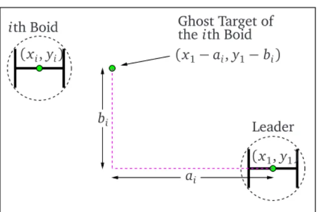
bi

a_i

(x_i,y_i)

(x1,y1) (x1−ai,y1−bi)

Leader

ith Boid

theith Boid Ghost Target of

Figure 2: Positioning of a mobile ghost target relativeto theposition oftheleader-boid.

The new leader-follower strategy

summons the boids of the flock to

follow one particular boid which is

adopted as the leader-boid. This

strategy is advocated for the very first

time via mobile ghost targets. These

ghost targets are positioned relative

to the position of the leader-boid

with a user defined Euclidean

mea-sure (Figure 2).

We note here that each follower-robot

will have a different mobile ghost

tar-get designated to it.

While the mobile ghost targets move relative to the position of the leader-boid, the

follower-boids move towards the ghost targets designated to them, at every iteration

3.1.1. Attraction to Target/Ghost Target For theith boid, we designate a target

T_i ={(x,y)∈R2_:(x−_ti1)2_{+ (y}−_ti2)2 ≤_{r t}2

i}

with center(t_i1,t_i2)and radiusr t_i. The leader-boid (i=1) will move towards its target

with center(t₁₁,t₁₂). Now, with respect to the follower-boids, the mobile ghost targets

allocated to each will be positioned relative to the position of the leader (a_i horizontal

units and b_i vertical units, see Fig. 2) and whose center is given by(t_i1,t_i2) = (x₁−

a_i,y₁−b_i), fori =2 ton.

For attraction to the target/ghost target, we shall use an attractive function of the

form

H_Ni(x) = 1

2ln(Hi+1), where

H_i(x) = (x_i−t_i1)2+ (y_i−t_i2)2+υ2

i +ω

2

i , for i=1, . . . ,n. (3.1)

While the function is the measure of the distance between the ith boid and its

target T_i, it can also be treated as a measure of its convergence. In this case, the

particular form of H_Ni(x) is sufficient to be treated as a suitable attractive potential

function required to generate attractive fields around the targets. Figure 3(a) shows

the valleys created by the attractive forces in a continuous potential field. These

mo-bile valleys, associated to the momo-bile ghost targets of the follower-boids 1 and 2, are

positioned according to user-defined measurements in the leader-follower scheme.

Similarly, there would be a valley each for the remaining flockmates and the ultimate

goal is for each follower-boid to move to its designated valley. Figure 3(b) shows the

10 20 30 40 50 60 15

20 25

30 35 0

2 4 6 8 10 12 14 16

y position

Total Potential

Target of follower−boid 2

Target of follower−boid 1

FO1 FO2

x position

(a) 3D visualization

x position

y position

10 20 30 40 50 60

15 20 25 30 35

(b) Contour Plot

Figure 3: Total potential and the ontour plot generated using the attrative potential funtion for target attration and the repulsive potential funtion for avoidane of disk-shaped obstales.

3.1.2. Auxiliary Function

To ensure that the Lyapunov function candidate vanishes when all the boids converge

to their final target configuration we design a new attractive function whose role is

purely mathematical, and hence, auxiliary. We define this auxiliary function as

G_i(x) = 1 2

”

(x_i−t_i1)2+ (y_i−t_i2)2+ (θi−ti3)2

—

≥0 , for i=1, . . . ,n, (3.2)

wheret_i3is the desired orientation of theith boid. We will multiply the function to

each of the repulsive potential field function to be designed in the following section.

3.2. Repulsive Potential Field Functions

We desire the boids to avoid all fixed and moving obstacles intersecting their paths.

Therefore, we construct obstacle avoidance functions that basically measure the

avoidance, each of these functions will appear in the denominator of the repulsive

potential field function to generate the repulsive fields around the obstacles. The

numerators will be populated by tuning parameters which may be refined for safer,

shorter and smoother trajectories. The reader is referred to [13, 14, 19] for further

explanations. Now, we describe each obstacle appearing in the constrained workspace

and design the associated avoidance function.

3.2.1. Stationary Obstacles

LetO_q,q∈ {1, . . . ,m}, represent a solid object fixed within the workspace. We provide

the following definition of the stationary obstacles

Definition 3.1. The kth stationary obstacle is a disk with center(o_k1,o_k2) and radius ro_k. Precisely, the kth stationary obstacle fixed in the workspace is the set

O_k={(z₁,z₂)∈R2_:(z₁−o_k1)2+ (z₂−o_k2)2 ≤ro_k}.

For theith boid to avoid thekth stationary obstacle, we adopt the avoidance function

W_ik(x) = 1 2

”

(x_i−o_k1)2+ (y_i−o_k2)2− ro_k+r_v2—

, fori=1, . . . ,n ; k=1, . . . ,m.

(3.3)

This positive function is the Euclidean measure of the distance between the ith boid

and thekth stationary obstacle. Now let us consider, for some constantα_ik>0

(clas-sified as a tuning parameter), fori=1 (leader-boid) andk=1 (a stationary obstacle

fixed in the workspace), the effect of the ratio α11

W11. According to the Lyapunov-based control scheme, this ratio is classified as a repulsive potential field function. If the

leader-boid approaches the stationary obstacle, then the value of the ratio will

in-crease. If it moves away from the stationary obstacle, the ratio will dein-crease.

Now, to provide the importance of the Lyapunov-based control scheme, we

artificial potential field function for system (2.1). Because, with respect to time t≥0,

one getsd L/d t ≤0 along a trajectory of (2.1), and Lis a positive definite function,L

cannot increase in t. Therefore any change in the value of the ratio could only

corre-spond to either an increase or decrease in|d L/d t|. Analogously,|d L/d t|is the rate of

dissipation of energy from the system in absolute value. If the stationary solid object

is being approached, thenW₁₁gets smaller, and the ratio gets larger. Thus, the rate of

energy dissipation, in absolute value, gets larger. This, in turn, results in an increased

activity of the system. This increased activity could only be directed towards a stable

equilibrium point, away from the stationary solid object. In other words, a situation

whereW₁₁=0 can never eventuate. Hence, if the ratio is a part of a Lyapunov

func-tion for system (2.1), then intuitively the ratio will act as a repulsive potential field

function, this is the very essence of the Lyapunov-based control scheme. An example

of the effect of the repulsive potential function designed from Equation (3.3) can be

seen in Figure 3(a). The cylindrical potential spikes are immediately evident.

Henceforth, all the obstacle avoidance functions will be appropriately coupled

with tuning parameters to design the repulsive potential field functions to generate

the collision and obstacle avoidance maneuvers.

3.2.2. Moving Obstacles

From a practical viewpoint, the control algorithms must generate feasible trajectories

based upon real-time perceptual information. In this paper, we will only consider

moving obstacles of which the system has complete and a priori knowledge. Here,

each boid itself becomes a moving obstacle for all the other boids. Therefore, for the

ith boid to avoid the jth moving boid, we consider

V_{i j}(x) = 1 2

”

(x_i−x_j)2+ (y_i− y_j)2− 2×r_v2—

This avoidance function is the measure of the Euclidean distance between theith

and the jth boid.

3.2.3. Dynamics Constraints

Again, in practice, the translational speed and the steering angle of the robots are

limited. However, in order to treat the dynamic constraints within the

Lyapunov-based control scheme we will have design anartificial obstaclecorresponding to each

dynamic constraint. Following on, we will design an appropriate obstacle avoidance

function for its avoidance.

If v_{ma x} > 0 is the maximum speed, and φ_{ma x} is the maximum steering angle

satis-fying 0< φma x < π

2 then, as shown in [14], the constraints imposed on the transla-tional and the rotatransla-tional velocities are |υ_i|< υ_{ma x} and υ2

i ≥ρ

2

minω

2

i . Whereρmin

known as theminimum turning radiusis given as ρmin =

l1

tanφma x. From above we get

|ω_i| ≤ |υi|

|ρmin| <

υma x

|ρmin| .

Based on these constraints, the following artificial obstacles can be constructed:

AO_i1={υ_i ∈R_:υi≤ −_{υmax orυi}≥_υmax}_,

AO_i2={ω_i ∈R_:ωi ≤ −_υmax/|_ρmin|_orωi ≥_υmax/|_ρmin|}_,

For avoidance, the following obstacle avoidance functions will be included:

U_i1(x) = 1

2(υma x−υi)(υma x +υi), (3.5)

U_i2(x) = 1 2

_υ ma x

|ρ_min|−ωi

υma x

|ρ_min|+ωi

, for i=1, . . . ,n. (3.6)

The repulsive potential functions generated from these obstacle avoidance functions

would guarantee the adherence to the limitations placed upon translational velocity

4. Lyapunov-based Control Scheme

Utilizing the Lyapunov-based control scheme we now design the nonlinear

con-trol laws and provide a mathematical proof that system (2.1) is indeed stable. The

control laws have been extracted from a Lyapunov function which appropriately sums

the attractive and repulsive potential field functions designed in the aforementioned

sections.

We begin with the following theorem:

Theorem 4.1. Consider a flock of nonholonomic boids, the motion of which is gov-erned by ODEs described by system (2.1). The objective is to, amongst considering other

integrated subtasks, establish and control a prescribed formation, facilitate split/rejoin

maneuvers of the boids within a constrained environment and reach the target

config-uration with the original formation. The subtasks include; restrictions placed on the

workspace, convergence to predefined targets, and consideration of kinematic and

dy-namic constraints. Utilizing the attractive and repulsive potential field functions the

following continuous time-invariant control laws can be generated for the ith boid that

per sestabilizes system (2.1) as well:

σi = −

δi1υi+ f1icosθi+ f2isinθi

/f_4i , (4.1)

ηi = −

δi2ωi+

l_l

2 −f1isinθi+f2icosθi

+ f_3i

/f5i, (4.2)

for i = 1 to n where δ_i1,δi2 > 0 are constants commonly known as convergence

parameters.

Proof:

Introducing positive constants, denoted astuning parameters,α_ik>0,β_{i j} >0 and

γis>0, fori,j,k,s∈N, we propose a Lyapunov function candidate for system (2.1):

L(x) = n X

i=1







H_N

i(x) +Gi(x)



 m X

k=1

αik

W_ik(x)

+

2

X

s=1

γis

U_is(x)

+ n X

j=1,i6=j

βi j

V_{i j}(x)

Assumption 4.1. x∗ = (t_i1,t_i2,t_i3, 0, 0, . . . ,t_n1,t_n2,t_n3, 0, 0)∈R5n ∈D(L)is an

equi-librium point of system (2.1).

Remark 4.1. This is a reasonable assumption since ˙L(x∗) = 0 making x∗ a feasible

equilibrium point, at least, in a small neighborhood of the target configuration.

Then one can easily verify the following:

1. Lis continuous and positive on the domain D_{given as}

D(L) = {x ∈R5×n: W_ik(x)>0 fori=1 ton, k=1 to m, U_is(x)>0 for

i=1 to n, s=1 to 2 and V_{i j}(x)>0 fori,j=1 to n, i6= j }.

2. L(x∗) =0, x∗∈D.

3. L(x)>0 ∀x ∈D,x 6=x∗ .

Now let us consider the time derivative of our Lyapunov function candidate L(x).

Along a particular trajectory of system (2.1), we have, upon collecting terms with v_i

andω_i separately

˙L_(2.1)(x) = n X

j=1

f_1icosθ_i+ f_2isinθ_i+ f_4iσ_i

υ_i

−

_l

1

2f1isinθi− l₁

2f2icosθi−f3i− f5iηi

ω_i

,

where functions f_1i to f_5i are defined as (on suppressingx):

f₁₁ = 1

H₁+1+

m X

k=1

α1k

W_1k + 2

X

s=1

γ1s

U_1s +

n X

j=2

β_1j V_1j

!

(x₁−t₁₁)

−

n X

i=2





1 H_i+1+

m X

k=1

αik

W_ik + 2

X

s=1

γis

U_is +

n X

j=1,i6=j

βi j

V_{i j}



(x_i−t_i1)

−G₁

n X

j=2

β_1j

V₁2_j(x1−xj) +

n X

j=2

G_jβj1

V_j2₁(xj−x1)−G1

m X

k=1

α_1k

f_1i = 



1 H_i+1+

m X

k=1

αik

W_ik + 2

X

s=1

γis

U_is +

n X

j=1,i6=j

βi j

V_{i j}



(x_i−t_i1)

−G_i

n X

j=1,i6=j

β_{i j}

V_{i j}2(xi−xj) +

n X

j=1,i6=j

G_jβji

V_ji2(xj−xi)−Gi

m X

k=1

αik

W_ik2(xi−ok1),

fori = 2 ton,

f₂₁ = 1

H₁+1+

m X

k=1

α1k

W_1k + 2

X

s=1

γ1s

U_1s +

n X

j=2

β1j

V_1j

!

(y₁−t₁₂)

−

n X

i=2





1 H_i+1+

m X

k=1

α_ik W_ik +

2

X

s=1

γ_is U_is +

n X

j=1,i6=j

βi j

V_{i j}



(y_i−t_i2)

−G₁

n X

j=2

β1j

V₁2_j(y1− yj) +

n X

j=2

G_jβj1

V_j2₁(yj− y1)−G1

m X

k=1

α1k

W₁2_k(y1−ok2),

f_2i = 



1 H_i+1+

m X

k=1

αik

W_ik + 2

X

s=1

γis

U_is +

n X

j=1,i6=j

βi j

V_{i j}



(y_i−t_i2)

−G_i

n X

j=1,i6=j

β_{i j}

V_{i j}2(yi− yj) +

n X

j=1,i6=j

G_jβji

V_ji2(yj− yi)−Gi

m X

k=1

αik

W_ik2(yi−ok2),

fori = 2 ton, and

f_3i = 

 m X

k=1

α_ik W_ik +

2

X

s=1

γ_is U_is +

n X

j=1,i6=j

β_{i j} V_{i j}



(θ_i−t_i3),

f_4i = 1

H_i+1+Gi γ_i1 U2

i1

, f_5i = 1

H_i+1+Gi γ_i2 U2

i2

,

fori = 1 ton.

Substituting the controllers given in (4.1) - (4.2) and the governing ODEs for

system (2.1) we obtain a semi-negative definite function :

˙L_(2.1)(x) =− n X

i=1

€

δ_i1υ2

i +δi2ω2i

Š

We have thus provided a working proof of the fact that _{d t}d[L(x)]≤0 ∀x ∈D.

Finally, it can easily be verified that the first partials of L(2.1)(x)isC1 which makes

up the fifth and final prerequisite of a Lyapunov function.

Once L(x)successfully meets the five prerequisites discussed above, it is declared

a feasible Lyapunov function for system (2.1) and x∗ is at least a stable equilibrium

point in the sense of Lyapunov. In our case, this practical limitation is well within the

Lyapunov framework and there is no contradiction with Brockett’s result[2] because

we have proven only stability, and not asymptotic stability. Stability means that any

solution of system (2.1) starting close to x∗ remains near it at all times.

5. Results

In this section we illustrate the effectiveness of the Lyapunov-based control scheme

and the resulting nonlinear control laws, by simulating two interesting scenarios. We

present two different split/rejoin maneuvers for a flock of ten boids clustered at the

starting line. The boids in each scenario coalesce into a distinct prescribed formation

and move in the direction of their targets. When the formation encounters fixed

ob-stacles intersecting its path, the affected boids split and move around the obob-stacles

for a collision-free avoidance. Subsequently, the boids rejoin their coherent group and

the original formation gets re-enacted before the final target position is attained.

We consider two different formations in this paper: (i) arrowhead formation, and

(ii) circular formation. In the two formations, Boid 1, situated initially at (x₁,y₁) =

(8, 24) (see Fig. 4(b)and Fig. 6(b)), acts as the leader-boid. As the leader moves

towards its target, the follower-boids will move towards the moving ghost target

des-ignated to each. These ghost targets of the follower-boids are positioned relative to

the position of the leader in a specific pattern (the scheme is illustrated in Fig.2) that

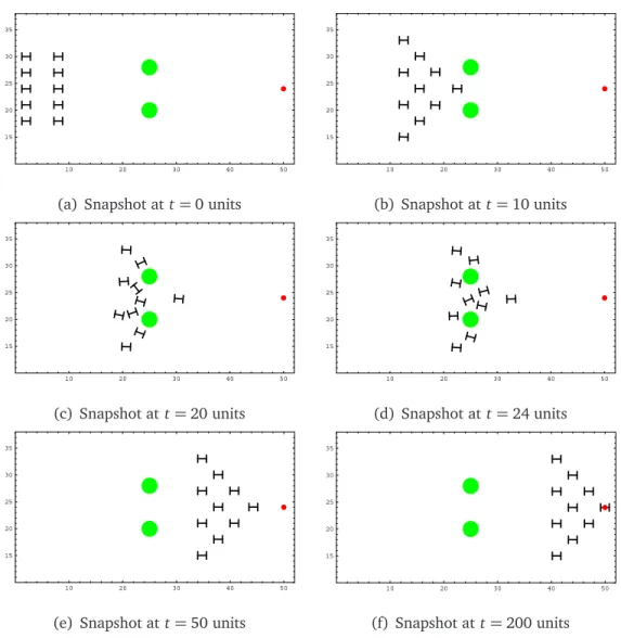
5.1. Scenario 1: Arrowhead Formation

For this scenario, the prescribed formation is an arrowhead with the leader boid

positioned at the tip of the arrowhead. Assuming the units have been appropriately

taken care of, initial conditions pertaining the kinodynamic system and other

essen-tials of the simulation are provided in Table 1.

As the leader moves towards its target, the follower-boids move towards their

ghost targets positioned relative to the leader’s position, according to the coordinates

(a_i,b_i)given in Table 1. From the initial configuration the boids quickly coalesce into

a distinct arrowhead formation (Fig. 4(b)). The boids then split from their

forma-tion to avoid two obstacles in their path (as shown in Figures 4(c) and 4(d)). After

the avoidance, the boids rejoin the flock showing the same prescribed arrowhead

for-mation (Fig. 4(e)). The reforfor-mation takes place before the flock reaches the final

configuration (Fig. 4(f))

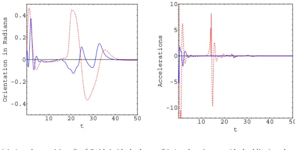
Figure 5(a) shows the evolution of the orientations of the first and the fourth

boids. The different headings can be noticed during the split of the flock,

how-ever, the pre-defined final orientations are achieved at the target configuration as

warranted in this research. Figure 5(b) shows the acceleration components for the

leader-boid. One can clearly notice the convergence of the variables at the final state

implying the effectiveness of the controllers. Similar trends were observed in the case

of the follower-boids. The profiles of the Lyapunov function along the system

trajec-tory show that the conditions of Theorem 1 have been satisfied and that the initial

Table1: Numerialvaluesof initialstates,onstraints andparametersof Senario1.

Initial Conditions

Rectangular positions (x₁,y₁) = (8, 24), (x₂,y₂) = (8, 27), (x₃,y₃) = (8, 21);

(x4,y4) = (8, 30), (x5,y5) = (2, 24), (x6,y6) = (8, 18);

(x₇,y₇) = (2, 30), (x₈,y₈) = (2, 27), (x₉,y₉) = (2, 21);

(x₁₀,y₁₀) = (2, 18)

Angular positions & velo. θ_i =0, υ_i =0.5, ω_i =0.8, fori= 1 to 10

Constraints and Parameters Dimension of Boids l₁ =1.6,l₂=1.4

Target for leader (t11,t12) = (50, 24),r t1=0.5

Final orientations t_i3=0, fori= 1 to 10

Position of ghost (a₂,b₂) = (3,−3), (a₃,b₃) = (3, 3), (a₄,b₄) = (6,−6);

targets relative to (a5,b5) = (6, 0), (a6,b6) = (6, 6), (a7,b7) = (9,−9);

leader boid (a₈,b₈) = (9,−3), (a₉,b₉) = (9, 3), (a₁₀,b₁₀) = (9, 9);

Fixed obstacles(o_k1,o_k2) (o₁₁,o₁₂) = (25, 28), (o₂₁,o₂₂) = (25, 20),ro₁ =ro₂=1.5

Max. translational speed υ_{ma x} =3

Min. turning radius ρ_min=0.14

Clearance parameter ε₁=0.1,ε₂=0.05

Control and Convergence Parameters Obstacle avoidance α_ik= 0.6, fori =1 to 10 andk =1 to 2

Boid avoidance β_{i j} = 0.01, fori =1 to 10, j =1 to 10,i6= j

Dynamics constraints γ_is =0.0001, fori =1 to 10,s =1 to 2

10 20 30 40 50 15

20 25 30 35

(a) Snapshot att=0 units

10 20 30 40 50 15

20 25 30 35

(b) Snapshot att=10 units

10 20 30 40 50 15

20 25 30 35

(c) Snapshot att=20 units

10 20 30 40 50 15

20 25 30 35

(d) Snapshot at t=24 units

10 20 30 40 50 15

20 25 30 35

(e) Snapshot att=50 units

10 20 30 40 50 15

20 25 30 35

(f) Snapshot att=200 units

10 20 30 40 50 t

-0.4 -0.2 0 0.2 0.4

Orientation

in

Radians

(a) Angular position θ of Boid 1 (dashed

line) and Boid 4.

10 20 30 40 50 t

-10 -5 0 5 10

Accelerations

(b) Accelerations:σ(dashed line) andη.

Figure 5: Evolutionof theangularpositions andaeleration omponentsfor Senario1.

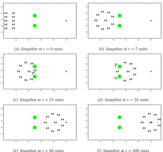
5.2. Scenario 2: Circular Formation

For this scenario, the prescribed formation is a circular arrangement with the

leader-boid positioned in the center of the formation. We retain the leader-follower

scheme although the virtual structures/centers could have been utilized for this

par-ticular formation. Table 5.2 provides the essentials for the simulation; however, only

those that are different from scenario 1.

Figure 6 illustrate a similar split/rejoin maneuver as in scenario 1; however, with

a different constellation. The flock establishes the specified formation, carries out the

split/rejoin maneuver to avoid the obstacles, re-establishes the formation and finally

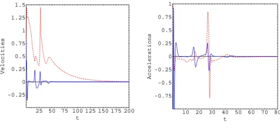
converges to the final configuration. Figure 7 shows the velocity and acceleration

components of Boid 4. Again the figures illustrate the convergent nature of the

Table2: Numerialvaluesof onstraints andparametersofSenario2.

Position of ghost (a₂,b₂) =κ(cos(π

9), sin(

π

9)),(a3,b3) =κ(cos( 17π

9 ), sin( 17π

9 ))

targets relative to (a₄,b₄) =κ(cos(π

3), sin(

π

3)),(a5,b5) =κ(cos(π), sin(π)) leader boid (a₆,b₆) =κ(cos(5π

3 ), sin( 5π

3 )),(a7,b7) =κ(cos( 5π

9 ), sin( 5π

9 ))

(a₈,b₈) =κ(cos(7π

9 ), sin( 7π

9 )),(a9,b9) =κ(cos( 11π

9 ), sin( 11π

9 ))

(a₁₀,b₁₀) =κ(cos(13π

9 ), sin( 13π

9 ))whereκ=7 Control and Convergence Parameters Obstacle avoidance αik =0.6, fori =1 to 10 and k=1 to 2

Boid avoidance β_{i j} =0.01, fori =1 to 10, j= 1 to 10,i6= j

Dynamics constraints γis= 0.001, fori =1 to 10 ands =1 to 2

10 20 30 40 50 15

20 25 30 35

(a) Snapshot att=0 units

10 20 30 40 50 15

20 25 30 35

(b) Snapshot att=7 units

10 20 30 40 50 15

20 25 30 35

(c) Snapshot att=15 units

10 20 30 40 50 15

20 25 30 35

(d) Snapshot at t=35 units

10 20 30 40 50 15

20 25 30 35

(e) Snapshot att=60 units

10 20 30 40 50 15

20 25 30 35

(f) Snapshot att=200 units

25 50 75 100 125 150 175 200 t

-0.25 0 0.25 0.5 0.75 1 1.25 1.5

Velocities

(a) Velocities:υ(dashed line) andω.

10 20 30 40 50 60 70 80

t -0.75

-0.5 -0.25 0 0.25 0.5 0.75 1

Accelerations

(b) Accelerations:σ(dashed line) andη.

Figure7: Evolutionof theveloityandaeleration omponentsof Boid4for Senario2.

6. Conclusion

The Lyapunov-based control scheme was successfully utilized to create a new set

of continuous time-invariant control laws. We were able to generate a prescribed

for-mation, accomplish the required split/rejoin maneuvers and re-establish the original

formation of a flock of nonholonomic robots. By and large, the control scheme has

presented an excellent platform to yield split/rejoin maneuvers of a flock fixed in a

ar-bitrary formation. The new controllers (4.1) and (4.2) produced feasible trajectories

and ensured a nice convergence of the system to the equilibrium state, whilst

satis-fying all the constraints tagged on the system. Moreover, although computationally

intensive the control scheme will sufficiently encompass expansions to and scalability

of flocks.

The unique pattern of boids’ movement as a flock was possible by inclusion of

posi-tioned relative to the leader-boid. This specific positioning, however, restricted the

formation to a horizontal wayward motion only. Future research will address rotation

of formations and changing the leadership roles of the flockmates. The authors will

also utilize the concept of flocking via the Lyapunov-based control scheme on tunnel

passing and lane merging problems of intelligent vehicle systems.

References

[1] C. Belta and V. Kumar. Abstraction and control for groups of robots. InReprinted from

IEEE Transactions on Robotics and Automation, volume 4, pages 865–875, October 2004.

[2] R.W. Brockett. Differential Geometry Control Theory, chapter Asymptotic Stability and

Feedback Stabilisation, pages 181–191. Springer-Verlag, 1983.

[3] D. E. Chang, S. C. Shadden, J. E. Marsden, and R. Olfati-Saber. Collision avoidance for

multiple agent systems. In Procs. of the 42nd IEEE Conference on Decision and Control,

Maui, Hawaii USA, December 2003.

[4] D. Crombie. The examination and exploration of algorithms and complex behavior to

realistically control multiple mobile robots. Master’s thesis, Australian National

Univer-sity, 1997.

[5] P. ¨Ogren. Formations and obstacle avoidance in mobile robot control. Master’s thesis,

Royal Institute of Technology, Stockholm, Sweden, June 2003.

[6] L. Edelstein-Keshet. Mathematical models of swarming and social aggregation. In

Procs. 2001 International Symposium on Nonlinear Theory and Its Applications, pages

1–7, Miyagi, Japan, October-November 2001.

[7] G. H. Elkaim and R. J. Kelbley. A lightweight formation control methodology for a

swarm of non-holonomic vehicles. InIEEE Aerospace Conference, 2006.

[8] V. Gazi. Swarm aggregations using artificial potentials and sliding mode control. In

Procs. IEEE Conference on Decision and Control, pages 2041–2046, Maui, Hawaii,

[9] W. Kang, N. Xi, J. Tan, and Y. Wang. Formation control of multiple autonomous robots:

Theory and experimentation. Intelligent Automation and Soft Computing, 10(2):1–17,

2004.

[10] J-C. Latombe. Robot Motion Planning. Kluwer Academic Publishers, USA, 1991.

[11] M. Lindh´e. A flocking and obstacle avoidance algorithm for mobile robots. Master’s

thesis, KTH School of Electrical Engineering, Stockholm, Sweden, June 2004.

[12] C. W. Reynolds. Flocks, herds, and schools: A distributed behavioral model, in computer

graphics. InProcs. of the 14th annual conference on Computer graphics and interactive

techniques, pages 25–34, New York, USA, 1987.

[13] B. Sharma. New directions in the applications of the lyapunov-based control scheme to

the findpath problem. PhD Dissertation, July 2008.

[14] B. Sharma and J. Vanualailai. Lyapunov stability of a nonholonomic car-like robotic

system. Nonlinear Studies, 14(2):143–160, 2007.

[15] B. Sharma, J. Vanualailai, and A. Prasad. Formation control of a swarm of mobile

manipulators. Rocky Mountain Journal of Mathematics, To Appear.

[16] H. Tanner, A. Jadbabaie, and G. J. Pappas. Stable flocking of mobile agents, part i:

Fixed topology. In Procs. of the 42nd IEEE Conference on Decision and Control, pages

2010–2015, 2003.

[17] R. Olfati-Saber. Flocking for multi-agent dynamic systems: Algorithms and theory.IEEE

Transactions on Automatic Control, 51(3):401–420, 2006.

[18] R. Olfati-Saber and R. M. Murray. Flocking with obstacle avoidance: Cooperation with

limited information in mobile networks. InProcs. of the 42nd IEEE Conference on

Deci-sion and Control, volume 2, pages 2022–2028, Maui, Hawaii, December 2003.

[19] J. Vanualailai, B. Sharma, and A. Ali. Lyapunov-based kinematic path planning for a

3-link planar robot arm in a structured environment. Global Journal of Pure and Applied