The Numerical Solution of Partial Differential-Algebraic Equations (PDAEs) By Multivariate Pade Approximation

Vol. 4, No. 1, 2011, 67-75

ISSN 1307-5543 – www.ejpam.com

The Numerical Solution Of Partial Differential-Algebraic

Equa-tions (PDAEs) By Multivariate Pade Approximation

Muhammed Yi˘

gider

_{, Ercan Celik}

1_{Department of Mathematics, Faculty of Science, Ataturk University, Erzurum, Turkey}

2_{Department of Mathematics, Faculty of Art and Science, Erzincan University, Erzincan, Turkey}

Abstract. In this paper, Numerical solution of Partial Diferential-Algebraic Equa- tions(PDAEs) is con-sidered by Multivariate Padè Approximations. We applied these method to one example. First Partial Diferential-Algebraic Equation(PDAE) has been converted to power series by two-dimensional difer-ential transformation,Then the numerical solution of equation was put into Multivariate Padè series form. Thus we obtained numerical solution of Partial Diferential-Algebraic Equa- tion(PDAE).

2000 Mathematics Subject Classifications: 35

Key Words and Phrases: Partial Differential-Algebraic Equation (PDAs), two-dimensional differential transformation, Multivariate Padè Approximation

1. Introduction

In this study, we consider Linear Partial Differential-Algebraic Equations(PDAEs) of the form

Au_t(t,x) +Bu_{x x}(t,x) +Cu(t,x) = f(t,x) (1) Wheret∈(0,t_e)andx ∈(−l,l)⊂R,A,B,C ∈Rnxnare constant matrices,

u,f : 0,t_e

x[−l,l]→Rn. We are interested in cases where at least one of the matrices A andBis singular. The two special casesA=0 orB=0 lead to ordinary differential equations or DAEs which are not considered here. Therefore in this paper we assume that none of the matricesAorB is the zero matrix[6, 7].

Many important mathematical models can be expressed in terms of Partial Differential Alge-braic Equations(PDAEs). Such models arise in many areas of mathematics, engineering, the physical sciences and population growth. In resent years, much research has been focused on the numerical solution of Partial Differential-Algebraic Equations(PDAEs). Some numerical methods have been developed, using Runge-Kutta methods[8].

∗_{Corresponding author.}

Email addresses:erelikatauni.edu.tr(E. Celik),myigidererzinan.edu.tr(M. Yigider)

M. Yi˘gider, E. Çelik Eur. J. Pure Appl. Math,4(2011), 67-75 68

The purpose of this paper is to consider the numerical solution of Partial Differential-Algebraic Equations(PDAEs) by using Multivariate Padé Approximations.

2. Two-Dimensional Differential Transformation

The basic definition of the two-dimensional differential transform is defined as follows

[9, 2, 3, 4, 1]:

W(k,h) = 1

k!h! –

∂k+h_w(x,y) ∂_xk_∂yh

™

0,0

(2)

wherew(x,y)is the original function andW(k,h)is the transformed function. The transfor-mation is calledT- function and lower case and upper case letters represent the original and transformed functions respectively. The differential inverse transform ofW(k,h)is defined as

w(x,y) =

∞ X

k=0

∞ X

h=0

W(k,h)xkyh (3)

and from Eqs.(2) and (3) can be concluded

w(x,y) =

∞ X

k=0

∞ X

h=0

1 k!h!

–

∂k+h_w(x,y) ∂_xk_∂yh

™

0,0

xkyh. (4)

3. Multivariate Padé Approximations

Consider the bivariate function f(x,y)with Taylor series development

f(x,y) =

∞ X

i,j=0

ci jxiyj (5)

around the origin. We know that a solution of univariate Padé approximation problem for

f(x) =

∞ X

i=0

cixi (6)

is given by

p(x) =

Pm

i=0cixi x

Pm−1

i=0 cixi · · · xn

Pm−n i=0 cixi

c_m+1 cm · · · cm+1−n

..

. ... ... ...

c_m+n c_m+n−1 · · · c_m

(7)

and

q(x) =

1 x · · · xn

c_m+1 c_m · · · c_m+1−n ..

. ... . .. ... c_m+n c_m+n−1 · · · c_m

Let us now multiply jth row in p(x) andq(x) by xj+m−1 (j =2, . . . ,n+1) and afterwards divide jth column inp(x)andq(x)by xj−1(j=2, . . . ,n+1). This results in a multiplication of numerator and denominator byxmn. Having done so, we get

p(x)

q(x)=

Pm

i=0cixi

Pm−1

i=0 cixi · · ·

Pm−n

i=0 cixi

c_m+1xm+1 c_mxm · · · c_m+1−nxm+1−n ..

. ... . .. ...

c_m+nxm+n c_m+n−1xm+n−1 · · · c_mxm

1 1 · · · 1

cm+1xm+1 cmxm · · · cm+1−nxm+1−n

..

. ... . .. ...

cm+nxm+n cm+n−1xm+n−1 · · · cmxm

(9)

(D=detD_m,n6=0).

This quotient of determinants can also immediately be written down for a bivariate function f(x,y). The sumP_ik₌₀cixishall be replacedkth partial sum of the Taylor series development

of f(x,y)and the expressionc_kxkby an expression that contains all the terms of degreekin f(x,y). Here a bivariate termc_{i j}xiyjis said to be of degreei+j.

If we define

p(x,y) =

Pm

i+j=0ci jxiyj

Pm−1

i+j=0ci jxiyj · · ·

Pm−n

i+j=0ci jxiyj

P

i+j=m+1ci jxiyj

P

i+j=mci jxiyj · · ·

P

i+j=m+1−nci jxiyj

..

. ... . .. ...

P

i+j=m+nci jxiyj

Pm

i+j=m+n−1ci jxiyj · · ·

Pm

i+j=mci jxiyj

(10) and

q(x,y) =

1 1 · · · 1

P

i+j=m+1ci jxiyj

P

i+j=mci jxiyj · · ·

P

i+j=m+1−nci jxiyj

..

. ... ... ...

P

i+j=m+nci jxiyj

Pm

i+j=m+n−1ci jxiyj · · ·

Pm

i+j=mci jxiyj

(11)

Then it is easy to see thatp(x,y)andq(x,y)are of the form

p(x,y) =P_imn_+j+₌m_mnai jxiyj

q(x,y) =P_imn_+j+₌n_mnbi jxiyj

(12)

We know that p(x,y) andq(x,y) are called Padé equations [5]. So the multivariate Padé approximant of order(m,n)for f(x,y)is defined as,

rm,n(x,y) =

p(x,y)

M. Yi˘gider, E. Çelik Eur. J. Pure Appl. Math,4(2011), 67-75 70

4. Numerical Example:

The test problem considers the following Partial Differential-Algebraic Equation(PDAE)

[8]:



 

0 1 0 0 0 1 0 0 0



 ut+



 

0 0 −1

0 −1 −1

0 0 0



 ux x+



 

−1 −1 −1

0 −1 0

0 0 1





u= f (14)

x ∈[−0.5, 0.5],t∈[0, 1]. Where

f₁ = −x(x−1)(2 sint+cost)−(et+t5)(x2−x+2)

f2 = x(x−1)(et+5t4−cost)−2(et+t5+cost)

f₃ = −x(x−1)(et+t5).

The exact solution is

u(x,t) =



 

x(x−1)sin(t)

x(x−1)cos(t)

x(x−1)(et+t5)





 (15)

Equivalently, Equation (14) can be written as



 

0 1 0 0 0 1 0 0 0

     

u_1t u_2t u3t

  +   

0 0 −1

0 −1 −1

0 0 0

     

u_{1x x} u_{2x x} u3x x

  +   

−1 −1 −1

0 −1 0

0 0 1

      u₁ u₂ u3   =    f₁ f₂ f3    (16) u_2t−u_{3x x}−u₁−u₂−u₃= f₁

u_3t−u_{2x x}−u_{3x x}−u₂= f₂ (17) −u₃= f₃

By using the basic definition of the two-dimensional differential transform and taking the transform of Equation (17) can obtain that

(k+1)U2(k+1,h)−(h+1)(h+2)U3(k,h+2)−U1(k,h)−U2(k,h)−U3(k,h) =F1(k,h) (k+1)U3(k+1,h)−(h+1)(h+2)U2(k,h+2)−(h+1)(h+2)U3(k,h+2)−U2(k,h) =F2(k,h)

−U₃(k,h) =F₃(k,h)

Consequently, by substituting the values ofU_i. We have obtained

u₁(x,t) =−x t+x2t+1

6x t

3₋1

6x

2_t3₋ 1

120x t

5₊ 1

120x

2_t5₊ 1

5040x t

7

u₂(x,t) =−x+x2+1

2x t

2₋1

2x

2_t2₋ 1

24x t

4₊ 1

24x

2_t4₊ 1

720x t

6₋ 1

720x

2_t6

u₃(x,t) = −x−x t+x2−1 2x t

2_+x2_t−1

6x t

3₊1

2x

2_t2₋ 1

24x t

4₊1

6x

2_t3₋ 121

120x t

+ 1

24x

2_t4₋ 1

720x t

6₊121

120x

2_t5₋ 1

5040x t

7₊ 1

720x

2_t6

The Power seriesu₁(x,t),u₂(x,t)andu₃(x,t)can be transformed into multivariate Padé ap-proximation

m=3,n=2

p1(x,t) =

−x t+x2t −x t 0

1 6x t

3 _x2_{t −x t} 1

6x

2_t3 1 6x t

3 _x2_t

= −0.1666666667x3t5+0.1666666667x4t5−x5t7+x6t7

q₁(x,t) =

1 1 1

1 6x t

3 _x2_{t −x t} 1

6x 2_t3 1

6x t 3 _x2_t

= x4t2+0.1666666667x2t4+0.02777777778x2t6+0.1666666667x4t4

r₁(x,t) = p1(x,t)

q₁(x,t)

= −0.1666666667x

3_t5_{+0.1666666667x}4_t5_−x5_t7_+x6_t7

x4t2+0.1666666667x2t4+0.02777777778x2t6+0.1666666667x4t4

p2(x,t) =

−x+x2+1 2x t

2 _−x+x2 _−x

−1 2x

2_t2 1

2x t

2 _x2

−1 24x t

4 ₋1

2x 2_t2 1

2x t 2

= −0.2500000000x3t4−0.5000000000x5t2+0.04166666667x4t4

+0.5000000000x6t2+0.1041666667x3t6+0.2083333333x5t4

q2(x,t) =

1 1 1

−1 2x

2_t2 1 2x t

2 _x2

−1 24x t

4 ₋1 2x

2_t2 1 2x t

2

= 0.2500000000x4t4+0.5000000000x4t2+0.2500000000x4t4

+0.20833333333x3t4+0.0208333333x2t6

r2(x,t) =

p₂(x,t)

M. Yi˘gider, E. Çelik Eur. J. Pure Appl. Math,4(2011), 67-75 72

=

‚

−0.2500000000x3t4−0.5000000000x5t2+0.04166666667x4t4

+0.5000000000x6t2+0.1041666667x3t6+0.2083333333x5t4 Œ

‚

−0.2500000000x3t4−0.5000000000x5t2+0.04166666667x4t4

+0.5000000000x6t2+0.1041666667x3t6+0.2083333333x5t4 Œ

p3(x,t) =

−x−x t+x2−1₂x t2+x2t −x−x t+x2 −x −1

6x t 3₊1

2x

2_t2 ₋1

2x t

2_+x2_{t −x t+x}2

−1 24x t

4₊1 6x

2_t3 ₋1

6x t 3₊1

2x

2_t2 ₋1 2x t

2_+x2_t

=0.0833333333x2t4−0.3333333333x3t3+0.50000000000x4t2+0.0694444444x2t6 −0.0416666667x3t5−0.0416666667x2t5+0.2083333333x3t4+0.083333333x4t4

−0.3333333333x4t3

r₃(x,t) = p3(x,t)

q3(x,t)

=



 

0.2083333333x4t4−0.0833333333x3t4−0.5000000000x5t2+0.5000000000x6t2 −0.0694444444x3t6−0.1250000000x5t4+0.3333333333x4t3−0.0416666667x3t5

−0.5000000000x5t3+0.0416666667x4t5+0.1666666667x6t3



 



 

0.0833333333x2t4−0.3333333333x3t3+0.50000000000x4t2+0.0694444444x2t6 −0.0416666667x3t5−0.0416666667x2t5+0.2083333333x3t4+0.083333333x4t4

−0.3333333333x4t3



 

Table1: ComparisonoftheNumerialSolutionofu1(x,t)withExatSolutions(t=0.01)

x u1(x,t) r1(x,t)

u₁(x,t)−r₁(x,t) -0.5 0.007499875000 0.007499874999 1.10-12

-0.4 0.005599906667 0.005599006668 1.10-12 -0.3 0.003899935000 0.003899935000 0 -0.2 0.002399960000 0.002399960000 0 -0.1 0.001099981667 0.001099981668 1.10-12

Table2: Comparisonofthenumerialsolutionofu

2(x,t)withexatsolutions(t=0.01)

x u2(x,t) r2(x,t)

u₂(x,t)−r₂(x,t) -0.5 0.07499625003 0.07499625011 8.10-10

-0.4 0.5599720002 0.5599720006 4.10-10 -0.3 0. 3899805002 0. 3899805002 2.10-10 -0.2 0.2399880001 0.2399880002 1.10-10 -0.1 0.1099945000 0.1099945001 1.10-10 0.1 -0.08999550004 -0.08999550002 2.10-11 0.2 -0. 1599920001 -0. 1599929999 2.10-10 0.3 -0.2099895001 -0.2099895999 2.10-10 0.4 -0.2399880001 -0.2399889999 2.10-10 0.5 -0.2499875001 -0.2499874995 6.10-10

Table3: Comparisonofthenumerialsolutionofu

3(x,t)withexatsolutions(t=0.01)

x u₃(x,t) r₃(x,t) u ₃(x,t)−r₃(x,t) -0.5 0.7575376252 0.7575376251 1.10-10

-0.4 0.5656280935 0.5656280938 3.10-10 -0.3 0. 3939195651 0. 3939195651 0 -0.2 0.2424120401 0.2424120401 0 -0.1 0.1111055184 0.1111055184 0

0.1 -0.09090451503 -0.09090451504 1.10-11 0.2 -0. 1616080267 -0. 1616080267 0 0.3 -0.2121105351 -0.2121105350 1.10-10 0.4 -0.2424120401 -0.2424120401 0 0.5 -0.2525125418 -0.2525125415 3.10-10

Figure1: Valuesofu

1(x,t)andits r

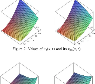
Figure2: Valuesofu

2(x,t)andits r

3,2(x,t)

Figure3: Valuesofu3(x,t)andits r3,2(x,t)

5. Conclusions

The method has proposed for solving partial differential-algebraic equations(PDAEs). The results of example showed that exactly the same solutions have been obtained with Multivarite Padé approximation. On the other hand the results are quite reliable. Therefore, this method can be applied to many complicated Partial Differential-Algebraic Equations(PDAEs).

References

[1] G Adomian. Convergent series solution of nonlinear equations, Journal of Computational and applied Mathematits, 11, 225-230,1984.

[2] F Ayaz. On the Two-Dimensional Differential Transform Method, Applied Mathematics and Computation, 143:361-374,2003.

[4] N Bildik, A Konuralp. Two-Dimensional Differential Transform Method,Adomian’s De-compostion Method and Variational Iteration Method for Partial Differential Equations, International Journal of Computer Mathematics ,Vol.83, 12:973-987,2006.

[5] A Cuyt, L Wuytack. Nonlinear Methods in Numerical Analysis, Amsterdam,1987.

[6] W Lucht, K Strehmel, C E Liebenow. Linear Partial Differential-Algebraic Equations, Part I, Reports of the Institute of Numerical Mathematics, Report No. 17,1997.

[7] W Lucht, K Strehmel, C E Liebenow. Linear Partial Differential-Algebraic Equations, Part II, Reports of the Institute of Numerical Mathematics, Report No. 18, 1997,

[8] K Strehmel, K Debrabant. Convergence of Runge-Kutta Methods Applied to Linear Partial Differential-Algebraic Equations, Applied Numerical Mathematics, 53:213-229, 2005,