A Patient-speci
fi
c Knee Joint Computer
Model Using MRI Data and ‘in vivo’
Compressive Load from the Optical Force
Measuring System
Bo
zidar Poto
ˇ
cnik
ˇ
1, Damjan Zazula
1, Boris Cigale
1, Du
ˇ
san Heric
1, Edvard
Cibula
1and Toma
z Toma
ˇ
zi
ˇ
c
ˇ
21Faculty of Electrical Engineering and Computer Science, University of Maribor, Slovenia
2University Clinical Centre of Maribor, University of Maribor, Slovenia
Modelling of patient knee joint from the MRI data and simulating its kinematics is presented. A flexion of the femur with respect to the tibia from 0◦ to around
40◦ is simulated. The finite element knee model is
driven by compressive load measured ‘in vivo’ during MRI process by using specially developed optical force measurement system. Predicted kinematics is evaluated against the high-quality model obtained by registration from experimentally gathered low-quality MRI at fixed flexions. Validation pointed out that the mean square error (MSE) for the Euler rotation angles are bellow 1.73◦, while the MSE for Euler translation is smaller
than 5.93 mm.
Keywords: compressive load, computer model, finite elements, knee joint, optical force sensor
1. Introduction
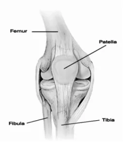
The knee joint is the largest and heavily loaded joint in the human body. Figure 1 depicts the knee joint with three main bones: bone femur, bone tibia, and bone patella. Consequently, the knee joint is highly susceptible to incidences of injuries and osteoarthrosis. Knowledge of ‘in vivo’ joint motion and loading during func-tional activities is, therefore needed to improve our understanding of knee joint degeneration and restoration. Such system for knee joint kinematics analysis and/or simulation should be able to deal with specificity of particular in-dividuals. One possibility is motion analysis systems which expand our understanding of the
mechanics of normal and pathological human movement(Rowe et al., 2000). Another pos-sibility is human knee computer models, which also present an effective way of evaluating these characteristics during the design phase, and pro-vide an indication of expected clinical perfor-mance (Bei and Fregly, 2004; Halloran et al., 2005).
Figure 1.Human knee joint with main bones.
3)evaluating the movement of markers attached to the skin, 4) evaluation of external markers invasively attached to the bone, 5) cadaveric dissection studies, 6) 2D fluoroscopic motion measurement using bone models, and 7) eval-uation of 2D images from computed tomog-raphy (CT) and magnetic resonance imaging (MRI) (Patel et al., 2004; Piazza and Cavanagh, 2000; Freeman and Piskernikova, 2005). Mea-surement methods using markers attached to the skin or bone-implanted markers have been proven to be accurate enough to collect slow ‘in vivo’ knee joint dynamics(Beillas et al., 2004; Rowe et al. 2000; Jan et al., 2002; Schuler et al., 2005; Zhou et al., 2002). However, de-vices attached directly to the skin(e.g. optical skin markers) can incur errors due to relative motion between the skin and the bone. Tran-scutaneous bone pins can loosen, bend and/or interfere with normal muscle action (Schuler et al., 2005). Roentgen stereophotogrammet-ric analysis, and MR/CT imaging are normally gathered quasi-statically due to equipment lim-itations, and, thus, do not permit dynamic ana-lysis. This can partially be overcome by using an open MR scanner. Several studies measur-ing kinematics indirectly from MRI data while a knee was loaded with constant weight have been recently reported(Patel et al., 2004; Rothe et al., 2004). The 2D fluoroscopic motion mea-surement methods have clear advantages as they do not need markers and enable a direct mea-surement of bone motion, however, the main drawback is the need for radiation.
A number of computer models, recently finite element (FE) models, have been developed to study knee joint mechanics (Halloran et al., 2005). These models are usually based on a 3D reconstruction of the knee joint from some modality imaging data(e.g. MRI or CT)or spe-cial 3D laser coordinate digitizing system(e.g. in Donahue et al., 2003). Additional data, such as material properties are then used to supple-ment these models. Some functional activities, e.g. full gait cycle in (Godest et al., 2002) or one-legged forward hopping in (Beillas et al., 2004), are then simulated, and the knee joint responses in terms of kinematics and pressure data are obtained. The simulation tools used are either commercial such as PAM-SAFE(ESI Group, Paris, France)or ABAQUS (ABAQUS Inc.,USA) (Bei and Fregly, 2004; Halloran et al., 2005; Godest et al., 2002) or specially
designed numerical problem solvers ( Abdel-Rahman and Hefzy, 1998). The quality of the predictions made by these models is largely dependent on the quality of the experimental data (e.g. loads) used to drive them (Beillas et al., 2004). FE models are usually evaluated against some ‘in vitro’ data from other studies, experimental data from kinematics measuring systems or, recently, ‘in vivo’ kinematics data (e.g. Beillas et al., 2004). A recent attempt at real-time model simulation is reported in (Jan et al., 2002), where this method actually visual-izes, rather than just simulates, a 3D joint model driven by experimental kinematics data.
To the best of our knowledge, only a few com-puter models exist, based on actual ‘in vivo’ pa-tient’s data, i.e. anatomy and specific ‘in vivo’ kinematics. The first such approach is revealed in (Beillas et al., 2004), where a quality FE knee model of a male patient performing a one-legged forward hopping trail was constructed. The kinematics data driving this model was ob-tained during hopping by an ‘in vivo’ motion measuring system.
field was refined and accurately validated. Mi-nor modifications were also done in template knee-joint FE model, especially by model of MR exercise rig. The material and structural properties of knee joint structures were stud-ied in greater detail once again. Some param-eters were, consequently, fine tuned. Proposed modelling approach was thoroughly assessed on knee-joints of two patients. Both knee-joints were fully modelled and simulated by using patient-specific MRI data. Quantitative mea-sures were introduced to assess this computer model quality. A special procedure for deter-mining the Euler translation error was devel-oped as well.
2. Experimental Methods
2.1. Patient Imaging Data Acquisition
Two male volunteers were examined (aged 22 and 52 years), having signs on meniscus or ligament tear. Imaging material was acquired using a traditional 1.5 T MR scanner (Visart, Toshiba, Tokyo, Japan). A knee joint of each patient was scanned twice, namely: 1) with high-quality static MR protocol and 2) with low-quality static MR protocol repeated at a few different fixed knee flexions.
High-quality static MR protocol was established to ease the 3D reconstruction of the patient’s knee joint. This protocol uses a FE3D image technique with the quadrature (QD) knee coil
of an MR scanner(TR 41 ms, TE 9 ms, flip an-gle 18/73, NAQ 1). Image acquisition was per-formed in sagittal orientation with 2 mm slice thickness. The field of view(FOV)was 22 x 22 cm with in-plane resolution of 0.43 mm(output image matrix was 512 x 512 pixels). Acqui-sition time was around 22 minutes for a se-quence consisting of 60 slices(cross-sections). The patient’s knee was slightly supported dur-ing static MR protocol, thus provokdur-ing approx-imately 10◦knee flexion.
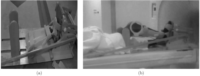
The purpose of acquiring a sparse sequence of MR images at a few fixed flexions was to per-mit the evaluation of the kinematic behaviour of the FE knee joint model. A patient with a flexed knee exerts a light force by pushing on a foot pedal during this imaging protocol (see Figure 2b). The MR data and ‘in vivo’ com-pressive load data are acquired simultaneously. The patient is scanned for up to 6 different knee flexion positions. This protocol uses a FE2D image technique with the joint pair knee coil of an MR scanner(TR 245 ms, TE 15 ms, flip angle 90, NAQ 1, gap 0.8). Only 9 slices of 4.3 mm thicknesses were acquired in sagittal orientation at each knee flexion position. The FOV was 17 x 17 cm with an in-plane resolu-tion of 0.66 mm(the output image matrix was 256 x 256 pixels). The acquisition time with this fast protocol was less than 2 minutes per flexion position.
A special MR compliant exercise rig was de-signed for this protocol (see Figure 2a, con-struction details are in(Simbio project, 2003)).
(a) (b)
Figure 2.MR compliant exercise rig: a)basic components: wooden base and flexible ankle-foot orthosis integrated within the pedal, b)patient during scanning exerts light force to the pedal comprising the integrated force measuring
The rig’s basis is an adjustable, with respect to the patient’s height, wooden board with a shoul-der support (support is not shown). The two main parts are attached to the board: 1)a flex-ible ankle-foot orthosis for fastening shank and ankle, and 2) a wooden pedal. The pedal, on the one hand, enables the setting of 6 different knee flexion angles; on the other hand, it also measures the force (compressive load) the pa-tient is exerting during imaging. Measurements are carried out by an integrated optical sensor. A flexion position can be selected manually by a small handle mounted on the pedal. Angles vary with respect to the patient’s leg length but, generally, are in the range from 0◦to 60◦flexion
with 8◦to 10◦increments.
2.2. System for Force Measurement in a Magnetic Field
When being scanned at predefined fixed knee flexions, the patient pushes his foot slightly against the pedal of the exercise rig. This com-pressive load on the foot is measured and, sub-sequently, used in the modelling phase. There-fore, a simple and fully electrical passive force measurement system was developed that can operate in those environments where magnetic fields exceed 1T. Special attention was devoted to the exclusive use of dielectric materials and, thus, the designed system does not induce any magnetic field distortions.
The presented force sensor design is based on displacement measurement by macrobend loss effect in single mode fibres(Gauthier and Ross, 1997; Donlagic and Culshaw, 2000; Gambling et al., 1978; Sharma et al., 1984). The main sensing element is a small fibre optic coil that is perturbed(squeezed)under applied force.
rubber block
single-mode fibre sensing coil initial coil bend
adjustment
pedal force
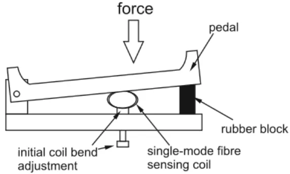
Figure 3.Mechanical configuration of the force sensor.
The practical mechanical design of the sensor is shown in Figure 3. The patient depresses the specially designed wooden pedal containing the sensing fiber coil. The elastic element(rubber block)was used between the pedal and the rest of the support structure, to convert the force asserted by the patient’s foot to the pedal dis-placement. This displacement decreases a local bend radius of the fiber at horizontal edges of the sensing coil and thus increases the optical loss within the sensing coil(thereby it decreases intensity ratio of the light at the outputs of the sensing and reference fiber branches).
This system was calibrated to measure the nor-mal component of the force asserted to the cen-ter of the pedal. The total range of the system was 0–240 N, but other force ranges could be also covered by adjustment of the properties of the elastic element that converts force to dis-placement. The resolution was better than 0.5 N. After the calibration, the absolute accuracy of the sensor proved to be better than ± 7 N. Measurements and calibration were performed at room temperature(25±5C)and relative hu-midity in the range from 40-60 %.
3. Computational Methods
3.1. Image Processing and 3D Reconstruction
A 3D knee joint is reconstructed from high-quality static 2D patient MR imaging data by using non-linear registration, developed at the University of Sheffield during the SimBio pro-ject(Simbio project, 2003; Wood et al., 2002). Image registration was applied for two reasons: 1) the edges of the knee structures are weak, and 2)integration of prior knowledge is simple and efficient.
(a) (b) (c)
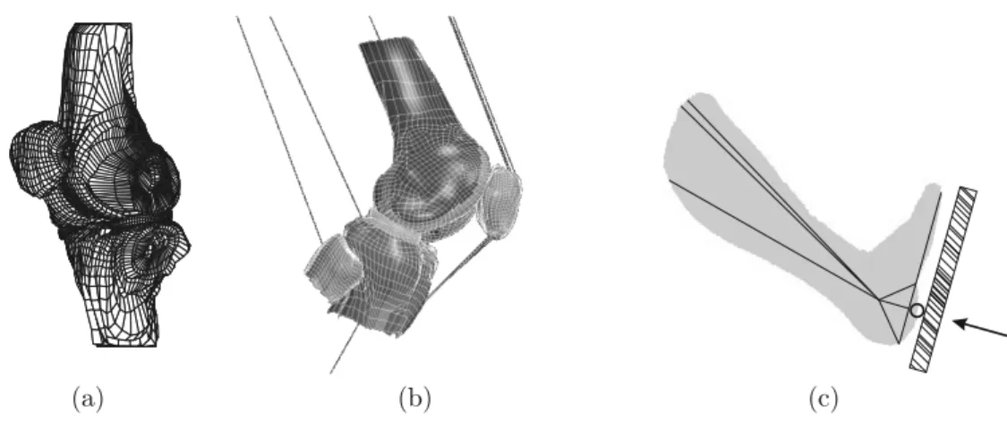
Figure 4. Knee joint model: a)template knee mesh consisting of eight structures: bones tibia, femur, patella and their corresponding cartilages, medial and lateral meniscus; b)patient-specific FE model; and c)lower leg and MR
exercise rig model.
for the template knee mesh is denoted as tem-plate image. It was built from healthy male-volunteer knee data. The template knee mesh could generally be treated as the mesh of an ave-rage human knee (e.g. an averaged European knee).
Subsequently, the constructed template knee mesh is transformed/mapped into a patient 3D knee joint mesh based on the high-quality 2D patient MR data (patient image). The map-ping function, having both a global and a local part, is determined by registration of the tem-plate image to patient image. A quality mea-sure for goodness-of-fit between both images is based on the sum-of-squares of the differ-ences in voxel grey-level intensities. The de-scribed registration and mapping of a template knee produce high-quality patient-specific 3D knee meshes. This reconstruction is completely automated.
3.2. Template 3D Knee Joint FE Model
The template 3D knee joint mesh beside bones, their cartilages and menisci comprises also other knee structures like e.g. ligaments and tendons. This template is actually the mesh from finite elements. The explicit FE code, PAM-SAFETM, is used in the modelling process. The final tem-plate mesh consisted of 3464 8-node hexahedral solid elements, 13120 shell elements, the ma-jority of which were included as part of a rigid body and the remainder used in the contact in-terface definition, and 232 bar/beam elements.
This template model was developed at the Uni-versity of Sheffield during the SimBio project (Simbio project, 2003)based on their previous knee model(Penrose et al., 2002). Brief sum-mary of this model will be given later in the text, including all minor model modifications carried out in this work.
Let us recapitulate the template properties. Three main knee bones, i.e. femur, tibia and patella, and part of the fibula are defined as rigid bodies to avoid deformations. For the same rea-son, the lateral and medial menisci are rigid bodies, as well. These bodies are in contact, thus defining contact surfaces. Seven such con-tacts are in our model: patella, femur-meniscus, tibia-femur-meniscus, and femur-tibia(two anterior and two posterior contacts). For each contact ‘master’ and ‘slave’ surfaces were fined. The articular cartilages of bones are de-fined as elastic plastic solids. Bars are used to link the anterior and posterior horns of the menisci to the tibia–104 bars for the lateral meniscus and 90 for the medial meniscus. A bar is a special 1D non-linear tension-only ele-ment defined by two nodes and some material properties.
are modelled by 3 bars. The quadriceps act as knee extensors and, thus, in order to flex the knee fully this muscle must be relaxed. Three bars represent the three main vastii (lateralis, medialis, and intermedius)that form the quadri-ceps’ muscles (Simbio project, 2003). They were permitted to elongate as a function of time during simulation. The patellar ligament, con-sisting of 5 bars, connects the patella to the anterior of the tibia. It is a continuation of the quadriceps’ muscles and tendons. Hamstring is defined by 2 bars, where one bar is connected to the fibula and the other to the tibia. The mo-tion of the hamstring and quadriceps’ tendons are restricted to the sagittal plane. Attachment positions of the bars to bones were carefully determined by inspecting imaging material and discussions with orthopaedic surgeons.
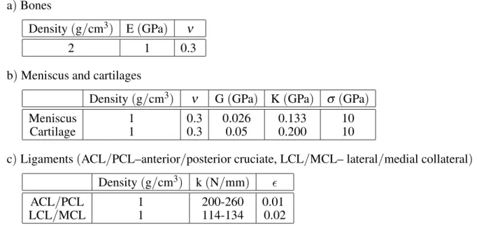
A correct selection of the material and structural properties of knee joint structures is crucial for successful modelling and simulation. It is well known that many of these properties depend on the patient and are also subject to temperature alterations. In this ‘in vivo’ study, the majority of patient-specific parameters could not be mea-sured(e.g. pressure data on the tibia plateau, lig-ament strain), therefore, these parameters were selected from literature. The next simplifica-tion of our model is that all patient properties are the same as in the template. The material and structural properties used in the template
model, gathered in Table 1, are in agreement with the data in(Beillas et al., 2004; Laasanen, 2003).
The described template knee joint model is ac-tually mapped into the patient-specific 3D knee joint FE model as described in subsection 3.1 This process is completely automated, some-times only the bar attachment positions need to be manually fixed/corrected. Figure 4b depicts patient-specific FE model.
Model boundary conditions were estimated from patient-specific data. Several properties of shank and thigh were carefully measured for each pa-tient (e.g. length, diameter, extent). Based on these measurements, a centre of gravity, mass, and three principle moments of inertia were es-timated for bone femur and tibia according to (Zatsiorsky and Seluyanov, 1985). The whole leg was modelled to simulate a patient pushing against the pedal of the MR exercise rig during low-quality imaging. The missing parts of the femur and tibia bones are each modelled by 3 beams attached to the femoral and tibial bone segments. Estimated lengths and masses of the limb segments were used. These beams join in a common node. In the proximal node of the femur beam used to model the hip joint trans-lations are prevented, however, rotations in all directions are allowed. In the distal node of tibia beam used to model the ankle joint only
a)Bones
Density(g/cm3) E(GPa) ν
2 1 0.3
b)Meniscus and cartilages
Density(g/cm3) ν G(GPa) K(GPa) σ (GPa)
Meniscus 1 0.3 0.026 0.133 10
Cartilage 1 0.3 0.05 0.200 10
c)Ligaments(ACL/PCL–anterior/posterior cruciate, LCL/MCL– lateral/medial collateral)
Density(g/cm3) k(N/mm)
ACL/PCL 1 200-260 0.01
LCL/MCL 1 114-134 0.02
Table 1.The material and structural properties of the knee joint structures used in the template knee joint model. Young’s modulus is denoted by E, Poisson’s ratio byν, bulk modulus by K, short time shear modulus by G, yield
rotation in sagittal plane and translation in prox-imal/distal direction are allowed. Both major bones are free in all six degrees of freedom, while the motion of bone patella is restricted to the sagittal plane. The motion of medial/lateral meniscus anterior/posterior horns are free in all six degrees of freedom as well.
3.3. Model of Exercise Rig and Kinematics/Loads
A simple patient knee flexion was simulated by using the described FE model, taking into ac-count the MR scanning procedure at preselected fixed flexions. Accordingly, a model of MR ex-ercise rig with simplified foot-pedal structure was added(see Figure 4c).
The knee joint motion is controlled by several inputs. At the distal node of the tibia bar a compressive load is applied, measured ‘in vivo’ by the force measurement system (see section 2.2). This node is depicted in Figure 4c, where an arrow indicates the direction of the applied concentrated nodal load. Global loads are in-directly determined by the principle moments of inertia calculated for bones femur and tibia. Initial force effect or initial strain value for pre-tensioning is defined for ligaments ACL, LCL, MCL, and deep fibres MCL (see Table 1 for abbreviations). The loads of these element are ranging around 0.04, with the exception of the deep fibres MCL which are set to 0.13. Ap-propriate kinematic response of this model is attained also by suitable setting of linear elas-tic stiffness and mass per unit length of par-ticular element (i.e. ligaments, quadriceps, and hamstrings). To conclude, we see that knee joint is actually modelled as a connected set of strings with single external force applied at the rig pedal. The simulator just seeks an equilib-rium between system’s outer and inner forces.
3.4. Simulation
The developed model simulates flexion of the knee by using an explicit FE code PAM-SAFETM. The following global settings were applied, namely quadratic bulk viscosity coefficient was fixed at 1.2, linear bulk viscosity coefficient was 0.06, hourglass viscosity coefficient was 0.15, and stiffness using elastic modulus was used for
shell hourglass control. The FE simulation was performed in a 300 ms interval, usually finished in around 300 cycles(states). The time interval was 0.01μs and the time step was set to ‘small’. Although our model comprises several knee structures, the motion of the femur bone with respect to the tibia bone was inspected in the present study only. Twenty out-of-plane nodes from each major bone were traced during simu-lation. The following 4×20 matrix was defined at thei-th cycle:
Xi = [ ni,1 ni,2 . . . ni,20 ],
where ni,j = (xi,j,yi,j,zi,j,1) presents coordi-nates for thej-th node. Nodes at cycle 0 deter-mine the initial bone positions. In the sequel, a transformation relative to the straight leg start-ing position was calculated, which was set as the zero flexion position (relative to the static knee flexion of around 10◦). Therefore, the fol-lowing overdetermined linear equation system is solved:
Xi=AiX0,
whereX0 denotes the initial bone position, Xi denotes the bone position at cyclei, andAi
de-notes the affine matrix at cyclei. To capture the motion of the femur bone with respect to the tibia bone, a joint affine matrixJ is calculated ini-th cycle as follows:
Ji=T−i 1Fi,
whereTi and Fidenote affine matrices for the
tibia and femur bones, respectively. Affine ma-trices take the form of:
[R] [L]
0 0 0 1
,
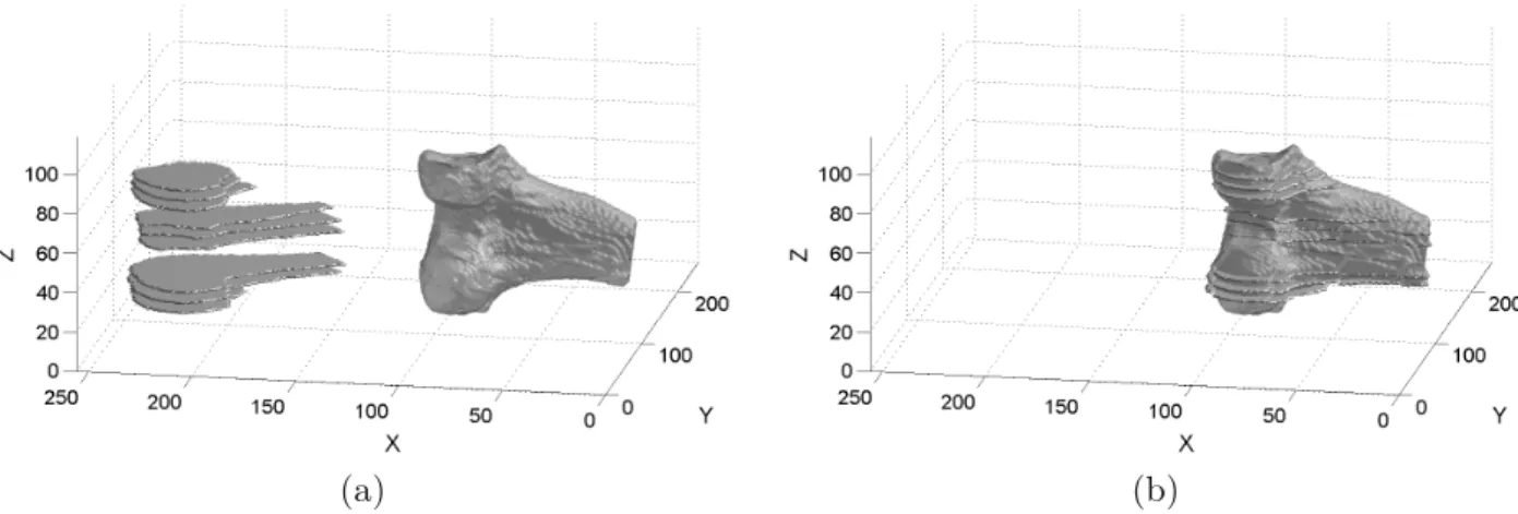
3.5. Evaluation
Simulation results were evaluated against pa-tient imaging data obtained at preselected fixed knee flexions. The idea behind this evaluation is that bones are considered non-deformable structures, and, therefore, their structure and in-terdependence relationship to one another do not change over a short time period. Thus, if the same joint is scanned and reconstructed twice, then both 3D reconstructions must be equal, with just some possible misalignment. Let us present this idea in more detail. A par-tial (sparse) 3D volume is reconstructed from a small number of low-quality images (up to 9 sagittal slices). First, the bones femur and tibia were manually segmented by an expert. These segments were then stacked together to form a partial 3D volume. Sparse 3D volumes were constructed for both major bones at each flexion position(up to 6 flexion positions). Af-terwards, each partial volume is registered to the appropriate 3D volume of the knee joint’s ma-jor bone, reconstructed from the high-quality static imaging data. Figure 5 depicts a rigid registration example of partial 3D volume to the static 3D reconstructed volume for the fe-mur bone. Figure 5a depicts the situation before registration, while(b)depicts rigidly registered volumes. The rigid registration results in an affine transformation matrix. The Euler angles and translations are then calculated as described in subsection 3.4.
4. Results
The simulation of a patient-specific model re-sults in the knee flexion from its initial extended position to the final position of approximately 40◦. The average CPU time required to ac-complish simulation was around 45 hours on a PC-based system with an Intel Pentium Xenon 2.2 GHz processor and 1 GB RAM, where a mesh reconstruction took about 23 minutes and modelling around 1 hour of manual work. It should be noted that the most precise simula-tion with the lowest time step was selected in the PAM-SAFETM. This processing time can easily be reduced by distributed computing (Simbio project, 2003).
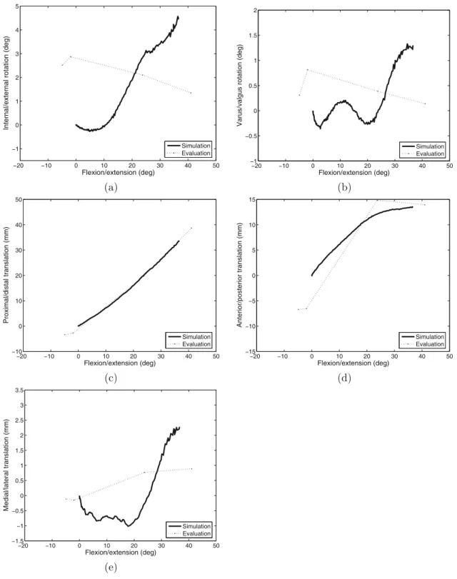
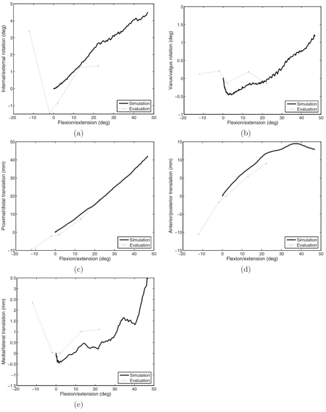
Results for two patients are presented in Fig-ures 6 and 7. Both figFig-ures depict, in bold, the obtained simulation results versus flexion: (a) internal/external rotation,(b)varus/valgus ro-tation,(c)proximal/distal translation,(d) ante-rior/posterior translation, and(e)medial/lateral translation. Evaluation data are represented in the same figures by a dotted line. It should be noted that the first flexion angles (see evalua-tion data)appear as negative angles due to the patients having been scanned at around 10◦ of static flexion. We have to stress again that all Euler angles and translations can only be cal-culated and reported versus flexion angle, sep-arately for the experiment and simulation.
(a) (b)
Ŧ20 Ŧ10 0 10 20 30 40 50
Ŧ1 0 1 2 3 4 5
Flexion/extension (deg)
Internal/external rotation (deg)
Simulation Evaluation
Ŧ20 Ŧ10 0 10 20 30 40 50
Ŧ1
Ŧ0.5 0 0.5 1 1.5 2
Flexion/extension (deg)
Varus/valgus rotation (deg)
Simulation Evaluation
(a) (b)
Ŧ20 Ŧ10 0 10 20 30 40 50
Ŧ10 0 10 20 30 40 50
Flexion/extension (deg)
Proximal/distal translation (mm)
Simulation Evaluation
Ŧ20 Ŧ10 0 10 20 30 40 50
Ŧ15
Ŧ10
Ŧ5 0 5 10 15
Flexion/extension (deg)
Anterior/posterior translation (mm)
Simulation Evaluation
(c) (d)
Ŧ20 Ŧ10 0 10 20 30 40 50
Ŧ1.5
Ŧ1
Ŧ0.5 0 0.5 1 1.5 2 2.5 3 3.5
Flexion/extension (deg)
Medial/lateral translation (mm)
Simulation Evaluation
(e)
Figure 6.Simulation(bold)and experimental(dotted)results for patient A: a)internal/external rotation, b) varus/valgus rotation, c)proximal/distal translation, d)anterior/posterior translation, and e)medial/lateral
translation. Results are depicted versus flexion angle.
A mean square error (MSE) between simula-tion and experimental data was calculated for all patients. The evaluation pointed out that average MSE for the internal/external rota-tion was 1.73◦ (standard deviation std=0.1◦), the average MSE for the varus/valgus rotation
Ŧ20 Ŧ10 0 10 20 30 40 50
Ŧ1 0 1 2 3 4 5
Flexion/extension (deg)
Internal/external rotation (deg)
Simulation Evaluation
Ŧ20 Ŧ10 0 10 20 30 40 50
Ŧ1
Ŧ0.5 0 0.5 1 1.5 2
Flexion/extension (deg)
Varus/valgus rotation (deg)
Simulation Evaluation
(a) (b)
Ŧ20 Ŧ10 0 10 20 30 40 50
Ŧ10 0 10 20 30 40 50
Flexion/extension (deg)
Proximal/distal translation (mm)
Simulation Evaluation
Ŧ20 Ŧ10 0 10 20 30 40 50
Ŧ15
Ŧ10
Ŧ5 0 5 10 15
Flexion/extension (deg)
Anterior/posterior translation (mm)
Simulation Evaluation
(c) (d)
Ŧ20 Ŧ10 0 10 20 30 40 50
Ŧ1.5
Ŧ1
Ŧ0.5 0 0.5 1 1.5 2 2.5 3 3.5
Flexion/extension (deg)
Medial/lateral translation (mm)
Simulation Evaluation
(e)
Figure 7.Simulation(bold)and experimental(dotted)results for patient B: a)internal/external rotation, b) varus/valgus rotation, c)proximal/distal translation, d)anterior/posterior translation, and e)medial/lateral
translation. Results are depicted versus flexion angle.
5. Discussion and conclusions
The aim of this study was to obtain a patient-specific knee joint kinematics during knee flex-ion in controlled environment of the MR scan-ner. Knee flexions from 0◦ to around 40o−
en-vironment makes feasible a credible evaluation of our computer model. Predictions in terms of knee kinematics made by this model were eval-uated against experimentally gathered kinemat-ics data from the preselected fixed knee flexion MR imaging.
Figures 6 and 7 depict the obtained motion of the femur bone with respect to the tibia for two patients. Let us asses the Euler angles first. The simulation results for the varus/valgus rotation, depicted in bold(Figures 6b and 7b), point out a slight increase and, afterwards, stabilization at around 1◦ with the knee flexed by 40◦. In contrast, the varus/valgus used for the evalu-ation (dotted in Figures 6b and 7b) alternates around 0◦. Due to the controlled testing en-vironment, there was practically no rotation in the varus/valgus. The same is evident in the simulation, where the knee joint appears to be relatively stable in varus/valgus(sideways tilt-ing). A similar phenomenon is shown in the internal/external rotation results (see Figures 6a and 7a). Our simulation points out a slight internal rotation from 0◦ to around 4◦ at 40◦ knee flexion. In contrast, the measured data first demonstrates an initial decrease of −10◦, then a slight increase is noticed to around 1◦at 40◦knee flexion. The measured data clearly in-dicates, see Figure 7a, the ‘screw-home’ mech-anism (Moglo and Shirazi-Adl, 2005; Piazza and Cavanagh, 2000)in the first 15◦knee flex-ion (depicted from around −10◦ to around 5◦ knee flexion), thereafter appearing to stabilise around 1◦. In our computer model the initial knee flexion was determined by the angle used in the static MR acquisition; thus the region in which most of the ‘screw-home’ would be likely to occur was not modelled. With regard to trans-lations, a good agreement between the model and measured data is ascertained, especially at proximal/distal translation(see Figures 6c and 7c). In addition, these results point out that the knee joint appears to be relatively stable in me-dial/lateral translation. A bit larger deviation is detected at anterior/posterior translation, how-ever, we notice a similar tendency of simulation and real data(see Figures 6d and 7d). The MR-scanned knee flexions were restricted due to the MR compliant exercise rig, while our model im-poses no extra restrictions. This caused bigger differences between simulation and experiment at large flexion angles.
The accuracy of the final patient-specific model is critical for predicting patient-specific kine-matics. In addition, this accuracy influences also the evaluation procedure (see subsection 3.5). Therefore, a comparison between the template-based automatically constructed pa-tient 3D models and manually created models was carried out. Manual model construction was supervised by orthopaedic surgeons. A dis-parity between two 3D models was calculated in two different ways: a)on slice-to-slice basis by using mean absolute distance (MAD) and b)on surface(volume)basis by using spherical distance(SD). The average MAD calculated for major knee structures is 0.52 mm (std = 0.34 mm), with minimum and maximum being 0.28 mm and 0.75 mm, respectively. On the other side, the average SD is 1.69 mm (std = 3.21 mm), with minimum and maximum being 1.18 mm and 4.91 mm, respectively(Simbio project, 2003; Heric and Potocnik, 2006). From these results we deduce the template matched patient-specific model creation process is of sufficient quality. If gross inaccuracies in the model ap-peared, a manual patient-specific model correc-tion should be applied.
Reference data used in this study were mea-sured non-invasively and without radiation dur-ing controlled experiment. The accuracy of these measurements is influenced by the accu-racy of the 3D reconstruction procedure (see above)and rigid registration method used when aligning sparse fixed-flexion volume with static volume. Efficiency of the applied rigid regis-tration method was tested on artificially gener-ated knee joint data. This assessing pointed out that the applied registration procedure was up to±1◦accurate in rotation and up to±0.2 mm in translation (Simbio project, 2003). From these findings we estimate that the error in our measurement procedure could be in the worst case up to 2◦ by rotation and up to 2 mm by translation. However, it should be emphasized that measurements data were acquired in a con-trolled experiment where this error is essentially smaller.
we found out that obtained patient-specific FE meshes did not provide smooth surface repre-sentations. Surfaces contained so called “ter-racing artefacts”(jagged edges), which resulted from pixelation of the medical imaging data. This problem could be solved only partially by shifting some meshes’ nodes. Namely, smooth object boundaries (surfaces) are highly impor-tant in non-linear FE analyses. For example, to successfully run a simulation where two curved surfaces move over each other, such as is neces-sary for simulating knee joint kinematics, both surfaces must be smooth and without notable discontinuities.
In the sequel, this work is compared to similar, previously published works. A very similar ex-periment was done in(Patel et al., 2004), where the kinematics of constant weight loaded knee during knee flexion from 0◦to 60◦was studied. The work in (Patel et al., 2004) was focused just on motion analysis with no modelling in-cluded. The reported measured knee kinematics is in concordance with our results. The tibial-femoral rotations and translations during knee flexion were also studied in(Moglo and Shirazi-Adl, 2005; Beillas et al., 2004; in Jan et al., 2002 just rotations). Reported results point out a big similarity with our results. In(Beillas et al., 2004), the root mean square errors between computer model and simulation were around 1.4◦ by rotations and around 1 mm by transla-tions, which is in the same quality class as ours (however, for a slightly different experiment). The idea of observing or modelling knee joint kinematics while a knee is slightly loaded is not new. To date, this load is either constant as in (Rothe et al., 2004), or variable according to a predefined function at some intervals as in (Godest et al., 2002). Our approach is different to an extent that ‘in vivo’ acquired load data can be used at the modelling phase. Therefore, a special system was developed for force mea-surements in the magnetic field as explained in subsection 2.2.
Our modelling and knee-kinematics assessment procedure is fully non-invasive, which makes it perfectly suitable for clinical practice. The de-scribed knee joint computer model has not been used in daily clinical practice yet. For such us-age, this model needs to be slightly refined and should undergo more thorough evaluation, e.g. by augmenting the evaluation process by other
major knee joint structures like the patella bone and menisci. The most important research di-rections could be the development of a model for capturing fine kinematics, refining meniscal motion, and study the influences of all patient-specific parameters.
Finally, this model could have a significant im-pact on planning patient-specific operative in-terventions. It could be especially advantageous in situations where postoperative knee joint sta-bility and functionality are not obvious imme-diately.
Acknowledgments
The authors gratefully acknowledge the indis-pensable contributions of Prof. Dr. David Bar-ber, Dr. Steve Wood, and Dr. Avril McCarthy from the Department of Medical Physics and Clinical Engineering, University of Sheffield, England, whose suggestions and help enabled the origins of this work. This work was sup-ported by the European funding within the 5th Framework project entitled ‘SimBio’(Contract No. IST-1999-10378).
References
[1] E. M. ABDEL-RAHMAN, M. S. HEFZY,
Three-dimensional dynamic behaviour of the human knee joint under impact loading.Medical Engineering & Physics, 20(1998), 276–292.
[2] Y. BEI, B. J. FREGLY, Multibody dynamic simulation
of knee contact mechanics.Medical Engineering & Physics, 26(2004), 777–789.
[3] P. BEILLAS, G. PAPAIOANNOU, S. TASHMAN, K. H. YANG, A new method to investigate in-vivo knee behavior using a finite element model of the lower limb.Journal of Biomechanics, 37(2004), 1019– 1030.
[4] T. L. H. DONAHUE, M. L. HULL, M. M. RASHID,
C. R. JACOBS, How the stiffness of meniscal
at-tachments and meniscal material properties affect tibio-femoral contact pressure computed using a validated finite element model of the human knee joint.Journal of Biomechanics, 36(2003), 19–34.
[5] D. DONLAGIC, B. CULSHAW, Propagation of the
[6] M. A. R. FREEMAN, V. PISKERNIKOVA, The
move-ment of the normal tibio-femoral joint.Journal of Biomechanics, 38(2005), 197–208.
[7] W. A. GAMBLING, H. MATSUMURA, C. M. RAG -DALE, R. A. SAMMUT, Measurement of radiation
loss in curved singlemode fibres.Microwaves, op-tics and acousop-tics,2(4) (1978), 134–140.
[8] R. C. GAUTHIER, C. ROSS, Theoretical and exper-imental consideration for single-mode fibre optic bend-type sensors.Applied optics,36(25) (1997), 6264–6273.
[9] A. C. GODEST, M. BEAUGONIN, E. HAUGH, M. TAY -LOR, P. J. GREGSON, Simulation of a knee joint
replacement during a gait cycle using explicit fi-nite element analysis.Journal of Biomechanics, 35 (2002), 267–275.
[10] J. P. HALLORAN, A. J. PETRELLA, P. J. RULLKOET
-TER, Explicit finite element modelling of total knee replacement mechanics.Journal of Biomechanics, 38(2005), 323–331.
[11] D. HERIC, B. POTOCNIK, Objective assessment of
image segmentation algorithms. Electrotechnical Review,74(1-2) (2007), 13–18.
[12] S. V. S. JAN, P. SALVIA, I. HILAL, V. SHOLUKHA, M.
ROOZE, G. CLAPWORTHY, Registration of 6-DOFs electrogoniometry and CT medical imaging for 3D joint modelling.Journal of Biomechanics, 35 (2002), 1475–1484.
[13] M. LAASANEN, Development and validation of
mechano-acoustic techniques and instrument for evaluation of articular cartilage. PhD Thesis,Faculty of Natural and Environmental Sciences, University of Kuopio, 2003.
[14] K. E. MOGLO, A. SHIRAZI-ADL, Cruciate coupling and screw-home mechanism in passive knee joint during extension–flexion.Journal of Biomechanics, 38(5) (2005), 1075–1083.
[15] V. V. PATEL, K. HALL, M. RIES, J. LOTZ, E. OZHIN -SKY, C. LINDSEY, Y. LU, S. MAJUMDAR, A
three-dimensional MRI analysis of knee kinematics. Jour-nal of Orthopaedic Research, 22(2004), 283–292. [16] J. M. T. PENROSE, G. M. HOLT, M. BEAUGONIN,
D. R. HOSE, Developement of an accurate
three-dimensional finite element knee model. Computer Methods in Biomechanics and Biomedical Engi-neering,5(4) (2002), 291–300.
[17] S. J. PIAZZA, P. R. CAVANAGH, Measurement of the
screw-home motion of the knee is sensitive to er-rors in axis alignment.Journal of Biomechanics, 33 (2000), 1029–1034.
[18] B. POTOCNIK, D. HERIC, D. ZAZULA, B. CIGALE,
D. BERNAD, T. TOMAZIˇCˇ, Construction of patient
specific virtual models of medical phenomena. In-formatica,29(2) (2005), 209–218.
[19] W. H. PRESS, S. A. TEUKOLSKY, W. T. VETTERLING,
B. P. FLANNERY,Numerical Recipes in C: The art of
scientific computing. Cambridge University Press, Cambridge, 1992.
[20] R. EISENHART-ROTHE, M. SIEBERT, C. BRINGMANN,
T. VOGL, K.-H. ENGLMEIER, H. GRAICHEN, A new
in-vivo technique for determination of 3D kinemat-ics and contact areas of the patello-femoral and tibio-femoral joint. Journal of Biomechanics, 37 (2004), 927–934.
[21] P. J. ROWE, C. M. MYLES, C. WALKER, R. NUTTON,
Knee joint kinematics in gait and other functional activities measured using flexible electrogoniome-try: how much knee motion is sufficient for normal daily life?.Gait and Posture, 12(2000), 143–155.
[22] N. B. SCHULER, M. J. BEY, J. T. SHEARN, D. L.
BUTLER, Evaluation of an electromagnetic position
tracking device for measuring in-vivo, dynamic joint kinematics.Journal of Biomechanics,38(10) (2005), 2113–2117.
[23] A. B. SHARMA, A.-H. AL-ANI, S. J. HALME,
Constant-curvature loss in monomode fibres: an experimental investigation.Applied optics,23(19) (1984), 3297–3301.
[24] SIMBIO PROJECT, 5th framework programme, no.
IST-1999-10378,http://www.simbio.de, 2003.
[25] V. M. ZATSIORSKY, V. N. SELUYANOV, Estimation
of the mass and inertia characteristics of the human body by means of the best predictive regression equations. InBiomechanics IX-B(D. A. Winter, R. W. Norman, R. P. Wells, K. C. Hayes, A. E. Patla, Ed.),(1985)pp. 233–239.
[26] X. ZHOU, L. F. DRAGANICH, F. AMIROUCHE, A
dy-namic model for simulating a trip and fall during gait. Medical Engineering & Physics, 24 (2002), 121–127.
[27] S. WOOD, D. C. BARBER, A. D. MCCARTHY, D.
CHAN, I. D. WILKINSON, G. DARWENT, D. R. HOSE,
A novel image registration application for the in-vivo quantification of joint kinematics. Presented at theProceedings of Medical Image Understand-ing and Analysis,(2002)University of Portsmouth, Portsmouth.
Received:October, 2007 Revised:May, 2008 Accepted:May, 2008
Contact address: Boˇzidar Potocnikˇ Faculty of Electrical Engineering and Computer Science University of Maribor Smetanova 17, 2000 Maribor, Slovenia Tel.:+386 2 220 74 84 Fax.:+386 2 220 72 72 e-mail:[email protected]
DAMJANZAZULAis a Professor at the Faculty of Electrical Engineering and Computer Science, Maribor. His main research interests are com-pound signal decomposition, biomedical imaging, and virtual training tools.
BORISCIGALEis a teaching assistant at the Faculty of Electrical En-gineering and Computer Science in Maribor. He received his DSc. degree in 2007. His main research interests include image processing of medical images.
DUSANˇ HERICis a teaching assistant at the Faculty of Electrical Engi-neering and Computer Science in Maribor. He received his DSc. degree in 2007. His main research interests are wavelet transformation-adapted analysis and synthesis, active contours, image registration, edge, and contour line detection.
EDVARDCIBULAreceived his Ph.D. degree in electrical engineering from the University of Maribor, Slovenia in 2005. His research interests include fiber optic sensors, smart structures and MOEMS technologies.