Strategic Deployment in Graphs
Elmar Langetepe and Andreas Lenerz
University of Bonn, Department of Computer Science I, Germany
Bernd Brüggemann
FKIE, Fraunhofer-Institute, Germany
Keywords:deployment, networks, optimization, algorithms
Received:June 20, 2014
Conquerors of old (like, e.g., Alexander the Great or Ceasar) had to solve the following deployment prob-lem. Sufficiently strong units had to be stationed at locations of strategic importance, and the moving forces had to be strong enough to advance to the next location. To the best of our knowledge we are the first to consider the (off-line) graph version of this problem. While being NP-hard for general graphs, for trees the minimum number of agents and an optimal deployment can be computed in optimal polynomial time. Moreover, the optimal solution for the minimum spanning tree of an arbitrary graphGresults in a 2-approximation of the optimal solution forG.
Povzetek: Predlagana je izvirna rešitev za razvrstitev enot in premikanje na nove pozicije.
1
Introduction
LetG= (V, E)be a graph with non-negative edge end ver-tex weightsweandwv, respectively. We want to minimize the number of agents needed to traverse the graph subject to the following conditions. If vertex v is visited for the first time,wvagents must be left atvto cover it. An edge
ecan only be traversed by a force of at leastweagents. Fi-nally, all vertices should be covered. All agents start in a predefined start vertexvs ∈ V. In general they can move in different groups. The problem is denoted as astrategic deployment problemofG= (V, E).
The above rules can also easily be interpreted for mod-ern non-military applications. For a given network we would like to rescue or repair the sites (vertices) by a predifined number of agents, whereas traversing along the routes (edges) requires some escorting service. The results presented here can also be applied to a problem of posi-tioning mobile robots for guarding a given terrain; see also [3].
We deal with two variants regarding anotificationat the end of the task. The variants are comparable to routes
(round-trips) andtours(open paths) in traveling-salesman scenarios.
(Return) Finally some agents have to return to the start vertex and report the success of the whole operation.
(No-return) It suffices to fill the vertices as required, no agents have to return to the start vertex.
Reporting the success in the return variant means, that finally a set,M, of agents return tovsand the union ofall
vertices visited by the members ofM equalsV.
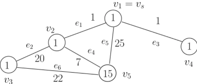
We give an example for the no-return variant for the graph of Figure 1. It is important that the first visit of a
e1
e3
e4
e2
v
1=
v
sv
2v
3v5
v
41
1
1
15
1
1
20
7
1
e5
25
22
e6Figure 1: A graph with edge and vertex weights. If the agents have to start at the vertexv1an optimal deployment strategy
re-quires 23 agents and visits the vertices and edges in a single group in the order (v1,e1,v2,e2,v3,e2,v2,e1,v1,e3,v4,e3,v1,e1,
v2,e4,v5). The traversal fulfills the demand on the vertices in the
orderv1, v2, v3, v4, v5by the first visits w.r.t. the above sequence.
At the end 4 agents are not settled.
vertex immediately binds some units of the agents for the control of the vertex. For start vertexvs = v1 at least 23 agents are required. We let the agents run in a single group. In the beginning one of the agents has to be placed imme-diately inv1. Then we traverse edgee1of weight1 with 22 agents fromv1tov2. Again, we have to place one agent immediately at v2. We move from v2 to v3 along e2 of weight 20 with 21 agents. After leaving one agent atv3we can still move back along edgee2(weight 20) fromv3tov2 with 20 agents. The vertexv2was already covered before. With 20 agents we now visitv4(by traversinge1(weight 1) ande3(weight 1), the vertexv1was already covered and can be passed without loss). We have to place one agent atv4 and proceed with 19 agents alonge3(weight 1),e1 (weight 1) ande4(weight 7) tov5where we finally have to place 15 agents.4agents are not settled.
23 agents. By the results of Section 3 it turns out that the return variant solution has a different visiting order
v1, v2, v3, v5, v4and requires 25 agents.
Although the computation of an efficient flow of some items or goods in a weighted network has a long tra-dition and has been considered under many different aspects the problem presented here cannot be covered by known (multi-agent) routing, network-flow or agent-traversal problems.
For example, in the classical transportation network
problem there are source and sink nodes whose weights represent a supply or a demand, respectively. The weight of an edge represents the transportation cost along the edge. One would like to find a transshipment schedule of mini-mum cost that fulfils the demand of all sink nodes from the source nodes; see for example the monograph of [4] and the textbooks [10, 1] . The solutions of such problems are of-ten based on linear programming methods for minimizing (linear) cost functions.
In apacket routing scenario for a given weighted net-work, m packet sets each consisting of si packets for i = 1,2, . . . mare located at mgiven source nodes. For each packet set a specified sink node is given. Here the edge weights represent anupper boundon the number of single packets that can be transported along the edge in one time step. One is for example interested in minimizing the so-calledmakespan, i.e., the time when the last packet ar-rives at its destination; see for example [13]. For a general overview see also the survey [9].
Similarily, in [11] themulti-robot routingproblem con-siders a set of agents that has to be moved from their start locations to the target locations. For the movement between two locations a cost function is given and the goal is to min-imize the path costs. Such multi-robot routing problems can be considered under many different constraints [16]. For the purpose of patrolling see the survey [14].
Additionally, online multi-agent traversal problems in discrete environments have attracted some attention. The problem of exploring anunknowngraph by a set ofkagents was considered for example in [5, 6]. Exploration means that at the end all vertices of the graph should have been visited. In this motion planning setting either the goal is to optimize the number of overall steps of the agents or to optimize the makespan, that is to minimize the time when the last vertex is visited.
Some other work has been done forkcooperative clean-ers that move around in a grid-graph environment and have toclean each vertex in a contaminated environment; see [2, 17]. In this model the task is different from a simple exploration since after a whilecontaminatedcells can rein-fect cleaned cells. One is searching for strategies for a set ofkagents that guarantee successful cleanings.
Our result shows that finding the minimum number of agents required for the strategic deployment problem is NP-hard for general graphs even if all vertex weights are equal to one. In Section 2 this is shown by a reduction from 3-Exact-Cover (3XC). The optimal number of agents
for the minimum spanning tree (MST) of the graphGgives a2-approximation for the graph itself; see Section 3. For weighted trees we can show that the optimal number of agents and a corresponding strategy forTcan be computed inΘ(nlogn)time. Altogether, a2-approximation forG
can be computed efficiently. Additionally, some structural properties of the problem are given.
The problem definition gives rise to many further inter-esting extensions. For example, here we first consider an offline version with global communication, but also online versions with limited communication might be of some in-terest. Recently, we started to discuss the makespan or traversal time for agiven optimal number of agents. See for example the masterthesis [12] supervised by the second author.
2
General graphs
We consider an edge- and vertex-weighted graph G = (V, E). Letvs∈V denote the start vertex for the traversal of the agents. W.l.o.g. we can assume thatGis connected and does not have multi-edges.
We allow that a traversal strategy subdivides the agents into groups that move separately for a while. A traversal strategy is a schedule for the agents. At any time step any agent decides to move along an outgoing edge of its current vertex towards another vertex or the agent stays in its cur-rent vertex. We assume that any edge can be traversed in one time step.Longconnections can be easily modelled by placing intermediate vertices of weight 0along the edge. Altogether, agent groups can arrive at some vertexvat the same time from different edges.
The schedule is called validif the following condition hold. For the movements during a time step the number of agents that use a single edge has to exceed the edge weight
we. After the movement for any vertexv that already has been visited by some agents, the number of agents that are located atvhas to exceed the vertex weightve. From now on anoptimal deployment strategyis a valid schedule that uses the minimum number of agents required.
Let N := P
v∈V wv denote the number of agents
re-quired for the vertices in total. Obviously, the maximum overall edge weightwmax:= max{we|e∈E}of the graph
gives a simple upper bound for the additional agents (be-yondN) used for edge traversals. This means that at most
wmax+N agents will be required. Withwmax+Nagents
one can for example use a DFS walk along the graph and let the agents run in a single group.
2.1
NP-hardness for general graphs
For showing that computing the optimal number of agents is NP-hard in general we make use of a reduction of the 3-Exact-Cover (3XC) problem. We give the proof for the no-return variant, first.
sub-a
11
1
1
1
1
1
1
1
1
1
1
1
a
2a
3a4
a5
a
6a
7a
8a
9a
10a
11a
12F
1F
2F
3F4
F
5F
6v
sd
1
0
1
1
1
1
1
1
0
0
0
0
0
0
0
m
−
n
+ 1 = 6
−
4 + 1 = 3
3
3
3
3
3
3
3
3
3
3
3
3
3
3
3
3
3
Figure 2: ForX ={a1, a2, . . . , a12}and the subsetsIF = {F1, F2, . . . , F6}withF1 = {a1, a2, a3},F2 = {a1, a2, a4},F3 =
{a3, a5, a7},F4={a5, a8, a9},F5 ={a6, a8, a10}andF6={a9, a11, a12}there is an exact3-cover withF2,F3,F5andF6. For
the start vertexvsan optimal traversal strategy moves in a single group. We start with3n+m+ 1 = 19agents, first visit the vertices
ofF2,F3,F5andF6and cover all elements from there, visiting an element vertex last. After that3n+n= 4n= 16agents have been
placed andm−n+ 1 = 3still have to be placed including the dummy node. With this number of agents we can move back along the corresponding edge of weightm−n+ 1 = 3and place the remaining3agents.
sets ofX so that anyF ∈ IFcontains exactly3elements ofX. The decision problem of 3XC is defined as follows: DoesIFcontain an exact cover ofX of sizen? More pre-cisely is there a subsetFc ⊆ IFso that the collectionFc
contains all elements ofX andFc consists of preciselyn
subsets, i.e. |Fc| = n. It was shown by Karp that this
problem is NP-hard; see Garey and Johnsson[8].
Let us assume that such a problem is given. We de-fine the following deployment problem for (X,IF). Let
X = {a1, a2, . . . , a3n}. For any ai there is an element
vertexv(X)i of weight1. LetIFconsists ofm ≥ n
sub-sets of size3, sayIF ={F1, F2, . . . , Fm}. For anyFj = {aj1, aj2, aj3}we define aset vertexv(IF)jof weight1and
we insert three edges (v(IF)j, v(X)j1), (v(IF)j, v(X)j2) and(v(IF)j, v(X)j3)each of weightm−n+ 1. Addition-ally, we use a sink vertexvsof weightwvs = 0and insert
m edges (vs, v(F)j) from the sink to the set vertices of IF. All these edges get weight0. Additionally, one dummy nodedof weightwd = 1is added as well as an edge(vs, d)
of weight0.
Figure 2 shows an example of the construction for the set X = {a1, a2, . . . , a12} and the subsets IF = {F1, F2, . . . , F6} with F1 = {a1, a2, a3}, F2 = {a1, a2, a4},F3 ={a3, a5, a7},F4 ={a5, a8, a9},F5 = {a6, a8, a10}andF6={a9, a11, a12}withm−n+ 1 = 3. Starting from the sink node vs we are asking whether there is an agent traversal schedule that requires exactly
N = 3n+m+ 1agents. If there is such a traversal this is optimal (we have to fill all vertices). The following result holds.If and only if(X,IF)has an exact3-cover, the given strategic deployment problem can be solved with exactly
N = 3n+m+ 1agents.
Let us first assume that an exact3-cover exists. In this case we start withN = 3n+m+ 1agents atvsand let
the agents run in a single group. First we successively visit the set vertices that build the cover and fill all3nelement vertices using3n+nagents in total. More precisely, for the set vertices that build the cover we successively enter such a vertex from vs, place one agent there and fill all three element vertices by moving back and forth along the corresponding edges. Then we move back tovsand so on. At any such operation the set of agents is reduced by4. Fi-nally, when the last set vertex of the cover was visited, we end in the overall last element vertex. After fulfilling the demand there, we still haveN−4n= 3n+m+ 1−4n= m−n+ 1agents for traveling back tovsalong the cor-responding edges. Now we fill the remaining set vertices by successively moving forth and back fromvsalong the edges of weight0. Finally, with the last agent, we can visit and fill the dummy node.
Conversely, let us assume that there is no exact3-cover for(X,IF)and we would like to solve the strategic deploy-ment problem withN= 3n+m+ 1agents. At some point an optimal solution for the strategic deployment problem has to visit the last element vertexv(X)j, starting from a
set vertexv(IF)i. Let us assume that we are inv(IF)i and
would like to move tov(X)j now andv(X)jwas not
vis-ited before. Since there was no exact3-cover we have al-ready visited strictly more thannset vertices at this point and exactly3n−1element vertices have been visited. This means at least3n−1 +n+ 1 = 4nagents have been used.
Now we consider two cases. If the dummy node was al-ready visited, starting withN agents we only have at most
the last element vertex, this means that we require an ad-ditional agent beyondN for traversing the edge of weight
m−n+ 1. If the dummy node was not visited before and we now decide to move to the last element vertex, we have to place one agent there. This means for travelling back from the last element vertex along some edge (at least the dummy must still be visited), we still require m−n+ 1
agents. Starting withN at the beginning at this stage only
3n+m+ 1−4n−1 = m−nare given. At least one additional agent beyondNis necessary for travelling back to the dummy node for filling this node.
Altogether, we can answer the3-Exact-Cover decision problem by a polynomial reduction into a strategic deploy-ment problem. The proof also works for the return variant, where at least one agent has to return tovs, if we omit the
dummy node, make use ofN := 3n+mand set the non-zero weights tom−n.
Theorem 1. Computing the optimal number of agents for the strategic deployment problem of a general graphGis NP-hard.
2.2
2-approximation by the MST
For a general graphG= (V, E)we consider its minimum spanning tree (MST) and consider an optimal deployment strategy on the MST.
Lemma 1. An optimal deployment strategy for the mini-mum spanning tree (MST) of a weighted graphG= (V, E)
gives a2-approximation of the optimal deployment strategy ofGitself.
Proof: Lete be an edge of the MST of G with maxi-mal weight we among all edges of the MST. It is
sim-ply the nature of the MST, that any traversal of the graph that visits all vertices, has to use an edge of weight at least we. The optimal deployment strategy has to tra-verse an egde of weight at least weand requires at least
kopt ≥max{N, we}agents. The optimal strategy for the
MST approach requires at mostkMST ≤ we+N agents
which giveskMST≤2kopt. 2
2.3
Moving in a single group
In our model it is allowed that the agents run in differ-ent groups. For the computation of the optimal number of agents required, this is not necessary. Note that group-splittingstrategies are necessary for minimizing the com-pletion time. Recently, we also started to discuss such op-timization criteria; see the masterthesis [12] supervised by the first author.
During the execution of the traversal there is a set of set-tledagents that already had to be placed at the visited ver-tices and a set ofnon-settledagents that still move around. We can show that the non-settled agents can always move in a single group. For simplicity we give a proof for trees.
Theorem 2. For a given weighted tree T and the given minimal number of agents required, there is always a de-ployment strategy that lets all non-settled agents move in a single group.
Proof: We can reorganize any optimal strategy accord-ingly, so that the same number of agents is sufficient.
Let us assume that at a vertex v a set of agents X is separated into two groupsX1 andX2and they separately explore disjoint partsT1 and T2 of the tree. LetwTi be the maximum edge weight of the edges traversed by the agentsXi inTi, respectively. Clearly|Xi| ≥ wTi holds. Let|X1| ≥ |X2|hold and letX20 be the set of non-settled agents of X2after the exploration of T2. We can explore
T2byX =X1∪X2agents first, and we do not need the setX2 there. |X1| ≥ wT2 means that we can move back withX1∪X20 agents tovand start the exploration forT1.
The argument can be applied successively for any split of a group. This also means that we can always collect all non-settled vertices in a single moving group. 2 Note that the above Theorem also holds for general graphsG. The general proof requires some technical de-tails because a single vertex might collect agents from dif-ferent sources at the first visit. We omit the rather technical proof here.
Proposition 1. For a given weighted graph G and the given minimal number of agents required, there is always a deployment strategy that lets all non-settled agents move in a single group.
2.4
Counting the number of agents
From now on we only consider strategies where the non-settled agents always move in a single group. Before we proceed, we briefly explain how the number of agents can be computed for a strategy given by a sequenceSof ver-tices and edges that are visited and crossed successively. A pseudocode is given in Algorithm 1. The simple counting procedure will be adapted for Algorithm 2 in Section 3.3 for counting the optimal number of agents efficiently.
For a sequenceS of vertices and edges that are visited and crossed by a single group of agents the required num-ber of agents can be computed as follows. We count the number of additional agents beyond N (where N is the overall sum of the vertex weights) in a variableadd. In an-other variablecurrwe count the number of agents currently available. In the beginningadd := 0andcurr:= N holds. A strategy successively crosses edges and visits vertices of the tree, this is given in the sequenceS. We always choose the next elementx(edgeeor vertexv) out of the sequence. If we would like to cross an edge e, we check whether
curr ≥ we holds. If not we setadd := add+ (we−curr)
Algorithm 1:Number of agents, forG = (V, E)and given sequenceSof vertices and edges.
N :=P
v∈V wv;curr:=N;add:= 0;x:=first(S);
whilex6=NILdo ifxis an edgeethen
ifcurr< wethen
add:=add+ (we−curr);curr:=we; end if
else ifxis a vertexvthen ifcurr< wvthen
add:=add+ (wv−curr);curr:= 0; else
curr:=curr−wv;
end if
wv:= 0;
end if
x:=next(S); end while RETURNN+add
wv := 0, the vertex is filled after the first visit. Obviously this simple algorithm counts the number of agents required in the number of traversal steps of the single group.
3
Optimal solutions for trees
Lemma 1 suggests that for a 2-approximation for a graph
G, we can consider its MST. Thus, it makes sense to solve the problem efficiently for trees. Additionally, by Theorem 1 it suffices to consider strategies of single groups.
vs
n
1 1
0
n−1 · · · 2
1 1 1
Figure 3: An optimal strategy that starts and ends invs has to
visit the leafs with respect to the decreasing order of the edge weights. The minimal number of agents isn+ 1. Any other order will lead to at least one extra agent.
3.1
Computational lower bound
Let us first consider the tree in Figure 3 and the return variant. Obviously it is possible to use n+ 1agents and visit the edges in the decreasing order of the edge weights
n, n−1, . . . ,1. Any other order will increase the number of agents. If for example in the first step an edge of weight
k 6= nis visited, we have to leave one agent at the corre-sponding vertex. Since the edge of weightnstill has to be visited and we have to return to the start,n+ 1agents in total will not be sufficient. So first the edge of weightnhas to be visited. This argument can be applied successively.
Altogether, by the above example there seems to be a computational lower bound for trees with respect to sort-ing the edges by their weights. Since integer values can be sorted by bucket sort in linear time, such a lower bound can only be given for real edge and vertex weights. This seems to be a natural extension of our problem. We con-sider the transportation of sufficient material along an edge (condition 1.). Additionally, the demand of a vertex has to be fully satisfied before transportation can go on (condition 2.). How many material is required?
For a computational lower bound for trees we consider the Uniform-Gap problem. Let us assume thatnunsorted real numbers x1, x2, . . . , xn and an > 0 are given. Is there a permutation π : {1, . . . , n} → {1, . . . , n} so that
xπ(i−1)=xπ(i)+fori= 2, . . . , nholds? In the algebraic decision tree model this problem has computational time boundΩ(nlogn); see for example [15].
In Figure 3 we simply replace the vertex weights of 1
byand thenedge weights byx1, x2, . . . , xn. With the
same arguments as before we conclude: If and only if the Uniform-Gap property holds, a unique optimal strategy has to visit the edges in a single group in the order of decreasing edge weightsxπ(1)> xπ(2)>· · ·> xπ(n)and requires an amount ofxπ(1)+in total. Any other order will lead to at least one extra.
The same arguments can be applied to the no return vari-ant by simple modifications. Only the vertex weight of the smallestxj, sayxπ(n), is set toxπ(n).
Lemma 2. Computing an optimal deployment strategy for a tree of sizenwith positive real edge and vertex weights takesΩ(nlogn)computational time in the algebraic deci-sion tree model.
3.2
Collected subtrees
The proof of Lemma 2 suggests to visit the edges of the tree in the order of decreasing weights. For generalization we introduce the following notations for a treeT with root vertexvs.
For every leaf bl along the unique shortest path, Πbvls, from the root vs tobl there is an edge e(bl)with weight we(bl), so that we(bl)is greater than or equal to any other edge weight alongΠbl
vs. Furthermore, we choosee(bl)so that it has the shortest edge-distance to the root among all edges with the same weight. Let v(bl) denote the vertex of e(bl) that is closer to the leafbl. Thus, every leaf bl
defines a unique path, Tbl, fromv(bl)to the leafbl with incoming edge e(bl)with edge weight we(bl). The edge
e(bl)dominatesthe leafbland also the pathT(bl).
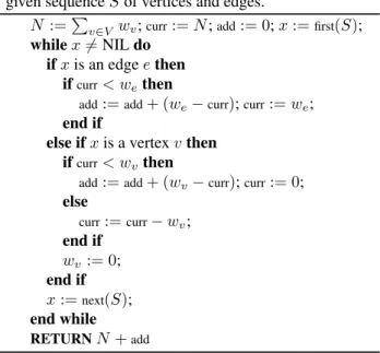
For example in Figure 4 we havee(b2) =e5andv(b2) =
v3, the pathT(b2)fromv3 overv5tob2is dominated by the edgee5of weight10.
If some pathsTbl
For example, in Figure 4 forb6andb7we havev(b6) =
v(b7) =v4ande(b6) =e(b7) =e7andT(b6, b7)is given by the treeTv4that is dominated by edgee7.
Altogether, for any treeT there is a unique set of disjoint collected subtrees (a path is a subtree as well) as uniquely defined above and we can sort them by the weight of its dominating edge. For the tree in Figure 4 we have disjoint subtreesT(b6, b7),T(b2, b3, b4),T(b1),T(b5)andT(b0) in this order.
e1
e11 e10
v3
b4 1
3 10
3 8
e4
e2
v1
b0 b1
5
2 3
4 9
vs 4
e9 e8
v2
b6 b7
5
2 1
1 3
e5
b5 2
9 6
v4
e3 e6
12 e7 7 2
e13 e12
v5
b2 b3
1
2 1
2 1
T(b0) T(b1)
T(b2, b3, b4)
T(b5)
T(b6, b7)
Figure 4: The optimal strategy with start and end vertexvs
vis-its, fully explores and leaves the collected subtrees T(b6, b7),
T(b2, b3, b4),T(b1),T(b5)andT(b0)in the order of the weights
we7 = 12,we5 = 10,we3 = 9,we4 = 7andwe2 = 4of the dominating edges.
3.3
Return variant for trees
We show that the collected subtrees can be visited in the order of the dominating edges.
Theorem 3. An optimal deployment strategy that has to start and end at the same root vertexvsof a treeTcan visit the disjoint subtreesT(bl1, bl2, . . . , blm)in the decreasing
order of the dominating edges.
Any tree T(bl1, bl2, . . . , blm) can be visited, fully
ex-plored in some order (for example by DFS) and left then. An optimal visiting order of the leafs and the optimal number of agents required can be computed inΘ(nlogn)
time for real edge and vertex weights and in optimalΘ(n)
time for integer weights.
For the proof of the above Theorem we first show that we can reorganize any optimal strategy so that at first the tree
T(bl1, bl2, . . . , blm)with maximal dominating edge weight can be visited, fully explored and left, if the strategy does not end in this subtree (which is always true for the return variant). The number of agents required cannot increase. This argument can be applied successively. Therefore we formulate the statement in a more general fashion.
Lemma 3. Let T(bl1, bl2, . . . , blm) be a subtree that is dominated by an edge e which has the greatest weight among all edges that dominate a subtree.
LetSbe an optimal deployment strategy that visits some vertex vt last and let vt be not a vertex inside the tree T(bl1, bl2, . . . , Tblm). The strategyS can be reorganized
so that first the treeT(bl1, bl2, . . . , blm)can be visited, fully
explored in any order and finally left then.
Proof: The treeT(bl1, bl2, . . . , Tblm)rooted atv(bl1)and with maximal dominating edge weight we(bl1) does not contain another subtreeT(bk1, bk2, . . . , Tbkn). This means that T(bl1, bl2, . . . , Tblm)is the full subtree Tv(bl1) of T rooted at v(bl1). Let Path(v(bl1) denote the number of agents that has to be settled along the unique path from
vsto the predecessor,pred(v(bl1)), ofv(bl1).
Let us assume that an optimal strategy is given by a sequence S and let Sv(i) denote the strategy that ends after the i-th visit of some vertex v in the sequence of
S. Let |Sv(i)| denote the number of settled agents and let curr(Sv(i)) denote the number of non-settled agents after the i-th visit of v. We would like to replace S
by a sequence S0S00. If vertex v(bl1) is finally vis-ited, say for the k-th time, in the sequence S, we re-quire curr(Sv(bl1)(k)) ≥ we(bl1) and |Sv(bl1)(k)| ≥ |T(bl1, bl2, . . . , Tblm)|+Path(v(bl1)since the strategy ends atvt6∈T(bl1, bl2, . . . , Tblm). In the next stepSwill move back topred(v(bl1))alonge(bl1)and inSthe rootv(bl1)of the treeT(bl1, bl2, . . . , Tblm)and the edgee(bl1)will never be visited again.
If we consider a strategy S0 that first visits v(bl1), fully explores T(bl1, bl2, . . . , Tblm) by DFS and moves back to the start vs by passing e(bl1), the minimal number of agents required for this move-ment is exactly |T(bl1, bl2, . . . , Tblm)| + Path(v(bl1) + we(bl1) with we(bl1) non-settled agents. With
|Sv(bl1)| − |T(bl1, bl2, . . . , Tblm)| −Path(v(bl1)
+ we(bl1)agents we now start the whole sequenceSagain.
In the concatenation of S0 and S, say S0S, the vertex v(bl1) is visited k
0 = k + 2 times for
|T(bl1, bl2, . . . , Tblm)| ≥2andk
0=k+1times form= 1
andv(bl1) =T(bl1, bl2, . . . , Tblm).
After S0 was executed for the remaining move-ment of S0Sv(bl1)(k
0) the portion w
e(bl1) of
|Sv(bl1)| − |T(bl1, bl2, . . . , Tblm)| −Path(v(bl1)
+ we(bl1) allows us to cross all edges in S
0S
v(bl1)(k
0) for free, becausewe(bl1)is the maximal weight in the tree.
Thus obviously curr(S0Sv(bl1)(k
0)) = curr(Sv
(bl1)(k)) holds andS0S andS require the same number of agents.
In S0S all visits ofT(b
l1, bl2, . . . , Tblm)made byS were useless because the tree was already completely filled by
S0. Skipping all these visits inS, we obtain a sequenceS00
subtree T(bl1, bl2, . . . , blm)contains the vertexvs visited last. Let us assume thatN1is the optimal number of agents required forT.
After the first application of Lemma 3 to the subtree
T(bl1, bl2, . . . , blm) with greatest incoming edge weight
we(bl1)we can move with at least we(bl1)agents back to the rootvswithout loss by the strategyS0. Let us assume thatN10 agents return to the start.
We simple set all node weights along the path from
vs to v(bl1) to zero, cut off the fully explored sub-tree T(bl1, bl2, . . . , blm) and obtain a tree T0. Note that the collected subtrees were disjoint and apart from
T(bl1, bl2, . . . , blm) the remaining collected subtrees will be the same in T0 and T. By induction on the number of the subtrees in the remainingproblemT0 we can visit
the collected subtrees in the order of the dominating edge weights.
Note that the number of agents required forT0might be less thanN10because the weightwe(bl1)was responsible for
N10. This makes no difference in the argumentation. We consider the running time. By a simple DFS walk of T, we compute the disjoint trees T(bl1, bl2, . . . , blm)
implicitly by pointers to the root vertices v(bl1). For any vertex v, there is a pointer to its unique subtree
T(bl1, bl2, . . . , blm) and we compute the sum of the ver-tex weights for any subtree. This can be done in overall linear time. Finally, we can sort the trees by the order of the weights of the incoming edges inO(nlogn)time for real weights and inO(n)time for integer weights.
For computing the number of agents required, we make use of the following efficient procedure, similar to the al-gorithm indicated at the beginning of this Section. Any vis-ited vertex will be marked. In the beginning letadd:= 0and
curr:=N. Let|T(bl1, bl2, . . . , blm)|denote the sum of the vertex weights of the corresponding tree. We successively
jumpto the verticesv(bl1)of the treesT(bl1, bl2, . . . , blm) by making use of the pointers. We markv(bl1)and starting with the predecessor ofv(bl1)we move backwards along the path from v(bl1)to the rootvs, until the first marked vertex is found. Unmarked vertices along this path are la-beled as marked and the sum of the corresponding vertex weights is counted in a variablePath. Additionally, for any such vertexvthat belongs to some other subtreeT(. . .)we subtract the vertex weight wv from|T(. . .)|, this part of
T(. . .)is already visited.
Now we setcurr:=curr−(|T(bl1, bl2, . . . , blm)|+Path). If curr < weholds, we set add := add+ (we−curr)and
curr := we as before. Then we turn over to the next tree. Obviously with this procedure we compute the optimal number of agents in linear time, any vertex is marked only once. A pseudocode is presented in Algorithm 2. 2 We present an example of the execution of Algorithm 2. For example in Figure 4 we haveN := 41and first jump to the rootv4ofT(b6, b7), we have|T(b6, b7)|= 8. Then we count the 6agents along the path from v4 back tovs and mark the vertices v2 and vs as visited. This gives
curr:= 41−(8 + 6) = 27, which is greater thanwe7 = 12.
Additionally, forv2we subtract2from|T(b5)|which gives |T(b5)|= 9. Now we jump to the rootv3ofT(b2, b3, b4) with|T(b2, b3, b4)| = 8. Moving fromv3 back tovsto
the first unmarked vertex just gives no step. No agents are counted along this path. Thereforecurr:= 27−(8+0) = 19
andcurr> we5 = 10. Next we jump to the rootb1ofT(b1) of size|T(b1)|= 3. Moving back to the root we count the weight5of the unvisited vertexv1(which will be marked now). Note that v1 does not belong to a subtreeT(. . .). We havecurr := 19−(3 + 5) = 11. Now we jump to the rootv2ofT(b5)of current size|T(b5)|= 9. Therefore
curr:= 11−(9+0) = 2which is now smaller thanwe4 = 7. This givesadd := add+ (we−curr) = 0 + (7−2) = 5
and curr := we = 7. Finally we jump to b0 = T(b0) and have curr := 7−(2−0) = 5 which is greater than
we2. Altogether 5 additional agent can move back tovs andN+add= 46agents are required in total.
Algorithm 2: Return variant. Number of agents for
T = (V, E). Rootsv(bl1)of treesT(bl1, bl2, . . . , blm)
are given by pointers in a listLin the order of dom-inating edge weights. NIL is the predecessor of root
vs.
N :=P
v∈V wv;curr:=N;add:= 0;
whileL6=∅do
v(bl1) :=first(L);deleteFirst(L); Markv(bl1);
Path:= 0;pathv:=pred(v(bl1));
whilepathvnot marked andpathv6=NILdo
Path:=Path+wpathv;
ifpathvbelongs toT(. . .)then |T(. . .)|:=|T(. . .)| −wpathv
end if
Markpathv;pathv:=pred(pathv); end while
curr:=curr−(|T(bl1, bl2, . . . , blm)|+Path). ifcurr< wethen
add:=add+ (we−curr);curr:=we; end if
end while RETURNN+add
3.4
Lower bound for traversal steps
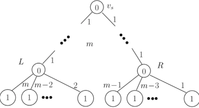
It is easy to see that although the number of agents required and the visiting order of the leafs can be computed sub-quadratic optimal time, the number of traversal steps for a tree could be inΩ(n2); see the example in Figure 5. In this example the strategy with the minimal number of agents is unique and the agents have to run in a single group.
3.5
No-return variant
1 1 1 1 1 1
m m−2 2 m−1 m−3 1
0
0
0
vs
m
L 1 1 R
1 1
Figure 5: An optimal deployment strategy for the tree with3m
edges requiresm+ 1agents and successively moves fromLtoR
beyondvsin totalΩ m2
times. ThusΩ(m2)steps are required.
subtrees will be visited in the order of the decreasing dom-inating edge weights.
For example a strategy for the no-return in Figure 4 that visits the collected subtreesT(b6, b7),T(b2, b3, b4),T(b1),
T(b5)and T(b0) in the order of the weightswe7 = 12,
we5 = 10,we3 = 9,we4 = 7andwe2= 4of the dominat-ing edges requires46agents even if we do not finally move back to the start vertex. As shown at the end of Section 3.3 we required5additional agents for leavingT(b5), entering and leavingT(b0)afterwards requires no more additional agents.
In the no return variant, we can assume that any strategy ends in a leaf, because the last vertex that will be served has to be a leaf. This also means that it is reasonable to enter a collected subtree, which will not be left any more. In the example above we simply change the order of the last two subtrees. If we enter the collected subtrees in the order
T(b6, b7),T(b2, b3, b4),T(b1),T(b0)andT(b5)andT(b5) is not left at the end, we end the strategy inb5(no-return) and require exactlyN = 41agents, which is optimal.
Theorem 4. For a weighted treeT with given rootvsand
non-fixed end vertex we can compute an optimal visiting or-der of the leafs and the number of agents required in amor-tized timeO(nlogn).
For the proof of the above statement we first characterize the structure of an optimal strategy. Obviously we can as-sume that a strategy that need not return to the start will end in a leaf. Let us first assume that the final leaf,bt, is already
known or given. As indicated for the example above, the
finalcollected subtree will break the order of the collected subtrees in an optimal solution. This behaviour holds re-cursively.
Lemma 4. An optimal traversal strategy that has to visit the leaf bt last can be computed as follows: Let T(bl1, bl2, . . . , blm)be the collected subtree ofT that
con-tainsbt.
1. First, all collected subtrees T(bq1, bq2, . . . , bqo) of the treeT with dominating edge weight greater than
T(bl1, bl2, . . . , blm)are successively visited and fully
explored (each by DFS) and left in the decreasing or-der of the weights of the dominating edges.
2. Then, the remaining collected subtrees that do not contain bt are visited in an arbitrary order (for
ex-ample by DFS).
3. Finally, the collected subtreeT(bl1, bl2, . . . , blm)that containsbtis visited. Here we recursively apply the same strategy to the subtreeT(bl1, bl2, . . . , blm). That is, we build a list of collected subtrees for the tree
T(bl1, bl2, . . . , blm)and recursively visit the collected subtrees by steps 1. and 2. so that the collected sub-tree that containsbtis recursively visited last in step 3. again.
Proof: The precondition of the Theorem says that there is an optimal strategy given by a sequence S of visited vertices and edges so that the strategy ends in the leafbt.
LetT(bl1, bl2, . . . , blm)be the collected subtree ofT that containsbtand letwe(bt)be the corresponding dominating edge weight. Sobt ∈ {bl1, bl2, . . . , blm}andv(bt)is the root of T(bl1, bl2, . . . , blm). Similarily as in the proof of Lemma 3 we would like to reorganizeSas required in the Lemma.
For the treesT(bq1, bq2, . . . , bqo)with dominating edge weight greater than we(bt) we can successively apply Lemma 3. So we reorganizeSis this way by a sequenceS0
that finally moves the agents back to the start vertex vs. Then we apply the sequence S again but skip the visits of all collected subtrees already fully visited byS0before.
This show step 1. of the Theorem.
This gives an overall sequenceS0S00with the same num-ber of agents andS00 does only visit collected subtrees of
T with dominating edges weight smaller than or equal to
we(bt). Furthermore,S00also ends inbt.
The collected subtree T(bl1, bl2, . . . , blm) with weight
we(bt)does not contain any collected subtree with weight smaller than or equal towe(bt). At some point inS00the ver-texv(bt)is visited for the last time, say for thek-th time, by a movement from the predecessorpred(v(bt)ofv(bt)by passing the edge of weightwe(bt). At leastwe(bt) agents are still required for this step. At this moment all subtrees different fromT(bl1, bl2, . . . , blm)and edge weight smaller than or equal towe(bt)habe been visited since the strategy ends inbt∈ {bl1, bl2, . . . , blm}.
Sincewe(bt)agents are required for the final movement along e(bt) there will be no loss of agents, if we
pos-tone all movements intoT(bl1, bl2, . . . , blm)inS
00first and
then finally solve the problem inT(bl1, bl2, . . . , blm) opti-mally. For the subtrees different fromT(bl1, bl2, . . . , blm)
and edge weight smaller than or equal towe(bt)we only re-quire the agents that have to be placed there, since at least
we(bt) non-settled agents will be always present. There-fore we can also decide to visit the subtrees different from
Finally, we arrive atv(bt)andT(bl1, bl2, . . . , blm)and would like to end in the leafbt. By induction on the height of the trees the treeT(bl1, bl2, . . . , blm)can be handled in the same way. That is, we build a list of collected subtrees for the treeT(bl1, bl2, . . . , blm)itself and recursively visit the collected subtrees by steps 1. and 2. so that the col-lected subtree that containsbtis recursively visited last in
step 3. again. 2
The remaining task is to efficiently find the best leafbt
where the overall optimal strategy ends. The above Lemma states that we should be able to start the algorithm recur-sively at the root of a collected subtreeT(bl1, bl2, . . . , blm) that containsbt. Forvsa list,L, of the collected subtrees
forT is given and for finding an optimal strategy we have to compute the corresponding lists of collected subtrees for all treesT(bl1, bl2, . . . , blm)inLrecursively.
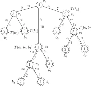
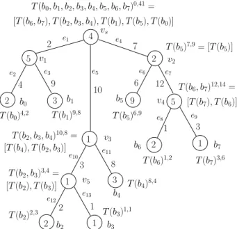
Figure 6 shows an example. In this setting let us for example consider the case that we would like to compute an optimal visiting order so that the strategy has to end in the leaf b2. Since b2 is in T(b2, b3, b4) in the list of vs in Figure 6 by the above Lemma in step 1. we first visit the treeT(b6, b7)of dominating edge weight greater than the dominating edge weight ofT(b2, b3, b4). Then we visit
T(b1),T(b5)andT(b0)in step 2. After that in step 3. we recursively start the algorithm inT(b2, b3, b4). Here atv3 the list of collected sutrees contains T(b4) andT(b2, b3) and by the above recursive algorithm in step 1. we first visitT(b4). There is no tree for step 2. and we recursively enterT(b2, b3)atv5in step 3. Here for step 1. there is no subtree and we enter the treeT(b3)in step 2. until finally we recursively end inT(b2)in step 3. Here the algorithm ends. Note that in this exampleb2is not the overall optimal final leaf.
If we simply apply the given algorithm for any leaf and compare the given results (number of agents required) we requireO(n2logn)computational time. For efficiency, we compute the required information in a single step and check the value for the different leafs successively. It can be shown that in such a way the best leafbt and the overall optimal strategy can be computed in amortizedO(nlogn)
time.
Finally, we give a proof for Theorem 4 by the fol-lowing discussion. We would like to compute the lists of the collected subtrees T(bl1, bl2, . . . , blm) recur-sively. More precisely, for the root vs of a full tree T with leafs {b1, b2, . . . , bn} we obtain a list, denoted by T(b1, b2, . . . , bn), of the collected subtrees of T with respect to the decreasing order of the dominating edge weights as introduced in Section 3.2.
The elements of the list are pointers to the roots of the collected subtreesT(bl1, bl2, . . . , blm). For any such root
T(bl1, bl2, . . . , blm)of a subtree in the listT(b1, b2, . . . , br) we recursively would like to compute the corresponding list of collected subtrees recursively; see Figure 6 for an example.
Additionally, for any considered collected subtree
T(bk1, bk2, . . . , bkr) that belongs to the pointer list of
e1
e11 e10
v3
b4 1
3 10
3 8
e4
e2
v1
b0 b1
5
2 3
4 9
vs 4
e9 e8
v2
b6 b7
5
2 1
1 3
e5
b5 2
9 6
v4
e3 e6
12 e7 7 2
e13 e12
v5
b2 b3
1
2 1
2 1
T(b0)4,2 T(b1)9,8
T(b2, b3, b4)10,8=
T(b5)6,9
T(b6, b7)12,14=
T(b2)2,3 T(b3) 1,1 T(b2, b3)3,4=
T(b4)8,4
T(b6)1,2 T(b7)3,6 [T(b7), T(b6)] [T(b6, b7), T(b2, b3, b4), T(b1), T(b5), T(b0)]
[T(b4), T(b2, b3)]
[T(b2), T(b3)]
T(b0, b1, b2, b3, b4, b5, b6, b7)0,41=
T(b5)7,9= [T(b5)]
Figure 6: All information required can be computed recursively from bottom to top in amortizedO(nlogn)time.
T(bl1, bl2, . . . , blm) we store a pair of integers x, y at the corresponding root of T(bk1, bk2, . . . , bkr); see Fig-ure 6. Herexdenotes the weight of the dominating edge. The value y denotes the size of |T(bk1, bk2, . . . , bkr)|+
Path), if we recursively start the optimal tree algorithm in the root T(bl1, bl2, . . . , blm); see Algorithm 2. This means that y denotes the size of the collected sub-tree and the sum of the weights along the path back fromT(bk1, bk2, . . . , bkr)to the rootT(bl1, bl2, . . . , blm)if
T(bk1, bk2, . . . , bkr), ifT(bk1, bk2, . . . , bkr)is the first en-try of the listT(bl1, bl2, . . . , blm)and therefore has maxi-mal weight.
The list of subtrees at the root vs of T is denoted by
T(b1, b2, . . . , br)x,y and obtains the valuesx:= 0(no in-coming edge) and y := N (the sum of the overall vertex weights). We can show that all information can be com-puted efficiently from bottom to top and finally also allows us to compute an overall optimal strategy.
For the overall construction of all pointer lists
T(bl1, bl2, . . . , blm) we internally make use of Fibonacci heaps [7]. The corresponding heap for a vertexv always containsallcollected subtrees of the leafs ofTv. The col-lected subtree list for the vertexvitself might be empty; see for example that vertexv1does not root a set of collected subtree. In the following the list of pointers to collected subtrees is denoted by[. . .]and the internal heaps are de-noted by(. . .).
or-der) have the same elements.
With the help of the heaps we successively compute and store the final collected subtree lists for the vertices. We start the computations on the leafs of the tree. For a single leaf bl the heap(T(bl)x,y) and the subtreeT(bl)x,y
rep-resent exactly the same. The valuexofT(bl)x,y is given
by the edge weight of the leaf. The value y of T(bl)x,y
will be computed recursively, it is initialized by the vertex weight of the leaf. For example, in Figure 6 forb7andb6 we first haveT(b6)1,2andT(b7)3,1, representing both the heaps and the subtrees.
Let us assume that the heaps for the child nodes of an internal node v already have been computed and v is a branching vertex with incoming edge weightwe. We have to add the node weight ofvto the valueyof one of the sub-trees in the heap. We simply additionally store the subtree with greatest weight among the branches. Thus in constant tim we add the node weight of the branching vertex to the valuey of a subtree with greatest weight. Then we unify the heaps of the children. They are given in theincreasing
order of the dominating edges weights. This can be done in time proportional to the number of child nodes ofv. For example, atv4in Figure 6 first we increase they-element of the subtreeT(b7)3,1 in the heap by the vertex weight5 ofv4which givesT(b7)3,6. Then we unify(T(b6)1,2)and (T(b7)3,6)to a heap(T(b6)1,2, T(b7)3,6). For convenience in the heap we attach the values x andy directly to the pointer of the subtree.
Now, for branching vertex v by using the new unified heap we find, delete and collect the subtrees with minimal incoming edge weight as long as the weights are smaller than or equal to the weightwe. If there is no such tree, we
do not have to build a new collected subtree at this vertex and also the heap remains unchanged. If there are some subtrees that have incoming edge weight smaller than or equal to we the pointers to all these subtrees will build a new collected subtreeT(bl1, bl2, . . . , blm)withx-valuewe
at the nodev. Additionally, the pointers to the correspond-ing subtrees of T(bl1, bl2, . . . , blm)can easily be ordered withincreasingweights since we have deleted them out of the heap starting with the smallest weights. Additionally, we sum up the valuesyof the deleted subtrees. Finally, we have computed the collected subtree T(bl1, bl2, . . . , blm)
and its informationx, yat nodev. At the end a new subtree is also inserted into the fibonacci heap of the vertexv for future unions and computations.
For example in Figure 6 for the just computed heap
(T(b6)1,2, T(b7)3,6)at vertexv4we delete and collect the subtreesT(b6)1,2andT(b7)3,6out of the heap because the weightwe7 = 12 dominates both weights1and3. This gives a new subtree T(b7, b6)12,8 = [T(b7), T(b6)]atv4 and also a heap(T(b7, b6)12,8).
Note, that sometimes no new subtree is build if no tree is deleted out of the heap because the weight of the incoming edge is less than the current weights. Or it might happen that only a single tree of the heap is collected and gets a new dominating edge. In this case also no subtree is deleted out
of the heap. We have a single subtree with the same leafs as before but with a different dominating edge. We do not build a a collected subtree for the vertex at this moment, the insertion of such subtrees at the corresponding vertex is postponed.
For example for the vertex v2 with incoming edge weight 7 in Figure 6 we have already computed the heaps(T(b5)6,9)and(T(b6, b7)12,8)of the subtrees. Now the vertex weight 2 of v2 is added to the y-value of
T(b6, b7)12,8 which givesT(b6, b7)12,10 for this subtree. Then we unify the heaps to (T(b5)6,9, T(b6, b7)12,10). Now with respect to the incoming edges weight7only the first tree in the heap is collected to a subtree and this subtree gives the list for vertexv2. The heap of the vertexv2now reads(T(b5)7,9, T(b7, b6)12,10)and the collected subtree is
T(b5)7,9= [T(b5)].
Finally, we arrive the root vertexvsand all subtrees of
the heap are inserted into the list of collected subtrees for the root.
The delete operation for the heaps requires amortized
O(logm) time for a heap of size m and subsumes any other operation. Any delete operation leads to a collection of subtrees, therefore at most O(n)delete operation will occur. Altogether all subtrees and its pointer lists and the valuesxandy can be computed in amortizedO(nlogn)
time.
The remaining task is that we use the information of the subtrees for calculating the optimal visiting order of the leafs in overallO(nlogn)time. Here Algorithm 2 will be used as a subroutine.
As already mentioned we only have to fix the leafbt vis-ited last. We proceed as follows. An optimal strategy ends in a given collected subtree with some dominating edge weightwe. The strategy visits and explores the remaining
trees in the order of the dominating edges weights. Let us assume that on the top level the collected sub-trees are ordered by the weights we1 ≤ we2 ≤ . . . ≤
wej. Therefore by the given information and with Algo-rithm 2 for anyi we can successively compute the num-ber of additional agents required for any successive order
wei+1 ≤wei+2 ≤. . . ≤ wej and by they-values we can also compute the number of agents required for the trees of the weightswe1 ≤ we2 ≤ . . . ≤ wei−1. The number of agents required for the final tree of weightweiand the best final leaf stems from recursion. With this informations the number of agents can be computed. This can be done in overall linear timeO(j)for anyi.
The overall number of collected subtrees in the construc-tion is linear for the following reason. We start withn sub-trees at the leafs. If this subtree appears again in some list (not in the heap), either it has been collected together with some others or it builds a subtree for its own (changing dominance of a single tree). If it was collected, it will never appear for its own again on the path to the root. If it is a single subtree of that node, no other subtree appears in the list at this node. Thus for theO(n)nodes we haveO(n)
From i to i+ 1only a constant number of additional calculations have to be made. By induction this can recur-sively be done for the subtree dominated by wei as well. Therefore we can use the given information for computing the optimal strategy in overall linear timeO(n)if the col-lected subtrees are given recursively.
4
Conclusion
We introduce a novel traversal problem in weighted graphs that models security or occupation constraints and gives rise to many further extensions and modifications. The problem discussed here is NP-hard in general and can be solved efficiently for trees inΘ(nlogn)where some ma-chinery is necessary. This also gives a2-approximation for a general graph by the MST.
References
[1] R. K. Ahuja, T. L. Magnanti, and J. B. Orlin. Net-work Flows: Theory, Algorithms, and Applications. Prentice Hall, Englewood Cliffs, NJ, 1993.
[2] Th. Beckmann, R. Klein, D. Kriesel, and E. Langetepe. Ant-sweep: a decentral strategy for cooperative cleaning in expanding domains. In Symposium on Computational Geometry, pages 287–288, 2011.
[3] Bernd Brüggemann, Elmar Langetepe, Andreas Lenerz, and Dirk Schulz. From a multi-robot global plan to single-robot actions. InICINCO (2), pages 419–422, 2012.
[4] V. Chvátal. Linear Programming. W. H. Freeman, New York, NY, 1983.
[5] M. Dynia, J. Łopusza´nski, and Ch. Schindelhauer. Why robots need maps. InSIROCCO ’07: Proc. 14th Colloq. on Structural Information an Communication Complexity, LNCS, pages 37–46. Springer, 2007.
[6] P. Fraigniaud, L. Gasieniec, D. R. Kowalski, and A. Pelc. Collective tree exploration. Networks, 43(3):166–177, 2006.
[7] M. L. Fredman and R. E. Tarjan. Fibonacci heaps and their uses in improved network optimization al-gorithms.J. ACM, 34:596–615, 1987.
[8] M. R. Garey and D. S. Johnson. Computers and Intractability: A Guide to the Theory of NP-Completeness. W. H. Freeman, New York, NY, 1979.
[9] Miltos D. Grammatikakis, D. Frank Hsu, Miro Kraetzl, and Jop F. Sibeyn. Packet routing in fixed-connection networks: A survey. Journal of Parallel and Distributed Computing, 54(2):77 – 132, 1998.
[10] Bernhard Korte and Jens Vygen. Combinatorial Op-timization: Theory and Algorithms. Springer Publish-ing Company, Incorporated, 4th edition, 2007.
[11] Michail G. Lagoudakis, Evangelos Markakis, David Kempe, Pinar Keskinocak, Anton Kleywegt, Sven Koenig, Craig Tovey, Adam Meyerson, and Sonal Jain. Auction-based multi-robot routing. In Proceed-ings of Robotics: Science and Systems, Cambridge, USA, June 2005.
[12] Simone Lehmann. Graphtraversierungen mit Nebenbedingungen. Masterthesis, Rheinische Friedrich-Wilhelms-Universität Bonn, 2012.
[13] Britta Peis, Martin Skutella, and Andreas Wiese. Packet routing: Complexity and algorithms. In
WAOA 2009, number 5893 in LNCS, pages 217–228. Springer-Verlag, 2009.
[14] David Portugal and Rui P. Rocha. A survey on multi-robot patrolling algorithms. In Luis M. Camarinha-Matos, editor, DoCEIS, volume 349 of IFIP Ad-vances in Information and Communication Technol-ogy, pages 139–146. Springer, 2011.
[15] F. P. Preparata and M. I. Shamos.Computational Ge-ometry: An Introduction. Springer-Verlag, New York, NY, 1985.
[16] Alexander V. Sadovsky, Damek Davis, and Dou-glas R. Isaacson. Optimal routing and control of multiple agents moving in a transportation network and subject to an arrival schedule and separation con-straints. InNo. NASA/TM–2012–216032, 2010.