Total Least Squares Fitting the Three-Parameter Inverse Weibull Density

Vol. 7, No. 3, 2014, 230-245

ISSN 1307-5543 – www.ejpam.com

Total Least Squares Fitting the Three-Parameter Inverse Weibull

Density

Dragan Juki´c, Darija Markovi´c

Department of Mathematics, J.J. Strossmayer University of Osijek, Trg Ljudevita Gaja 6, HR-31 000 Osijek, Croatia

Abstract. The focus of this paper is on a nonlinear weighted total least squares fitting problem for the three-parameter inverse Weibull density which is frequently employed as a model in reliability and lifetime studies. As a main result, a theorem on the existence of the total least squares estimator is obtained, as well as its generalization in thel_qnorm (1_≤q<_∞).

2010 Mathematics Subject Classifications: 65D10, 62J02, 62G07, 62N05

Key Words and Phrases: inverse Weibull density, total least squares, total least squares estimate, existence problem, data fitting

1. Introduction

The probability density function of the random variableThaving a three-parameter inverse Weibull distribution (IWD) with location parameterα_≥0, scale parameterη >0 and shape parameterβ >0 is given by

f(t;α,β,η) =

(

β η

η

t−α

β+1_e−( η t−α)

β

t> α

0 t≤α. (1)

If α= 0, the resulting distribution is called the two-parameter inverse Weibull distribution. This model was developed by Erto[6].

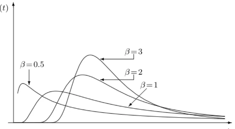
The IWD is very flexible and by an appropriate choice of the shape parameterβ the den-sity curve can assume a wide variety of shapes (see Fig. 1). The denden-sity function is strictly increasing on (α,tm] and strictly decreasing on [tm,∞), where tm = α+η(1+1/β)−1/β. This implies that the density function is unimodal with the maximum value att_m. This is in contrast to the standard Weibull model where the shape is either decreasing (for β ≤ 1) or unimodal (forβ >1). Whenβ = 1, the IWD becomes an inverse exponential distribution;

∗_{Corresponding author.}

Email addresses:[email protected](D. Juki´c),[email protected](D. Markovi´c)

whenβ=2, it is identical to the inverse Rayleigh distribution; whenβ=0.5, it approximates the inverse Gamma distribution. That is the reason why the IWD is a frequently used model in reliability and lifetime studies (see e.g. Cohen and Whitten [5], Lawles [18], Murthy et al.[21], Nelson[22]).

t f(t) ✻

✲ β= 0.5

❄

β= 3 ✛

β= 2 ✛

β= 1

✠

Figure 1: Plots of the inverse Weibull density for some values ofβand by assumingα=0 and η=1.2

In practice, the unknown parameters α, β andηof the three-parameter inverse Weibull density (1) are not known in advance and must be estimated from a random samplet₁, . . . ,tn consisting ofnobservations of the three-parameter inverse Weibull random variableT. There is no unique way to estimate the unknown parameters and many different methods have been proposed in the literature (see e.g. Abbasiet al.[1], Lawless[18], Maruši´cet al.[20], Murthyet al. [21], Nelson[22], Silverman[26], Smith and Naylor[27, 28], Tapia and Thompson[29]).

A very popular method for parameter estimation is the least squares method. The non-linear weighted ordinary least squares (OLS) fitting problem for the three-parameter inverse Weibull density is considered by Maruši´cet al. [20]. In this paper we consider the

nonlin-ear weighted total least squares (TLS) fitting problem for the three-parameter inverse Weibull density function. The structure of the paper is as follows. In Section 2 we briefly describe the TLS method and present our main result (Theorem 1) which guarantees the existence of the TLS estimator for the three-parametric inverse Weibull density. Its generalization in thel_q norm (1_≤q<_∞) is given in Theorem 2. All proofs are given in Section 3.

2. The TLS Fitting Problem for the Three-parameter Inverse Weibull Density

Both the OLS and the TLS method require the initial nonparametric density estimates ˆf which need to be as good as possible (see e.g. Silverman[26], Maruši´cet al.[20]). Suppose

we are given the points(ti,yi),i=1, . . . ,n,n>3, where 0<t₁<t₂<. . .<t_n

The goal of the OLS method (see e.g. [2, 3, 8, 11, 13, 14, 19, 25]) is to choose the unknown

parameters of density function (1) such that the weighted sum of squared distances between the model and the data is as small as possible. To be more precise, let w_i > 0, i= 1, . . . ,n, be the data weights which describe the assumed relative accuracy of the data. The unknown parametersα,β andηhave to be estimated by minimizing the functional

S(α,β,η) = n X

i=1

wi[f(ti;α,β,η)− yi]2

on the set

P :=(α,β,η)_∈R3:α_≥0;β,η >0 .

A point (α⋆,β⋆,η⋆) ∈ P such that S(α⋆,β⋆,η⋆) = inf_{(α,β,η)∈P} S(α,β,η) is called the OLS estimator, if it exists. As we have already mentioned, this problem has been solved by Maruši´c et al.[20].

In the OLS approach the observations t_i of the independent variable are assumed to be exact and only the estimates y_i of the density (dependent variable) are subject to random errors. Unfortunately, this assumption does not seem to be very realistic in practice, and many errors (sampling errors, human errors, modeling errors and instrument errors) prevent us from knowing t_i exactly. In such situation, when also the observations of the independent variable contains errors, it seems reasonable to estimate the unknown parameters so that the weighted sum of squares of all errors is minimized. This approach, known as the total least squares (TLS) method, is a natural generalization of the OLS method (see e.g. [7]). In the statistics

literature, the TLS approach is known aserrors-in-variables regression ororthogonal distance regression, and in numerical analysis it was first considered by Golub and Van Loan[9].

The TLS method can be described as follows. Letw_i,p_i>0,i=1, . . . ,n, be some weights. If we assume that yi contains unknown additive error ǫi and that ti has unknown additive errorδ_i, then the mathematical model becomes

y_i= f(t_i+δ_i;α,β,η) +ǫ_i, i=1, . . . ,n.

The unknown parameters α,β andη of density function (1) have to be estimated by mini-mizing the weighted sum of squares of all errors, i.e. by minimini-mizing the functional (see e.g.

[4, 7, 10, 17, 24])

T(α,β,η,δ) = n X

i=1

wi[f(ti+δi;α,β,η)−yi]2+ n X

i=1

piδ2i (2)

on the setP ×Rn. A point_(α⋆,_β⋆,_η⋆₎inP is called the_{total least squares estimator}(TLS

es-timator) of the unknown parameters(α,β,η)for the three-parameter inverse Weibull density, if there existsδ⋆∈Rnsuch that

T(α⋆,β⋆,η⋆,δ⋆_{) =} inf

(α,β,η,δ)_{∈P ×}RnT(α,β,η,

δ₎.

Numerical methods for solving the nonlinear TLS problem are described in Boggs et al.

minimization of the sum of squares it is still necessary to ask whether the TLS estimator exists. In the case of nonlinear TLS problems it is still extremely difficult to answer this question (see e.g.[3, 7, 12, 15–17]).

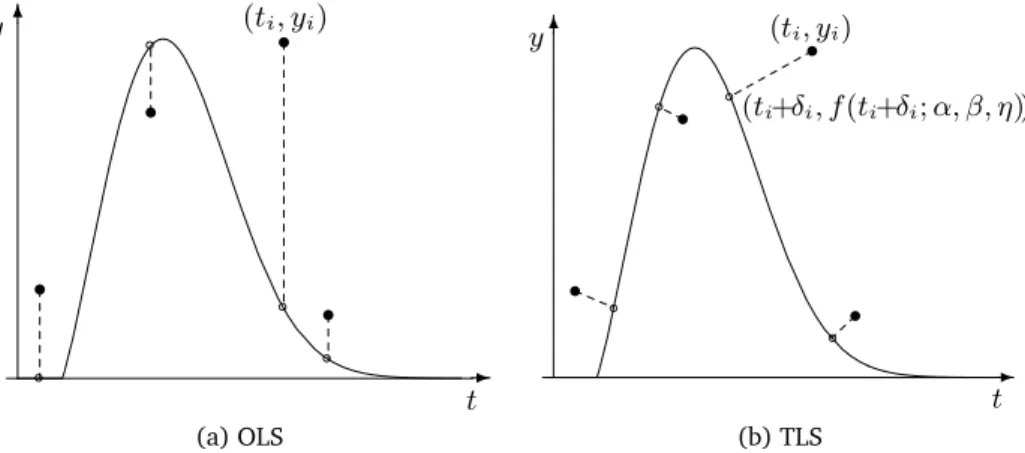
The difference between the OLS and the TLS approach is illustrated in Fig. 2. Geometri-cally, ifw_i=p_i for alli=1, . . . ,n, minimization of functionalT corresponds to minimization of the weighted sum of squares of distances from data points to the model curve.

(ti, yi)

❛

❛

❛

❛

t y ✻

✲

(a) OLS

(ti, yi)

❛ ❛

❛

❛

t

y ✻

✲ (ti+δi, f(ti+δi;α, β, η))

(b) TLS

Figure 2: The difference between the OLS and TLS approaches

Our main existence result for the TLS problem for the three-parameter inverse Weibull density is given in the next theorem.

Theorem 1. Let the points(t_i,y_i), i=1, . . . ,n, n>3, be given, such that0<t₁<t₂<. . .<t_n and yi >0, i=1, . . . ,n. Furthermore, let wi,pi >0, i =1, . . . ,n, be some weights. Then there exists a point(α⋆,β⋆,η⋆,δ⋆₎∈ P ×Rn _{such that}

T(α⋆,β⋆,η⋆,δ⋆) = inf

(α,β,η,δ)∈P ×RnT(α,β,η,

δ),

i.e. the TLS estimator exists.

The proof is given in Section 3. The following total l_q norm (q _≥ 1) generalization of Theorem 1 holds true.

Theorem 2. Suppose1 ≤ q < _∞. Let the points and weights be the same as in Theorem 1. Define

T_q(α,β,η,δ₎:₌ n X

i=1

w_if(t_i+δ_i;α,β,η)−y_i q

+ n X

i=1

p_i|δ_i|q. (3)

Then there exists a point(α⋆_q,β_q⋆,η⋆_q,δ⋆

q)∈ P ×R

n _{such that}

Tq(α⋆q,β

⋆

q,η

⋆

q,δ

⋆

q) =_(α,β,η,inf_{δ)∈P ×R}nTq(α,β,η,

δ).

3. Proof of Theorem 1

Before starting the proof of Theorem 1, we need some preliminary results. Lemma 1. Suppose we are given data(w_i,t_i,y_i), i∈I:={1, . . . ,n}, n>3, such that

0<t₁ <t₂<. . .<t_n and y_i >0, i_∈I . Let w_i,p_i >0, i_∈I , be some weights. Given any real number q,1≤q<_∞, and any nonempty subset I₀of I , let

Σ_I0:= X i∈I\I0

w_iy_iq+X i∈I0

p_i|t_i−τ₀|q,

where

τ₀∈argmin x

n X

i=1

p_i|t_i−x|q.

Then there exists a point inP ×Rn_{at which functional Tqdefined by}(3)_{attains a value less than}

Σ_I0.

Summation P i∈I0

is to be understood as follows: The sum over those indicesi≤nfor which i ∈ I₀. If there are no such indices, the sum is empty; following the usual convention, we define it to be zero. Summation P

i∈I\I0

has similar meanings.

It is easy to verify that t₁≤mini∈I0ti ≤τ0≤maxi∈I0ti ≤tn. Note that for the case when

q = 2,τ₀ is a well known weighted arithmetic mean, and for the case whenq =1, τ₀ is a weighted median of the data (see e.g. Sabo and Scitovski[23]).

Proof. Sinceτ₀ is an element of the closed interval[t₁,tn], there existsr ∈ {1, . . . ,n}such that

τ₀∈(t_r−1,t_r],

where t₀=0 by definition. Let us first choose real y₀such that 0< y₀<min

i∈I yi (4)

and then define functionsα,β,η:(0, 1)_→Rby:

β(b):=τ₀y₀e b

b η(b):=τ₀b1/β(b),

α(b):=τ₀₋η(b)b−1/2β(b)=η(b)b−1/β(b)−b−1/2β(b). Clearly, functionsβ andηare positive. Furthermore, by using the inequality

b−1/β(b)−b−1/2β(b)>0, which holds for everyb∈(0, 1), it is easy to show that functionαis also positive. Thus, we have showed that(α(b),β(b),η(b))_{∈ P} for all b∈(0, 1). Let us now associate with each realb∈(0, 1)a three-parametric inverse Weibull density function

f(t;α(β),β(b),η(b)) =

 



β(b)

t−α(b)

η(b)

t−α(b)

β(b)

e− t−η(αb()b)

β(b)

t> α(b)

0 t≤α(b).

This function has maximum at the point

α(b) +η(b)(1+1/β(b))−1/β(b)=τ₀₋ǫ(b), where

ǫ(b):=η(b)”b−1/2β(b)−€1+ 1 β(b)

Š−1/β(b)— .

It is strictly increasing on(α(b),τ₀−ǫ(b)]and strictly decreasing on[τ₀−ǫ(b),∞). Further-more, by a straightforward calculation, it can be verified that

f(τ₀+α(b);α(b),β(b),η(b)) = y₀, (6) lim

b→0β(b) =∞, (7)

lim

b→0η(b) =τ0, (8)

lim

b→0α(b) =0. (9)

Now we are going to show that

lim

b→0f(t;α(b),β(b),η(b)) =0, t6=τ0. (10) First, in view of (8) and (9), we obtain

lim b→0

€ η(b) t−α(b)

Š

= τ0 t .

Ifτ₀<t, then from (7) and (9) it follows readily that lim_b→0e−

η(b) t−α(b)

β(b)

=1 and limb→0β(b)

€ _η(b) t−α(b)

Šβ(b)

=0, and therefore

lim

b→0f(t;α(b),β(b),η(b)) =blim→0

” β(b) t−α(b)

€ η(b) t−α(b)

Šβ(b)

e− t−η(αb()b)

β(b)

—

=0.

Ifτ₀>t, then there exists a sufficiently greatk₀∈Nsuch that

e<€ η(b) t−α(b)

Šk0

for every sufficiently smallb>0. Now, by using the inequality x<ex (x ≥0) we obtain

β(b)<eβ(b)<€ η(b) t−α(b)

Šk0β(b)

, b≈0,

and therefore, for any b≈0 we have

0<f(t;α(b),β(b),η(b)) = β(b) t−α(b)

€ η(b) t−α(b)

Šβ(b)

e− η(b) t−α(b)

< 1 t−α(b)

€ η(b) t−α(b)

Š(k0+1)β(b)

e− t−ηα(b()b)

β(b)

.

Since

lim b→0

€ η(b) t−α(b)

Š(k0+1)β(b)

e− η(b) t−α(b)

β(b)

=0, then from the above-mentioned inequality it follows that

lim

b→0f(t;α(b),β(b),η(b)) =0, t> τ0. Thus, we proved the desired limits (10).

Note that

f(τ₀;α(b),β(b),η(b)) = β(b) τ₀−α(b)

€ η(b) τ₀−α(b)

Šβ(b)

e− τ₀η−(αb)(b)

β(b)

= β(b) τ₀₋α(b)

p be−

p

b₌ τ0y0eb−

p

b

(τ₀₋α(b))pb, from where taking the limit asb→0 it follows that

lim

b→0f(τ0;α(b),β(b),η(b)) =∞. (11) Due to (9), (10) and (11), we may suppose that bis sufficiently small, so that

0< α(b)<t₁ (12) 0< f(t_i;α(b),β(b),η(b))< y_i, if t_i 6=τ₀ (13)

f(τ₀;α(b),β(b),η(b))>max

i∈I yi. (14)

Let us now show that for eachi∈I₀and for everyb∈(0, 1)there exists a unique number τ_i(b)such that (see Figure 3)

  

 

t_i < τ_i(b)< τ₀−ǫ(b)< τ₀, ift_i< τ₀ ti < τi(b)<ti+ǫ(b), ifti=τ0 τ₀< τ_i(b)<t_i, ift_i> τ₀

(15)

and

f(τ_i(b);α(b),β(b),η(b)) = y_i. (16) First, since the function t 7→ f(t_i;α(b),β(b),η(b))has maximum at the pointτ₀−ǫ(b)and it is strictly increasing on(α(b),τ₀−ǫ(b)]and strictly decreasing on[τ₀−ǫ(b),∞), by using (4), (6), (13) and (14) we obtain

  

 

The existence of the desired numbersτ_i(b),i∈I₀, follows from the well-known Intermediate Value Theorem which states that a continuous real function assumes all intermediate values on a closed interval, while uniqueness follows from monotonicity.

t f(t) ✻

✲

τ0₋ε(b) τ0 τ0+ε(b) ❝

s

s

(tj, yj)

(τj(b), yj) ❝ s

s ❝

(ti, yi) (τi(b), yi) s

Figure 3: i,j ∈ I₀, t_i < τ₀, t_j > τ₀; 0 < δ_i(b) = τ_i(b)− t_i < τ₀−ǫ(b)−t_i < τ₀− t_i; τ₀₋t_j< τ_j(b)₋t_j=δ_j(b)<0

Setting

δ_i(b):=

¨

τ_i(b)−t_i, ifi∈I₀

0, if i∈I\I₀, (17)

(16) becomes

f(t_i+δ_i(b);α(b),β(b),η(b)) = y_i, i∈I₀. (18) Note that only one of the following two cases can occur:

(i) _|I₀|=1, or (ii) _|I₀|>1.

Case(i): |I₀|=1. In this case we haveτ₀= t_r. It follows from (15) that 0< δ_r(b)< ǫ(b). Without loss of generality, in addition to (12)-(14) we may suppose thatbis sufficiently small, so that

tr−1+ǫ(b)<

t_r−1+t_r

2 <tr−ǫ(b) and

f((t_r−1+t_r)/2;α(b),β(b),η(b))<min i∈I yi.

Ift_i<t_r, then

0<f(t_i;α(b)−δ_r(b),β(b),η(b)) = f(t_i+δ_r(b);α(b),β(b),η(b)) <f(t_i+ǫ(b);α(b),β(b),η(b))_≤ f(t_r−1+ǫ(b);α(b),β(b),η(b)) <f((tr−1+tr)/2;α(b),β(b),η(b))<min

i∈I yi ≤ yi, (19)

whereas if ti>tr, then

0<f(ti;α(b)−δr(b),β(b),η(b)) = f(ti+δr(b);α(b),β(b),η(b))

<f(t_i;α(b),β(b),η(b))< y_i. (20) Thus, it follows from (18), (19) and (20) that, for every b∈(0, 1),

T_q(α(b)−δ_r(b),β(b),η(b),0) = n X

i=1

w_if(t_i;α(b)−δ_r(b),β(b),η(b))−y_i q

< n X

i=1 i6=r

wiy q i = ΣI0

Case|I₀|>1. Note that only one of the following two subcases can occur: (i) τ₀₆=ti for alli∈I0, or

(ii) τ₀=tr for somer∈I0.

Subcase(i): In this subcase, it follows from (13), (15), (17) and (18) that, for everyb∈(0, 1), T_q(α(b),β(b),η(b),δ_{(b)) =} X

i∈I\I0

w_if(t_i;α(b),β(b),η(b))−y_i q+

X

i∈I0

p_i|δ_i(b)|q

< X i∈I\I0

wiy q i +

X

i∈I0

pi|ti−τ0|q= ΣI0.

Subcase(ii): Assume thatτ₀=t_rfor somer∈I₀. Let indexs∈I₀be such thatt_s< τ₀. Then by (15), for everyb∈(0, 1),

0< δ_r(b)< ǫ(b)and 0< δ_s(b)<tr−ǫ(b)−ts and therefore

p_s|δ_s(b)_|q+p_r|δ_r(b)_|q<p_s|t_r−ǫ(b)₋t_s|q+p_rǫq(b). It can be easily shown that the above right-hand side is less than

ps|tr−ts|q

wheneverbis small enough. Therefore, for every small enoughbwe have

Tq(α(b),β(b),η(b),δ(b)) = X

i∈I\I0

wi

+p_r|δ_r(b)|q+p_s|δ_s(b)|q+ X i∈I0\{r,s}

p_i|δ_i(b)|q

< X i∈I\I0

w_iy_iq+X i∈I0

p_i|t_i−τ₀|q= Σ_I0.

This completes the proof of the lemma.

Proof of Theorem 1.

Proof. Since functional T is nonnegative, there exists T⋆:= inf

(α,β,η,δ)∈P ×RnT(α,β,η,

δ).

To complete the proof it should be shown that there exists a point(α⋆,β⋆,η⋆,δ⋆₎∈ P ×Rn

such thatT(α⋆,β⋆,η⋆,δ⋆_{) =T}⋆.

Let(α_k,β_k,η_k,δk)be a sequence in_{P ×}Rn, such that

T⋆= lim

k→∞T(αk,βk,ηk,

δk_{) =} lim k→∞

” X

i∈I

w_i f(t_i+δ_ik;α_k,β_k,η_k)−y_i2+X i∈I

p_i(δ_ik)2

= lim k→∞

¦ X

ti+δik≤αk

w_iy_i2+ X

ti+δik>αk

w_i”βk η_k

€ η

k ti+δk_i −αk

Šβk+1

e−

η_k

ti+δk i−αk

β_k −y_i—2

+X i∈I

pi(δki) 2©

. (21)

whereI={1, . . . ,n}. The summation P ti+δik≤αk

(or P

ti+δik>αk

) is to be understood as follows: The

sum over those indices i≤nfor which ti+δki ≤αk (or ti+δik > αk). If there are no such pointst_i, the sum is empty; following the usual convention, we define it to be zero.

There is no loss of generality in assuming that all sequences(α_k),(β_k),(η_k),(δk₁), . . . ,(δ_nk) are monotone. This is possible because the sequence (α_k,β_k,η_k,δ₁k, . . . ,δk_n) has a subse-quence (α_l

k,βlk,ηlk,δ

lk

1, . . . ,δ lk

n), such that all its component sequences are monotone; and since limk→∞T(αlk,βlk,ηlk,δ

lk_{) =}lim

k→∞T(αk,βk,ηk,δk) =T⋆.

Since each monotone sequence of real numbers converges in the extended real number system ¯R, define

α⋆:= lim

k→∞αk, β

⋆_{:= lim}

k→∞βk, η

⋆_{:= lim}

k→∞ηk, δ

⋆_{:= lim}

k→∞δ

k_{= (δ}⋆

1, . . . ,δ⋆n). Note that 0 ≤ α⋆,β⋆,η⋆ ≤ ∞, because (α_k,β_k,η_k) ∈ P. Also note thatδ⋆_i ∈ R for each

i =1, . . . ,n. Indeed, if_|δ⋆_i|=_∞for some i, then it would follow from (21) that T⋆= _∞, which is impossible.

To complete the proof it is enough to show that(α⋆,β⋆,η⋆)∈ P, i.e. that

It remains to show that(α⋆,β⋆,η⋆)∈ P. The proof will be done in five steps. In step 1 we will show thatα⋆< t_n. In step 2 we will show thatβ⋆₆=0. The proof thatη⋆ ₆=_∞will be done in step 3. In step 4 we prove thatη⋆₆=0. Finally, in step 5 we show thatβ⋆₆=_∞.

Step 1. Ifα⋆_≥t_n, from (21) it follows thatT⋆=Pn_i=1w_iy_i2+P_i∈Ip_iδ⋆_i2. Since according to Lemma 1 (forq=2 andI₀=_{1_}) there exists a point in_{P ×}Rnat which functional_T attains

a value smaller thanΣ_I0and sinceΣ_I0<Pn_i=1wiyi2+ P

i∈Ipiδ⋆

2

i , this means that in this way (α⋆_≥t

n) functional T cannot attain its infimum. Thus, we have proved thatα⋆<tn.

Before continuing the proof, let us introduce some notation and make one remark. First let us define

I₀:=

¨

I_α⋆, ifI_α⋆ 6=; {1_}, otherwise where Iα⋆ :={i∈I:t_i+δ⋆

i =α

⋆_{}. Let us note that Lemma 1 withq=2 implies that}

T⋆< X i∈I\I0

w_iy_i2+X i∈I0

p_i(t_i−τ_I0)2=:Σ_I0, (22)

whereτ_I0=

P

i∈I₀piti

P

i∈I₀pi .

By taking an appropriate subsequence of(α_k,β_k,η_k,δk₎, if necessary, we may assume that if ti+δ⋆i < α

⋆_{, then t}

i+δki < αk for everyk∈N. Similarly, if ti+δ⋆i > α

⋆_{, we may assume}

that ti+δki > αkfor everyk∈N. Due to this, now it is easy to show that from (21) it follows that

T⋆≥ X ti+δ⋆i<α⋆

w_iy_i2+ lim k→∞

¦ X

ti+δ⋆i>α⋆

w_i”βk η_k

€ η

k ti+δik−αk

Šβk+1

e−

η_k

ti+δk i−αk

β_k

−y_i—2©

+X i∈I

piδ⋆

2

i . (23)

Step 2. Ifβ⋆=0, then by using the inequalityx <ex _{(x≥0) we obtain}

0< βk η_k

€ η_k

t_i+δk i −αk

Šβk+1

e−

η_k

ti+δk i−αk

β_k

< βk t_i+δk

i −αk

, if ti+δ⋆i > α

⋆_,

wherefrom it follows readily that

lim k→∞ ”β k η_k € η k ti+δ_ik−αk

Šβk+1

e−

η_k

ti+δk i−αk

β_k

—

=0, if t_i+δ⋆_i > α⋆.

Now, from (23) it follows that

T⋆≥ X

i∈I\I0

wiyi2+ X

i∈I0

piδ⋆

2

= X i∈I\I0

w_iy_i2+X i∈I0

p_i(t_i−α⋆)2

≥ X

i∈I\I0

w_iy_i2+X i∈I0

p_i(t_i−τ_I0)2= Σ_I0, (24)

which contradicts (22). Therefore, in this way (β⋆_{=0) functionalTcannot attain its infimum.}

Thus, we have proved thatβ⋆₆=0.

The last inequality in (24) follows directly from a well-known fact that the quadratic func-tion x7→P_i∈I

0pi(ti−x)

2_{attains its minimum}P

i∈I0pi(ti−τI0)

2_{at pointτ} I0.

Step 3. Let us show thatη⋆₆=_∞. We prove this by contradiction. Suppose on the contrary that η⋆ = ∞. Without loss of generality, we may then assume that if t_i+δ⋆_i > α⋆, then e< ηk

ti+δki−αk for allk∈

N. Then from the inequality_x<ex(x _≥0) it follows that ifti+δ⋆i > α

⋆_,

then

β_k<eβk _<

€ η_k

t_i+δk_i −α_k Šβk

, k∈N.

Thus, ift_i+δ⋆_i > α⋆, then

0<βk η_k

€ η_k

t_i+δk i −αk

Šβk+1

e−

η_k

ti+δk i−αk

β_k

= βk t_i+δk

i −αk

€ η_k

t_i+δk i −αk

Šβk

e−

η_k

ti+δk i−αk

β_k

< 1 t_i+δk

i −αk

€ η_k

t_i+δk i −αk

Š2βk

e−

η_k

ti+δk i−αk

β_k

. (25)

Furthermore, since limk→∞ ti+δηkik−αk

=∞andβ⋆6=0, we have lim_k→∞ ηk

ti+δki−αk

βk

=∞

and therefore lim_k→∞ ηk

ti+δki−αk

2βk_e− η_k

ti+δk i−αk

β_k

=0, so that from (25) it follows that

lim k→∞

”β_k η_k

€ η_k

t_i+δ_ik−α_k Šβk+1

e−

η_k

ti+δk i−αk

β_k

—

=0, if ti+δ⋆i > α

⋆_.

Putting the above limits into (23), we immediately obtain

T⋆≥ X

i∈I\I0

w_iy_i2+

X

i∈I

p_iδ⋆_i2≥Σ_I0,

which contradicts (22). Hence we proved thatη⋆6=∞.

So far we have shown thatα⋆< tn,β⋆6=0 andη⋆ 6=∞. By using this, in the next step we will show thatη⋆₆=0.

(i) η⋆=0 andβ⋆∈(0,∞), or (ii) η⋆=0 andβ⋆=_∞.

Now, we are going to show that functionalT cannot attain its infimum in either of these two cases, which will prove thatη⋆6=0.

Case(i): η⋆=0 andβ⋆∈(0,∞). In this case we would have

lim k→∞

β_k η_k

€ η_k

t_i+δk i −αk

Šβk+1

e−

η_k

ti+δk i−αk

β_k

= lim k→∞

β_k t_i+δk

i −αk

€ η_k

t_i+δk i −αk

Šβk

e−

η_k

ti+δk i−αk

β_k

=0, ift_i+δ⋆_i > α⋆ and hence from (23) it would follow that

T⋆_≥ X ti+δ⋆i6=α⋆

w_iy_i2+X i∈I

p_iδ⋆_i2_≥Σ_I0

which contradicts assumption (22).

Case(ii): η⋆=0 andβ⋆=∞. Sinceη_k→0, there exists a real numberL>1 and sufficiently greatk_0∈Nsuch that if_ti+δ⋆

i > α

⋆_andk>k

0, thenηk/(ti+δik−αk)<1/L. Without loss of generality, we may assume thatk₀=1. Thus, ifti+δ⋆i > α

⋆_{, then}

0<βk η_k

€ η

k ti+δik−αk

Šβk+1

e−

η_k

ti+δk i−αk

β_k

= βk ti+δki −αk

€ η

k ti+δki −αk

Šβk

e−

η_k

ti+δk i−αk

β_k

< 1 ti+δik−αk

€β k Lβk

Š e−

η_k

ti+δk i−αk

β_k

. (26)

Furthermore, since

lim k→∞

€β_k Lβk

Š

=0 and lim k→∞e

− ηk ti+δk

i−αk

β_k

=1, from (26) it follows that

lim k→∞

”β_k η_k

€ η_k

ti+δik−αk Šβk+1

e−

η_k

ti+δk i−αk

β_k

—

=0, if t_i+δ⋆_i > α⋆.

Finally, from (23) we obtain T⋆≥ P_t

i+δ⋆i6=α⋆wiy

2 i +

P i∈Ipiδ⋆

2

i ≥ ΣI0, which contradicts

Step 5. It remains to show that β⋆ 6= ∞. We prove this by contradiction. Suppose that β⋆=_∞. Arguing as in case (ii) from step 4, it can be shown that

lim k→∞

” β_k

t_i+δk_i −α_k

€ η_k

t_i+δ_ik−α_k Šβk

e−

η_k

ti+δk i−αk

β_k

—

=0, if 0< η

⋆

ti+δ⋆_i −α⋆

<1. (27)

If η⋆

ti+δ⋆i−α⋆

>1, then there exists a sufficiently greatk₀ ∈N such that e< ηk

ti+δik−αk

k0_{. Now,}

by using the inequality x<ex (x ≥0) we obtain

β_k<eβk _<

€ η

k ti+δ_ik−αk

Šk0βk

, k_∈N,

and therefore

0< βk ti+δk_i −αk

€ η

k ti+δ_ik−αk

Šβk

e−

η_k

ti+δk i−αk

β_k

< 1 ti+δk_i −αk

€ η

k ti+δ_ik−αk

Š(k0+1)βk

e−

η_k

ti+δk i−αk

β_k

. (28)

Since limk→∞ ti+δηkik−αk

βk

=∞, we have that

lim k→∞

η_k t_i+δ_ik−α_k

(k0+1)βk_e− η_k

ti+δk i−αk

β_k

=0

and therefore from (28) it follows that

lim k→∞

” β_k

t_i+δk_i −α_k

€ η_k

t_i+δk_i −α_k Šβk

e−

η_k

ti+δk i−αk

β_k

—

=0, if η

⋆

ti+δ⋆_i −α⋆

>1. (29)

From (23), (27) and (29) we would obtain T⋆≥ P_t

i+δ⋆i6=α⋆wiy

2 i +

P i∈Ipiδ⋆

2

i ≥ ΣI0, which

contradicts (22). Thus, we have proved thatβ⋆₆=_∞and completed the proof.

References

[1] B. Abbasi, A.H.E. Jahromi, J. Arkat, and M. Hosseinkouchack. Estimating the parameters

of Weibull distribution using simulated annealing algorithm. Applied Mathematics and Computation, 183:85-93, 2006.

[2] D.M. Bates and D.G. Watts.Nonlinear regression analysis and its applications. Wiley, New

[3] Å. Björck.Numerical Methods for Least Squares Problems. SIAM, Philadelphia, 1996. [4] P.T. Boggs, R.H. Byrd, and R.B. Schnabel. A stable and efficient algorithm for nonlinear

orthogonal distance regression. SIAM Journal on Scientific and Statistical Computation, 8:1052-1078, 1987.

[5] A.C. Cohen and B.J. Whitten. Parameter Estimation in Reliability and Life Span Models.

Marcel Dekker Inc., New York and Basel, 1988.

[6] P. Erto. New Practical Bayes estimators for the 2-Parameter Weibull distribution. IEEE Transactions on Reliability, R-31:194-197, 1982.

[7] W.A. Fuller.Measurement Error Models. Wiley, New York, 2006.

[8] P.E. Gill, W. Murray, and M.H. Wright.Practical Optimization. Academic Press, London,

1981.

[9] G.H Golub and C.F. Van Loan. An analysis of the total least squares problem.SIAM Journal on Numerical Analysis, 17:883-893, 1980.

[10] S. Van Huffel and H. Zha.The Total Least Squares Problem. Elsevier, North–Holland,

Am-sterdam, 1993.

[11] D. Juki´c. On thel_s-norm generalization of the NLS method for the Bass model.European Journal of Pure and Applied Mathematics, 6:435-450, 2013.

[12] D. Juki´c and D. Markovi´c. On nonlinear weighted errors-in-variables parameter

estima-tion problem in the three-parameter Weibull model.Applied Mathematics and Computa-tion, 215:3599-3609, 2010.

[13] D. Juki´c and D. Markovi´c. On nonlinear weighted least squares fitting of the

three-parameter inverse Weibull distribution.Mathematical Communications, 15:13-24, 2010.

[14] D. Juki´, M. Benši´c, and R. Scitovski. On the existence of the nonlinear weighted least

squares estimate for a three-parameter Weibull distribution.Computational Statistics and Data Analysis, 52:4502-4511, 2008.

[15] D. Juki´c, K. Sabo, and R. Scitovski. Total least squares fitting Michaelis-Menten enzyme

kinetic model function. Journal of Computational and Applied Mathematics, 201:230-246, 2007.

[16] D. Juki´c, R. Scitovski, and H. Späth. Partial linearization of one class of the nonlinear

total least squares problem by using the inverse model function.Computing, 62:163-178, 1999.

[17] D. Juki´c and R. Scitovski. Existence results for special nonlinear total least squares

[18] J.F. Lawless.Statistical models and methods for lifetime data. Wiley, New York, 1982. [19] D. Markovi´c, D. Juki´c, and M. Benši´c. Nonlinear weighted least squares estimation of a

three-parameter Weibull density with a nonparametric start. Journal of Computational and Applied Mathematics, 228:304-312, 2009.

[20] M. Maruši´c, D. Markovi´c, and D. Juki´c. Least squares fitting the three-parameter inverse

Weibull density.Mathematical Communications, 15:539-553, 2010.

[21] D.N.P. Murthy, M. Xie, and R. Jiang.Weibull Models. Wiley, New York, 2004. [22] W. Nelson.Applied life data analysis. Wiley, New York, 1982.

[23] K. Sabo and R. Scitovski. The best least absolute deviations line - properties and two

efficient methods for its derivation.ANZIAM Journal., 50:185-198, 2008.

[24] H. Schwetlick and V. Tiller. Numerical methods for estimating parameters in nonlinear

models with errors in the variables. Technometrics, 27:17-24, 1985.

[25] G.A.F. Seber and C.J. Wild.Nonlinear Regression. Wiley, New York, 1989.

[26] B.W. Silverman.Density estimation for Statistics and Data Analysis. Chapman & Hall/CRC,

Boca Raton, 2000.

[27] R.L. Smith and J.C. Naylor. A comparison of maximum likelihood and Bayesian

estima-tors for the three-parameter Weibull distribution.Biometrika, 73:67-90, 1987.

[28] R.L. Smith and J.C. Naylor. Statistics of the three-parameter Weibull distribution.Annals of Operations Research, 9:577-587, 1987.

[29] R. A. Tapia and J. R. Thompson.Nonparametric probability density estimation. Johns