Modeling lifetime data with multiple causes using cause specific reversed hazard rates

(1)

MODELING LIFETIME DATA WITH MULTIPLE CAUSES

USING CAUSE SPECIFIC REVERSED HAZARD RATES

Paduthol Godan Sankaran 1

Department of Statistics, Cochin University of Science and Technology, Cochin-682 022, India.

Anjana Sukumaran

Department of Statistics, Cochin University of Science and Technology, Cochin-682 022, India.

1. Introduction

In survival studies, the failure (death) of subjects may be attributed to one of several causes or types. In such situations, the subject is exposed to two or more causes of failure, but its eventual death can be due to exactly one of these causes. In this context, for each subject, we observe a random vector (T, J), whereT is possibly a censored survival time and J represents cause of death (exactly one of say k possible causes). J takes the values on the set {1,2, ..., k}. Modeling and analysis of such lifetime data under right censoring using various concepts are extensively discussed in statistical literature (see Kalbﬂeisch and Prentice (2002), Lawless (2003), Peng and Fine (2007)and Jeong and Fine (2009)).

The popular approach employed for the analysis of lifetime data with multiple causes subject to right censoring is based on cause speciﬁc hazard rates, λj(t)

deﬁned by

λj(t) = lim

∆t_→0

P[T < t+ ∆t, J =j|T ≥t]

∆t j= 1,2, ...k. (1)

Note thatλj(t)∆tis the approximate probability of failure of a subject in (t, t+∆t)

due to causejgiven that it has survived up to timet. The analysis of lifetime data using (1) is studied in literature by various authors. Crowder (2001), Kalbﬂeisch and Prentice (2002), and Lawless (2003) provide reviews on this topic.

There are many occasions in survival studies, where the lifetime data are left censored. For example, Baboons in the Amboseli Reserve, Kenya, sleep in the trees and descend for foraging at some time of the day. Observers often arrive later in the day than this descent and for such days they can only ascertain that descent took place before a particular time, so that the descent times are left censored (Andersen

(2)

316 P. G. Sankaran and Anjana S et al. (1993)). In early childhood learning centres, interest often focuses upon testing children to determine when a child learns to accomplish certain speciﬁed tasks. The age at which a child learns the task would be considered as lifetime. Often, some children can already perform the task when they enter to the study. Such lifetimes are considered as left censored. The reversed hazard rate h(t), deﬁned by

h(t) = lim ∆t_→0

P[t−∆t < T ≤t|T ≤t]

∆t , (2)

facilitates the analysis of such left censored data. The function h(t) specifies the instantaneous rate of failure of a subject at timetgiven that it failed before timet. Introduced by Barlowet al.(1963), (2) has been used in various contexts, such as, estimation of distribution function under left censoring (Lawless (2003)), analysis of lifetime data arising in parallel systems (Marshall and Olkin (2007)), definition of new stochastic orders (Keilson and Sumita (1982)) and evolving repair and maintenance strategies (Marshall and Olkin (2007)). Recently, Gupta and Gupta (2007) have discussed monotonic behaviour of hazard rate and reversed hazard rate of proportional reversed hazards model. Sengupta and Nanda (2010) introduced a semiparametric regression model using the reversed hazard rate, analogous to well known Cox proportional hazards model. For various properties and applications of (2), one could refer to Andersenet al.(1993), Gürler (1996), Blocket al.(1998), Guptaet al.(1998), Finkelstein (2002), Lawless (2003) and Nairet al. (2005).

Duffy et al.(1990) considered the Australian twin data which consists of in-formation on the age at which appendectomy of monozygotic (MZ) and dizygotic (DZ) twins. There were 21 pairs with missing age at onset and therefore the data contains left censored observations. This data can be viewed in the form of left censored lifetime data with multiple causes. The details of the data are given in Section 6. Duffy et al. (1990) excluded these left censored observations in the analysis. It is therefore appropriate to model the data by including these left cen-sored observations, which can be done by developing models using reversed hazard rate. Motivated by this, in this paper, we introduce cause specific reversed hazard rates, which are useful for the analysis of left censored lifetime data with multiple causes.

The rest of the article is arranged as follows. In Section 2, we introduce cause specific reversed hazard rates and study their properties. Nonparametric estima-tion of cumulative cause specific reversed hazard rates and cumulative incidence functions are discussed in Section 3. We present asymptotic properties of the es-timators in Section 4. Simulation studies are conducted in Section 5 to asses the efficiency of the proposed estimators. We, in Section 6 apply the proposed method to two real life data sets. Section 7 provides major conclusions of the study.

2. The Model

(3)

an identifiable cause. The cause specific reversed hazard rate ofT is defined as

hj(t) = lim

∆t→0

P[t−∆t≤T ≤t, J =j|T ≤t]

∆t j= 1,2, ..., k. (3)

Thehj(t) speciﬁes the instantaneous rate of failure of a subject at time t due to

causej given that it failed before time t. Denote Fj(t) =P[T ≤t, J =j] as the

cumulative incidence function ofT. We can write (3) as

hj(t) =

fj(t)

F(t) j= 1,2, ..., k (4)

where fj(t) = dFj(t)

dt is the cause speciﬁc density ofT and F(t) = k

∑

j=1

Fj(t). The

marginal reversed hazard rate forT is given by

h(t) =

k

∑

j=1 hj(t).

Then the distribution function for T is obtained as

F(t) =exp[−H(t)] =exp[−

k

∑

j=1

Hj(t)], (5)

whereH(t) =∫_t∞h(u)duis the cumulative reversed hazard rate forTandHj(t) =

∫_∞

t hj(u)du is the cumulative cause speciﬁc reversed hazard rate.

Now from (4), we obtain the cumulative incidence function as

Fj(t) =

∫ t

0

hj(u)F(u)du=−

∫ t

0

F(u)dHj(u). (6)

The functionhj(t) fully describe the distribution of (T, J) in multiple failure mode

settings.

Consider a parallel system with k physical components, each of which is li-able to fail and let Tj denote the lifetime or failure time of component j (j =

1,2, ...k). The system fails when the last component fails so that the lifetime is T =max(T1, T2, ...Tk). In this set up, if hj(t) is the reversed hazard rate of the

componentj, then the reversed hazard rate of the system is h(t) =

k

∑

j=1 hj(t).

3. Nonparametric Estimation

In this section, we discuss nonparametric estimation of Hj(t) and Fj(t), j =

(4)

318 P. G. Sankaran and Anjana S vector (X, δ, J δ) where X=max(T, C) andδ=I(T =X) withI(.) as the usual indicator function ofX. The independence ofT andC implies that

L(t) =F(t)G(t) (7)

whereL(t) is the distribution function ofX. Let (Xi, δi, Jiδi) be independent and

identically distributed copies of (X, δ, J δ),i= 1,2...n.

We now employ the counting process approach for the nonparametric estima-tion ofHj(t) andFj(t),j = 1,2, ...k. Suppose that event of interest occur in

for-ward time; but the point of reference,τis far away from the time span of interest. LetNj(t) be the number of observed events occurring in [t, τ) due to cause j. If

there arenindividuals, deﬁneNij(t) =I(Xi ≥t, δi= 1, Ji=j) i= 1,2, ...n, j=

1,2, ..k, andYi(t) =I(Xi≤t). Deﬁne the sigma ﬁeldFt=σ{Nij(s), Ncij(s);t≤

s ≤τ} where Nc

ij(t) = I(Xi ≥t, δi = 0, Ji = j) i = 1,2, ...n, j = 1,2, ..k. Ft

represents a ﬁltration such that Ft ⊆ Fs whenever s≤t. We denote history at

an instant just after to time t by Ft+. The process Nij(.) is assumed to be a

counting process such that Nij(t) is measurable with respect to the sigma ﬁeld

{Ft}0_≤t_≤τ. Let dNij(t) denote the increment of Nij(t) from the right to left of

the inﬁnitesimal interval [t−dt, t].

For left censored data, under the assumption of independent censoring, we have

P(Xi∈(t−dt, t), δi= 1, Ji=j|Ft+) = hj(t)dt if Xi≤t

= 0 if Xi> t (8)

which leads to the fact that,

E[dNij(t)|Ft+] =Yi(t)hj(t)dt (9)

wheredNij(t) =I(Xi=t, δi= 1, Ji =j).

Denote Nj(t) = n

∑

i=1

Nij(t), and Y(t) = n

∑

i=1

I(Xi ≤t). Now we consider the

counting process martingale,

Mj(t) =Nj(t)−Aj(t) (10)

whereAj(t) = n

∑

i=1 ∫t0

t I(Xi≤u)hj(u)du andt0= sup(t;F(t)<1). We also have

E[Nj(t)|Ft+] =E[Aj(t)|Ft+] =Aj(t). (11)

and

E[dAj(s)|Fs+] =E[−I(X≤s)|Fs+] =dAj(s). (12)

From (10), (11), and (12), we have

(5)

BecauseE[dMj(t)|Ft+] = 0, then for all t≤s

E[Mj(t)|Fs]−Mj(s) =E[Mj(t)−Mj(s)|Fs]

=E [∫ s

t

dMj(u)|Fs

]

= ∫ s

t

E[E[dMj(u)|Fu+]|Fs] = 0.

From (10) we can write

dNj(t) =Y(t)hj(t)dt+dMj(t). (14)

IfY(t)>0, then we have, dNj(t)

Y(t) =hj(t)dt+ dMj(t)

Y(t) . (15)

IfdMj(t) is noise, then so is dMj(t)

Y(t) , because the value ofY(t) at timetare known at timet+. We haveE[dMj(t)

Y(t) |Ft+] = 0.

LetK(t) =I(Y(t)>0). Integrating both sides of (15) we get ∫ t0

t

K(u)dNj(u)

Y(u) = ∫ t0

t

K(u)hj(u)du+

∫ t0

t

K(u)dMj(u)

Y(u) . (16)

The integral∫t0

t

K(u)dMj(u)

Y(u) in (16) can be considered as random noise in our estimate. The random quantity Hj∗(t) =

∫t0

t K(u)hj(u)du is essentially Hj(t)

itself in the range where we have data. Ignoring the statistical uncertainty in ∫t0

t

K(u)dMj(u)

Y(u) , ˆHj(t) is the nonparametric estimator ofHj(t) given by ˆ

Hj(t) =

∫ t0

t

K(u)dNj(u)

Y(u) . (17)

From (17), it is easy to see that

ˆ Hj(t) =

∑

i:Xi>t

δij

ni

j= 1,2, ...k

where ni, number of subjects failed just prior to time ti and δij = I(Ji = j)

j = 1,2, ...k, i = 1,2, ...n. The cumulative reversed hazard rate can be easily estimated as

ˆ H(t) =

k

∑

j=1 ˆ Hj(t) =

∫ t0

t

K(u)dN(u)

Y(u) (18)

whereN(t) =

k

∑

j=1

Nj(t). The non-parametric estimator ofFj(t) is given by

ˆ

Fj(t) =−

∫ t

0 ˆ

(6)

320 P. G. Sankaran and Anjana S where

ˆ

F(t) =exp[−H(t)].ˆ (20)

It may be noted that (19) can be written as

ˆ Fj(t) =

∑

i:Xi≤t

ˆ F(ti)

δij

ni

j = 1,2, ..., k.

In the absence of censoring,Fj(t) equals the fraction of subjects withXi≤t and

Ji =j which is the empirical sub distribution function for causej.

4. Asymptotic Properties

To study asymptotic properties of the nonparametric estimator ofHj(t), we

con-sider the identity (16). First we concon-sider ˆHj(t)−Hj∗(t). From (16),

ˆ

Hj(t)−Hj∗(t) =

∫ t0

t

K(u)

Y(u)[dNj(u)−Y(u)hj(u)du]

= ∫ t0

t

K(u)

Y(u)dMj(u). (21)

From (21), we immediately obtainE( ˆHj(t)−Hj∗(t)) = 0 and

E( ˆHj(t)−Hj(t)) =E(Hj∗(t))−Hj(t))

=− ∫ t0

t

P(Y(u) = 0)hj(u)du.

Note that Y_n(t), Nj(t)

n are sample averages and that, for largen, the random

vari-ation in both should be small. Suppose that Y_n(t) converges to a deterministic functionp(t) for large n. The process√n( ˆHj(t)−Hj∗(t)) is asymptotically equal

to√(n)( ˆHj(t)−Hj(t)), sinceHj∗(t) is very close toHj(t) for large n.

Now we can prove the consistency of the estimatorHj(t).

Theorem 1. For fixedj, if t∈[0,∞)is such that

Y(t)−→ ∞p asn→ ∞ (22)

then sup

s_∈[t,t0]

_Hˆ_j_(s)₋_H_j_(s) p

−→0as n→ ∞.

Proof.

_Hˆ_j_(s)₋_H_j_(s)_≤ ∫ t0

t

K(u)dNj(u) Y(u) −

∫ t0

t

K(u)hj(u)du

+

∫ t0

t

I(Y(u) = 0)hj(u)du

≤ ∫ t0

t

K(u)dMj(u) Y(u)

(7)

Since (22) hold,I(Y(t) = 0)Hj(t) p

−→0. To prove sup

s∈[t,t0]

_Hˆ_j_(s)₋_H_j_(s)₋_→p _{0 , it}

is enough to show that sup

s∈[t,t0] [∫t0

t

K(u)dMj(u)

Y(u) ]2 _p

− →0.

Then by Lenglart’s inequality and Corollary 3.4.1 of Fleming and Harrington (1991), we get for anyϵ, η >0,

P [

sup

s_∈[t,t0] [∫ t0

t

K(u)dMj(u)

Y(u) ]2

≥ϵ ]

≤η ϵ +P

[∫ t0

t

K(u)hj(u)du

Y(u) ≥η ]

. (23)

Condition (22) imply that the second term on the right hand side of (23) become zero and it follows that sup

s∈[t,t0]

_Hˆ_j_(s)₋_H_j_(s) p

−

→0. 2

Corollary 2. Under the assumptions of Theorem 4.1, sup

s∈[t,t0]

_Fˆ_(s)₋_F_(s) p

−→

0.

Proof. Proof follows from Theorem 4.1 using the relation betweenHj(t) and

F(t) given in (5). 2

Corollary 3. Under the assumptions of Theorem 4.1, for fixedj, sup

s∈[t,t0] _Fˆ

j(s)−Fj(s) p

−→

0.

Proof. Proof follows from Theorem 4.1 and Corollary 4.1 using the identity connectingHj(t),F(t) andFj(t) given in (6). 2

Now we obtain the asymptotic variance of√n(dHˆj(t)−dHj(t)) as

Asvar[√n(dHˆj(t)−dHj(t))] =nV ar

[ dMj(t)

Y(t) |Ft+ ]

=n⟨dMj(t)⟩ Y(t)2 =nY(t)hj(t)dt

Y(t)2 = hj(t)dt

Y(t)/n, (24)

which converges to hj(t)dt

p(t) for large n. Note that ⟨dMj(t)⟩ is the predictable variation process ofdMj(t). Thus, the asymptotic variance of

√

n( ˆHj(t)−Hj(t))

is obtained as,

σj2(t) =

∫ t0

t

hj(u)du

p(u) , (25)

which can be consistently estimated by

ˆ

σ2_j(t) =n ∑

i:xi≥t

δij

ni2

(8)

322 P. G. Sankaran and Anjana S Theorem 4. For fixedtandj,√n( ˆHj(t)−Hj(t))is asymptotically distributed

as normal with mean zero and varianceσj2(t).

Proof. From (21) we can write, √

n( ˆHj(t)−Hj∗(t)) =

1 √ n n ∑ i=1 ∫ t0

t

nK(u)

Y(u) dMij(u).

Then by martingale central limit theorem, for ﬁxedtandj,√n( ˆHj(t)−Hj(t)) is

asymptotically distributed as normal with mean zero and varianceσj2(t) (Fleming

and Harrington (1991), page 92-93). 2

Corollary 5. For fixed t, √n( ˆH(t)−H(t)) has a limiting distribution as

normal with mean zero and varianceσ2(t) =∫t0

t h(u)du

p(u) .

Proof. Proof follows from Theorem 4.2. To ﬁnd asymptotic variance of ˆH(t), consider dMi(t) = dNi(t)−Yi(t)dH(t), where dMi(t) =

∑

j

dMij(t), dNi(t) =

∑

j

dNij(t) and dH(t) =

∑

j

dHj(t). The rest of the derivations follows directly

from the steps for ﬁnding the asymptotic variance of ˆHj(t). 2

Corollary 6. For fixed t, √n( ˆF(t)−F(t)) has a limiting distribution as normal with mean zero and varianceσ2∗(t)given in (27).

Proof. Since ˆF(t) =exp[−Hˆ(t)], the asymptotic normality of ˆH(t) carries over to the asymptotic normality of the estimator ˆF(t), by functional delta method (Andersenet al. (1993)). Thus for ﬁxedt,√n( ˆF(t)−F(t)) has a limiting distri-bution as normal with mean zero. From Appendix B of Lawless (2003)(page 539), the asymptotic varianceσ2∗_{(t) is obtained as}

σ2∗(t) =F2(t) Asvar( ˆH(t)). (27) 2

Corollary 7. For fixedt andj,√n( ˆFj(t)−Fj(t))is asymptotically normal

with mean zero and variance given in (29).

Proof. From (19) we have √

n (

ˆ

Fj(t)−Fj(t)

) =√n

[∫ t

0 ˆ

F(u)dHˆj(u)−

∫ t

0

F(u)dHj(u)

]

=√n [∫ t 0 [ ˆ F(u) (

dHˆj(u)−dHj(u)

)] + ∫ t 0 ( ˆ

F(u)−F(u) )

dHˆj(u)

]

(28)

Since for ﬁxedt andj,√n(dHˆj(t)−dHj(t)) and

√

n( ˆF(t)−F(t)) are asymptoti-cally normal with mean zero,√n( ˆFj(t)−Fj(t)) is also asymptotically normal with

mean zero and varianceσ2∗

(9)

ˆ

var( ˆFj(t)) = t

∫

0

( ˆF(u))2dNj(u)

Y(u)2 . (29)

2

5. Simulation Studies

Simulation studies are carried out to assess the performance of the proposed esti-mators. Suppose there are two risks of failure. We generate random samples from the following parametric family of sub-distribution functions proposed by Dewan and Kulathinal (2007). Let,

F1(t) =P[T ≤t, J = 1) =ϕFa(t) and F2(t) =P[T ≤t, J = 2] =F(t)−ϕFa(t) (30) where 1 ≤ a ≤ 2, 0 ≤ ϕ ≤ 0.5 and F(t) is the distribution function of failure timeT. Note that ϕ=P[J = 1] and when a= 1,T and J are independent. For the other choices of a, the two variablesT and J are dependent. The restriction on the parameters are imposed due to nonnegativity condition of cause speciﬁc density function ofT.

Let the failure time distribution beF(t) = 1−exp[−λt]. Censored observations are generated fromU(0, b) wherebis chosen such a way that approximately 20% or 40% of the observations are censored. We simulated 1000 replications of random samples of sizen= 50, 100 and 250 by considering different combinations for values ofλ,aandϕ. To study the effect of censoring, we consider three different censoring scenarios viz no censoring , mild censoring (20% of the observations are censored) and heavy censoring (40% of the observations are censored). We compute ˆH1(t) and ˆH2(t) for each sample at different time points oft under different censoring percentages.

Based on 1000 replications, we compute average absolute bias and average mean squared error (MSE) of the estimates. Tables 1-4 provide average absolute bias and average MSE of estimates for diﬀerent censoring percentages. As the results for various parametric values are comparable, we present the results for a= 1.5,λ= 0.5 and 2, and ϕ= 0.2 and 0.4. From the tables, it may be noted that both bias and MSE of the estimates decreases as sample size increases and those slightly increase as censoring percentage increases. As lifetime increases, both bias and MSE of the estimator of Hj(t), j = 1,2 decreases. This may be

due to the fact that the inﬂuence of left censored observations will be more at the left tail of observations. It is also noted that whenϕtakes small values, there is a tendency of greater bias for ˆH1(t) compared to ˆH2(t). This could be due to the fact that number of observed failures due to cause 1 is less in such contexts.

6. Data Analysis

(10)

324

P.

G.

Sankar

an

and

A

njana

S

TABLE 1

Bias and MSE of the estimates ofH1(t)andH2(t)fora= 1.5,ϕ= 0.2andλ= 0.5

Uncensored 20%Censored 40%Censored

n t Hˆ1(t) Hˆ2(t) Hˆ1(t) Hˆ2(t) Hˆ1(t) Hˆ2(t)

Bias MSE Bias MSE Bias MSE Bias MSE Bias MSE Bias MSE

50

0.2 0.0098 0.0053 0.0082 0.0056 0.1923 0.1072 0.0849 0.0279 0.1983 0.1093 0.0898 0.0282 0.5 0.0082 0.0034 0.0081 0.0056 0.1825 0.1019 0.0557 0.0144 0.1915 0.1051 0.0653 0.0199 1 0.0068 0.0022 0.0079 0.0045 0.1366 0.0390 0.0372 0.0072 0.1383 0.0419 0.0510 0.0081 1.5 0.0032 0.0013 0.0073 0.0036 0.0935 0.0192 0.0274 0.0044 0.0982 0.0199 0.0341 0.0053 2 0.0031 0.0011 0.0064 0.0008 0.0683 0.0115 0.0198 0.0029 0.0941 0.0125 0.0262 0.0034

100

0.2 0.0074 0.0042 0.0073 0.0043 0.1841 0.1221 0.0792 0.0170 0.1882 0.1365 0.0818 0.0127 0.5 0.0071 0.0021 0.0074 0.0042 0.1388 0.0798 0.0537 0.0095 0.1426 0.1248 0.0609 0.0094 1 0.0065 0.0007 0.0053 0.0034 0.1241 0.0295 0.0331 0.0046 0.1376 0.0408 0.0413 0.0099 1.5 0.0021 0.0004 0.0031 0.0042 0.0832 0.0141 0.0314 0.0028 0.0919 0.0342 0.0324 0.0052 2 0.0020 0.0003 0.0003 0.0003 0.0671 0.0081 0.0142 0.0018 0.0606 0.0095 0.0266 0.0031

250

(11)

deling

lifetime

data

with

multiple

causes

etc.

325

TABLE 2

Bias and MSE of the estimates ofH1(t)andH2(t)fora= 1.5,ϕ= 0.2andλ= 2

Uncensored 20% censored 40%censored

50

0.2 0.0072 0.0023 0.0065 0.0044 0.1767 0.0576 0.0534 0.0179 0.1932 0.0432 0.0964 0.0232 0.5 0.0061 0.0020 0.0057 0.0023 0.0697 0.0121 0.0238 0.0032 0.0779 0.0111 0.0314 0.0112 1 0.0052 0.0021 0.0041 0.0007 0.0212 0.0022 0.0083 0.0008 0.0432 0.0032 0.0142 0.0072 1.5 0.0035 0.0005 0.0013 0.0003 0.0057 0.0006 0.0018 0.0003 0.0214 0.0021 0.0098 0.0014 2 0.0034 0.0002 0.0033 0.0001 0.0021 0.0002 0.0013 0.0001 0.0096 0.0002 0.0054 0.0004

100

0.2 0.0057 0.0032 0.0043 0.0041 0.1673 0.0410 0.0532 0.0065 0.1732 0.0114 0.0662 0.072 0.5 0.0051 0.0029 0.0041 0.0015 0.0656 0.0079 0.0216 0.0019 0.0745 0.0092 0.0412 0.0054 1 0.0033 0.0007 0.0034 0.0003 0.0184 0.0013 0.0078 0.0004 0.0413 0.0062 0.0311 0.0032 1.5 0.0022 0.0004 0.0011 0.0002 0.0048 0.0004 0.0014 0.0002 0.0102 0.0041 0.0092 0.0011 2 0.0018 0.0001 0.0012 0.0001 0.0021 0.0001 0.0008 0.0001 0.0092 0.0031 0.0034 0.0004

250

(12)

326

P.

G.

Sankar

an

and

A

njana

S

TABLE 3

Bias and MSE of the estimates ofH1(t)andH2(t)fora= 1.5,ϕ= 0.4andλ= 0.5

Uncensored 20% Censored 40% Censored

50

0.2 0.0098 0.0072 0.0097 0.0089 0.2430 0.1813 0.1936 0.1063 0.2486 0.1891 0.1962 0.1171 0.5 0.0084 0.0052 0.0079 0.0082 0.1305 0.0508 0.1488 0.0535 0.1407 0.0539 0.1493 0.0723 1 0.0064 0.0032 0.0091 0.0053 0.0707 0.0171 0.1032 0.0257 0.1009 0.0174 0.1094 0.0354 1.5 0.0047 0.0031 0.0058 0.0046 0.0447 0.0076 0.0771 0.0155 0.0588 0.0092 0.0832 0.0167 2 0.0032 0.0015 0.0052 0.0035 0.0302 0.0043 0.0555 0.0095 0.0393 0.0054 0.0574 0.0094

100

0.2 0.0085 0.0066 0.0096 0.0064 0.2258 0.1249 0.1112 0.0716 0.2264 0.1619 0.1475 0.0809 0.5 0.0081 0.0046 0.0075 0.0056 0.1263 0.0369 0.1276 0.0383 0.1361 0.0382 0.1294 0.0715 1 0.0061 0.0032 0.0062 0.0032 0.0704 0.0108 0.0916 0.0194 0.0982 0.0285 0.0973 0.0432 1.5 0.0034 0.0013 0.0059 0.0028 0.0439 0.0048 0.0632 0.0116 0.0515 0.0082 0.0665 0.0097 2 0.0012 0.0009 0.0003 0.0002 0.0212 0.0025 0.0432 0.0071 0.0312 0.0032 0.0532 0.0032

250

(13)

deling

lifetime

data

with

multiple

causes

etc.

327

TABLE 4

Bias and MSE of the estimates ofH1(t)andH2(t)fora= 1.5,ϕ= 0.4andλ= 2

Uncensored 20% Censored 40% Censored

50

0.2 0.0095 0.0049 0.0077 0.0066 0.0951 0.0235 0.1398 0.0374 0.1086 0.0271 0.1440 0.0193 0.5 0.0093 0.0012 0.0062 0.0054 0.0302 0.0042 0.0631 0.0102 0.0966 0.0045 0.0680 0.0141 1 0.0083 0.0011 0.0057 0.0032 0.0083 0.0007 0.0240 0.0022 0.0149 0.0096 0.0272 0.0038 1.5 0.0007 0.0002 0.0039 0.0015 0.0029 0.0002 0.0083 0.0006 0.0091 0.0004 0.0098 0.0009 2 0.0001 0.0002 0.0011 0.0009 0.0001 0.0001 0.0031 0.0002 0.0041 0.0004 0.0029 0.0002

100

0.2 0.0062 0.0019 0.0075 0.0041 0.0949 0.0159 0.1246 0.0244 0.1065 0.0193 0.1313 0.0254 0.5 0.0061 0.0014 0.0064 0.0026 0.0300 0.0024 0.0615 0.0069 0.0404 0.0023 0.0677 0.0073 1 0.0014 0.0009 0.0041 0.0016 0.0081 0.0004 0.0212 0.0013 0.0108 0.0051 0.0394 0.0012 1.5 0.0005 0.0007 0.0042 0.0011 0.0028 0.0002 0.0080 0.0004 0.0023 0.0013 0.0093 0.0007 2 0.0003 0.0005 0.0023 0.0015 0.0009 0.0001 0.0028 0.0001 0.0003 0.0001 0.0023 0.0005

250

(14)

328 P. G. Sankaran and Anjana S

200 400 600 800 1000Time 0.05

0.10 0.15 0.20 0.25

F`1HtL

Cause1

Confidence Limits

F`1HtL

200 400 600 800 1000Time 0.05

0.10 0.15 0.20 0.25 0.30 0.35

F`2HtL

Cause2

Confidence Limits

F`2HtL

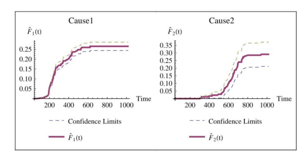
Figure 1 – Plot of estimate ofFj(t); j= 1,2 for mice mortality data

a definite analysis of the data. The first data give the survival times of mice, kept in a conventional germ-free environment, all of which were exposed to a fixed dose of radiation at an age of 5 to 6 weeks (Hoel (1972)). There are 3 causes of death viz thymic lymphoma (cause 1), reticulam cell sacroma (cause 2), and other causes (cause 3). This data were analysed by different researchers in various contexts (See Lawless (2003)). We treat other failures due to cause 3 as left censored observations. The estimates ofHj(t) and Fj(t)j = 1,2, are computed

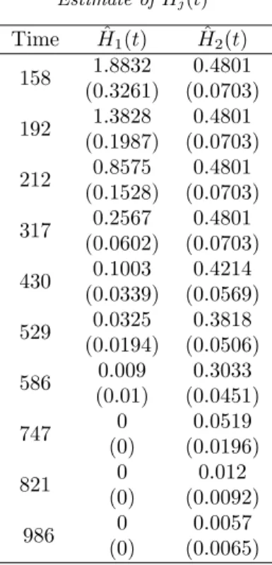
at diﬀerent time points. Forj= 1,2 the estimates ofHj(t) and its standard error

(written in parenthesis) are given in Table 5. Plots of ˆFj(t), j = 1,2 along with

95% conﬁdence limits are given in Figure 1. From Figure 1 it can be seen that ˆ

F1(t) predominates over ˆF2(t), which means that most of the initial failures are due to cause 1.

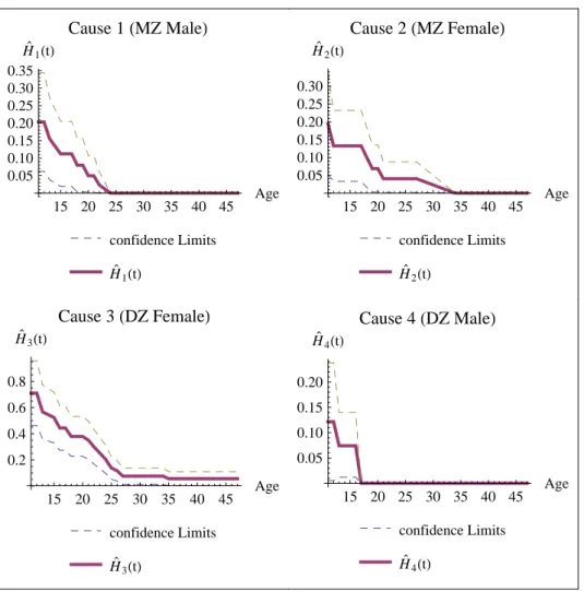
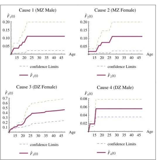
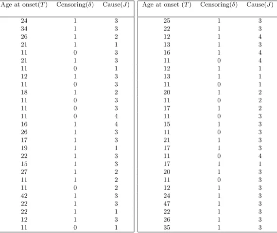
Now we consider the Australian twin data given in Duffyet al.(1990) which consists of information on the age at which appendectomy of monozygotic (MZ) and dizygotic (DZ) twins. The data are given in Table 6. Individuals having age less than 11 are considered as left censored observations. The data were analyzed in various contexts by different researchers (See Kalbfleisch and Prentice (2002), and Sankaran and Gleeja (2011)). We consider only the information on age of twin one from each pair. The types MZ male, MZ female, DZ male and DZ female pairs are considered as four different causes. Now the data are in the form of left censored lifetime data with multiple causes. It is therefore, more appropriate to model the data using cause specific reversed hazard rates, by including left censored observations.

The estimates ofHj(t) andFj(t), j= 1, ...4 are computed. The plots of

(15)

TABLE 5 Estimate of Hj(t)

Time Hˆ1(t) Hˆ2(t) 158 1.8832 0.4801

(0.3261) (0.0703) 192 1.3828 0.4801

(0.1987) (0.0703) 212 0.8575 0.4801

(0.1528) (0.0703) 317 0.2567 0.4801

(0.0602) (0.0703) 430 0.1003 0.4214

(0.0339) (0.0569) 529 0.0325 0.3818

(0.0194) (0.0506) 586 0.009 0.3033

(0.01) (0.0451)

747 0 0.0519

(0) (0.0196)

821 0 0.012

(0) (0.0092)

34 1 3

26 1 2

21 1 1

11 0 3

21 1 3

11 0 1

12 1 3

11 0 3

18 1 2

11 0 3

11 0 4

16 1 4

26 1 3

17 1 3

19 1 1

22 1 3

15 1 3

27 1 2

11 1 2

11 0 2

42 1 3

22 1 3

22 1 1

12 1 3

11 0 1

Age at onset (T) Censoring(δ) Cause(J)

25 1 3

22 1 3

12 1 4

13 1 3

16 1 4

11 0 4

12 1 1

13 1 1

11 0 1

20 1 2

11 0 2

17 1 2

11 0 3

15 1 3

11 0 3

21 1 3

17 1 3

11 0 4

17 1 1

20 1 3

11 0 3

12 1 3

24 1 3

47 1 3

22 1 3

26 1 3

(19)

7. Conclusion

In the present paper, we have introduced a new procedure using cause specific reversed hazard rates for modeling and analysis of left censored lifetime data with multiple causes. We proposed a non parametric estimator for the cumulative cause specific reversed hazard rates. The asymptotic properties of the estimators has been established using counting process method. Simulation studies establishes that the proposed procedure is efficient. The proposed method was applied to two real life data sets. Nonparametric tests for equality of cause specific hazard rates will be useful for comparing several risks. The work in this direction will be reported elsewhere.

ACKNOWLEDGEMENTS

We thank the editor and referee for their valuable comments and suggestions. The second author would like to thank Department of Science and Technology, Government of India for providing ﬁnancial support for this work under INSPIRE fellowship.

REFERENCES

P. K. Andersen, Ø. Borgan, R. D. Gill, N. Keiding (1993). Statistical Models Based on Counting Processes. Springer Verlag, New York.

R. E. Barlow, A. W. Marshall, F. Proschan (1963). Properties of prob-ability distributions with monotone hazard rate. The Annals of Mathematical Statistics, 34, no. 2, pp. 375–389.

H. W. Block,T. H. Savits,H. Singh(1998).The reversed hazard rate function. Probability in the Engineering and Informational Sciences, 12, pp. 69–90.

M. J. Crowder(2001). Classical Competing Risks. CRC Press, London. I. Dewan,S. Kulathinal(2007).On testing dependence between time to failure

and cause of failure when causes of failure are missing. PloS one, 2, no. 12, p. e1255.

D. L. Duffy, N. G. Martin, J. D. Mathews (1990). Appendectomy in

Aus-tralian twins. American Journal of Human Genetics, 47, no. 3, p. 590.

M. S. Finkelstein(2002). On the reversed hazard rate. Reliability Engineering & System Safety, 78, no. 1, pp. 71–75.

T. R. Fleming, D. P. Harrington (1991). Counting Processes and Survival

Analysis. John Wiley & Sons, New York.

R. C. Gupta, P. L. Gupta, R. D. Gupta(1998). Modeling failure time data

(20)

334 P. G. Sankaran and Anjana S R. C. Gupta,R. D. Gupta(2007).Proportional reversed hazard rate model and

its applications. Journal of Statistical Planning and Inference, 137, no. 11, pp. 3525–3536.

¨

U. G¨urler(1996).Bivariate estimation with right-truncated data. Journal of the American Statistical Association, 91, pp. 1152–1165.

D. G. Hoel(1972). A representation of mortality data by competing risks. Bio-metrics, 28, pp. 475–488.

J. H. Jeong,J. P. Fine(2009).A note on cause-specific residual life. Biometrika, 96, no. 1, pp. 237–242.

J. D. Kalbfleisch,R. L. Prentice(2002). The Statistical Analysis of Failure

Time Data, John Wiley & Sons, New York.

J. Keilson,U. Sumita(1982). Uniform stochastic ordering and related

inequal-ities. Canadian Journal of Statistics, 10, no. 3, pp. 181–198.

J. F. Lawless (2003). Statistical Models and Methods for Lifetime Data. John Wiley & Sons, New York.

A. W. Marshall,I. Olkin(2007). Life Distributions. Springer, New York. N. U. Nair, P. G. Sankaran, G. Asha (2005). Characterizations based on

reliability concepts. Journal of Applied Statistical Science, 14, no. 34, pp. 237– 242.

L. Peng, J. P. Fine (2007). Nonparametric quantile inference with competing– risks data. Biometrika, 94, no. 3, pp. 735–744.

D. Sengupta,A. K. Nanda(2010).The proportional reversed hazards regression

model. Journal of Applied Statistical Science, 18, no. 4, pp. 461–476.

SUMMARY

Modeling lifetime data with multiple causes using cause specific reversed hazard rates

In this paper we introduce and study cause specific reversed hazard rates in the context of left censored lifetime data with multiple causes. Nonparametric inference procedure for left censored lifetime data with multiple causes using cause specific reversed hazard rate is discussed. Asymptotic properties of the estimators are studied. Simulation studies are conducted to assess the efficiency of the estimators. Further, the proposed method is ap-plied to mice mortality data (Hoel (1972)) and Australian twin data (Duffyet al.(1990)).