Determination of Suitable Feedstock for Refineries Utilizing LP and NLP Models - Volume 1 Number 3 (Oct. 2010) - IJCEA

(1)

225

Abstract—One of the most vital steps in optimization and management of oil refineries is allocation of suitable feedstock. This becomes more crucial with fluctuation of crude oil price and down grading of its quality. The selected crudes should have suitable properties to meet the constraints of refinery units.The main crude properties which should be considered are boiling point curve, fractional specific gravity, fractional sulfur, bulk viscosity, RVP, Pour Point, metal content, bulk sulfur and bulk nitrogen content. In order to determine the optimum feedstock, a computer model was developed which contains different sections for crude oil characterization, optimum blending of petroleum cuts and modeling of refinery units. Several experiments were carried out on individual and blended crudes and the physical properties were measured and compared with the calculated results to validate the model. To determine the sulfur fraction in different cuts, the previously derived equations were tuned to cover wide range of crudes. The developed linear and nonlinear equations were utilized to determine the effects of variation of oil properties on distillation unit. Several test runs were collected from different refineries to validate the model.

Index Terms—Feedstock, LP, NLP, Refinery, Optimization

Nomenclature

AP: Aniline point (°C)

CABP: Cubic average boiling point (°C) CCR: Conradson carbon residue (wt%) CP: Cloud point (°C)

FPT: Flash point (°C) FRP: Freezing point (°C) Ind: Linearization index K: Watson K Factor l(x): Basic Lagrange function L(x): Lagrange function

MABP: Molar average boiling point (°C) MeABP: Mean average boiling point (°C) Mw: Molecular weight

Pb: Blend property Pi: Property of component i RMSE: Root mean squrw deviation RVP: Reid vapour pressure (psi) SP: Smoke point (°C)

S: Specific gravity TPP: Pour point(°C)

xi: Mass or Volume fraction of component i

Greek Symbols

α: Shape factor in distribution function β: Scale factor in distribution function ν: Viscosity (CSt)

∗ Modeling and Control Department, Research Institute of Petroleum Industry, Tehran 14665-137, IRAN(email:[email protected] ).

Γ: gamma distribution function

I. INTRODUCTION

Oil refining is one of the most complex chemical industries, which involves many different and complicated processes with various possible connections. Linear programming (LP) models have historically been used for scheduling and planning problems because of their ease of modeling and since they are relatively easy to solve. Refinery planning problems have been studied since the introduction of linear programming in 1950s [1]. Symonds [2] and Manne [3] applied linear programming techniques for long-term supply and production plans for crude oil processing and product pooling problems. The production planning optimization for refinery has been addressed by using linear and non linear programming in the past decades [4-8]. The main aim of production planning is to decide what to produce, how much to produce and when to produce for a given plan horizon in a company [9]. The objective of production planning in a refinery is to generate as many valuable products as possible, such as gasoline, jet fuel, diesel, and so on, and at the same time satisfying market demand and other constraints.

To formulate the refinery LP model, one can decompose the overall refinery problem in three subsystems[10]: (a) the crude-oil unloading and blending, (b) the production unit operations, and (c) the product blending and lifting (see Fig. 1). As it can be seen, one of the most important tasks in refinery planning is blending of crude oils and refinery products. Refinery feed is produced by blending different crude oil types with an specified blending ratio. On the other hand, The refinery products are manufactured by blending two or more different intermediate and final cuts. Some researches focus on product blending especially gasoline in which their objective function is the sale revenues[11-12]. Although the revenue is so important in blending calculations of refinery products, the most important subject is the properties of refinery feed and products. Each refinery has been designed to handel an specific crude oil with a limited range of properties( API, Sulfur fraction, viscosity, ...). If the refinery feed properties vary it affects different processing units and also it affects the refinery products specifications. Therfore different crude oils with different properties should be blended properly to prepare the refinery feedstock. In this research a suitable model has beed developed which characterises the crude oils, calculates the blended crude propertise and the optimum blending ratio of crude oils to produce a suitable feedstock.

Determination of Suitable Feedstock for

Refineries Utilizing LP and NLP Models

(2)

226 II. ALGORITHM

Developed algorithm contains three sections as follow: A.Crude oil characterization

B.Calculation of blended cut properties C.Calculation of optimum blending ratio

A. Crude oil characterization

Crude oil characterization is one of the most important tasks in refinery units modelling. This becomes more important when the cut has species with more than 10 carbon atoms. In this case, because of more hydrocarbons which have similar properties, it is difficult to characterize them. To solve this problem some researchers have tried to improve the analyses and databanks [13-14].

Fig. 1. Illustration of a standard refinery system [10]

The first and most important property which should be calculated is the full range boiling point curve of petroleum cut. Usually the boiling point of crude oils and petroleum cuts are stated based on percent distilled. Some of these boiling points are known experimentally and the full range should be calculated using interpolation and extrapolation methods. Two common algorithms of interpolation and extrapolation are Lagrange and probability distribution functions. The following polynomial should be used when utilizing Lagrange method:

∑

=

k

j j j

l

x

y

x

L

0

)

(

)

(

(1)

In which lj(x) is the basic Lagrange polynomial:

∏

≠

=

−

=

k

j i

i j i

i j

x

l

0

)

(

(2) In some cases especially for calculation of initial and final

boiling points, the probability distribution function could be used:

)

(

)

(

1

α

β

α

β α

Γ

=

−

x

e

x

p

(3) In which x is the variable, α and β are the shape and scale

factors respectively, and

Γ

(

α

)

is the gamma distribution function:

∫

∞

− −

=

Γ

0

1

)

(

_α

e

u

α

du

(4) Using probability distribution method, only two

parameters α and β should be known and the precision of calculation is evaluated using RMSE and R2_{as follow:}

n n

i yact ypred RMSE

∑

= −

= 1

2 ) (

(5)

2 ) 1(

1

2 ) (

1 2

∑

= −

∑

= −

−

= _n

i yact yact n

i yact ypred

R (6)

To develop a suitable algorithm for oil characterization, the measurable properties like density, boiling point curve and sulfur content have been used to calculate other properties. One of the most important parameters in crude oil characterization is the Watson k- factor which is defined as follows:

S MeABP K

3

= (7)

In this equation, S is the specific gravity and MeABP is the Mean Average Boiling Point and is calculated as:

∑ = = n

i xiTbi MABP

1 (8)

)

1 3

1 (∑

= = n

i xviTbi

CABP (9)

2 CABP MABP

MeABP= + (10)

In the mentioned equations, MABP and CABP are molar and cubic average boiling points respectively. xi and Tbi are cut i mass fraction and boiling point respectively.

Using equation (7) the Watson factor can be calculated. Watson factor can be used to calculate another properties such as molecular weight, Flash point, Aniline point,…which the corresponding equations are summarized in table 1.

TABLE1.EQUATIONS FOR CALCULATION OF CRUDE OIL PHYSICAL PROPERTIES[15]. No. Property Equation

11 Molecular weight ₅ ₂_.₁₉₆₂ ₁_.₀₁₆₄ 10

5673 .

4 × − −

= MeABP S

MW

12 Flash point

) 10 ( 10 log 001093 . 0 10 84947 . 2 014568 . 0

1

T T

FPT

+ +

(3)

227

13 Pour point

) 32834 . 0 310311 . 0 ( 100 ) 473575 . 0 61235 . 0 ( 970566 . 2 85 . 234 S S M S PP T − × − = ν

14 Aniline Point

S K MeABP AP 7 . 868 8 . 107 139 . 0 7 . 1253 + + − − =

15 Smoke point ln(SP)=−1.028+0.474K−0.00168MeABP

16 Freezing point

MeABP K S FRP 135 . 0 49 . 122 1826 42 . 2390 − + + − =

17 Cloud point

S MeABP MeABP P C 133 . 0 315 . 0 712 . 0 ) log( 49 . 5 41 . 7 log − − + − =

B. Calculation of blended cut properties

After crude oil characterization, the suitable blending equations should be used to calculate the blended crude properties. Using physical properties of individual crudes and suitable mixing rule, the blended property can be calculated. Some blended crude properties such as specific gravity, Sulphur content, asphaltene content, wax content, metal content, nitrogen content and acidity can be calculated linearly:

∑

=

n

i i i

b

x

P

1 ₍₁₈₎

In which Pb is the blend property, xi is component i mass or volume fraction and Pi is property of component i.

On the other hands, some properties such as viscosity, Pour point, smoke point, freezing point and flash point are mixed nonlinearly and we should use linearization index to calculate them:

)

(

)

(

1

∑

=

×

=

n i i i

b

x

Ind

P

Ind

(19) In which Ind is the index of properties and some of them

have been summarized in table 2.

TABLE2.PROPERTY INDICES FOR LINEARIZATION [16] Property Index Reid vapor pressure (RVP) P1.25 Viscosity Ln(ln(P+0.8)) Smoke point P 1 Freezing point )) 600 460 ln( 33 . 13

exp( P+

Pour point )) 600 460 ln( 5 . 12

exp( P+

Flash point )) 600 460 ln( 67 . 16

exp(− P+

C. Calculation of optimum blending ratio

The optimum blending ratio has been calculated by minimization of the following objective function:

2 1 mod

₎

(

∑

=

−

=

n i imix imix el i

P

f

(20) In which Pimodel and Pimix are the property i calculated by model and experimental data respectively. The optimization should be done subject to that the sum of blending ratios be equal to unity. The SQP method has been used for optimization.

III. RESULTS AND DISCUSSION

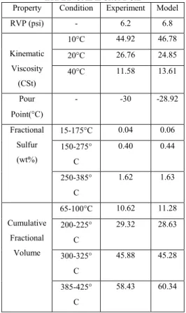
To validate the model, important properties of light and heavy crude oils have been calculate and compared with experimental data. Table 3 shows some calculated properties of Iranian OMIDIE crude oil and compares them with that of experimental data. Some crude oils were blended experimentally and their properties were measured and compared with the model results. Figure 2 represents the experimental and calculated boiling point curves of a crude oil which is a blend of 83 vol% Asmari and 17 vol% Darkhoein crudes. Some other experimental and calculated properties of this blended crude have been summarized in table 4. To validate the model in the blending ratio calculation, some crude have been blended experimentally and the blended crude properties have been fed into the model. The optimum blending ratio has been calculated using optimization algorithm as discussed in the previous section. Table 5 compares the calculated blending ratio of three crude oils with the experimental one. As seen, the model can acceptably represent the experimental data.

As a case study, the model has been used to substitute a portion of the present feed of an Iranian refinery with a blend of heavy crude oil and condensate. The present feed of this refinery is OMIDIE crude. Table 6 shows the blending ratios of substitute feed which have been calculated using the developed model. The boiling point curves and product distribution of present and substitute feeds are represented in figures 3 and 4 respectively. Also the main properties of two feeds are shown in table 7.

(4)

228

Figure 2. Comparison of calculated and experimental TBP curve of a blended crude oil (83 vol% Asmari and 17 vol% Darkhoin crudes) TABLE3.SOME CALCULATED AND EXPERIMENTAL PROPERTIES OF

IRANIAN OMIDIE CRUDE OIL

Model Experiment Condition

Property

6.8 6.2

RVP (psi)

46.78 44.92

10°C Kinematic

Viscosity (CSt)

24.85 26.76

20°C

13.61 11.58

40°C

-28.92 -30

Pour

Point(°C)

0.06 0.04

15-175°C Fractional

Sulfur (wt%)

0.44 0.40

150-275°

C

1.63 1.62

250-385°

C

11.28 10.62

65-100°C

Cumulative Fractional

Volume

28.63 29.32

200-225°

C

45.28 45.88

300-325°

C

60.34 58.43

385-425°

C

TABLE 4.SOME CALCULATED AND EXPERIMENTAL PROPERTIES OF A

BLENDED CRUDE OIL (83 VOL%ASMARI AND 17 VOL%DARKHOIN CRUDES) Model

Experiment Property

0.8625 0.8625

Specific Gravity

1.54 1.65

Sulfur (wt %)

-14 -17

Pour Point (°C)

20.7 18.8

Kinematic viscosity @10°C (cst)

6.69 6.72

Kinematic viscosity @40°C (cst)

5.66 5.69

Wax (wt %)

TABLE5.CALCULATION OF OPTIMUM BLENDING RATIO

Crude Experimental mixing ratio

Calculated mixing

ratio

A 30 30

B 53 50

C 17 20

TABLE6. THE BLENDING PERCENT OF SUBSTITUTE FEED OF AN IRANIAN

REFINERY

Substitute Cuts Blending Volume

Percent

Heavy Oil (API=19.7) 32.4 Condensate (API=59) 10

OMIDIE Crude (API=28.06)

57.6

Fig. 3. The boiling point curves of the present and substitute feeds of selected refinery

Fig. 4. Product distribution of the present and substitute feeds of selected refinery

TABLE7.THE MAIN PROPERTIES OF THE PRESENT AND SUBSTITUTE FEEDS OF SELECTED REFINERY

Property Present Feed Substitute Feed

API 28.06 28.06 Sulfur (wt%) 2.37 2.56 Asphaltene (wt%) 4.34 5.87 Wax (wt%) 5.17 4.83 Metals(ppm) 117.7 115.9 Acidity(mgKOH/gr) 0.105 0.104

RVP(psi) 6.2 6.0

CCR (wt%) 6.85 7.81

IV. CONCLUSION

(5)

229 Sufficient experimental data of light and heavy crudes have been used to validate the model. The results revealed that different types of crudes with different API in the range of 15 to 50 could be fed to refineries with suitable blending.

REFERENCES

[1] P. C. P. Reddy, I. A. Karimi, R. Srinivasan,A new continuous time formulation for scheduling crude oil operations, Chemical Engineering Science, 59 (2004) 1325- 1341

[2] G. H. Symonds, Linear programming: The solution of refinery problems, ESSO Standard Oil Company (1955) New York

[3] A. S. Manne, Scheduling of petroleum operations, Harvard University Press, Cambridge (1956)

[4] N. Shah, ' Mathematical programming techniques for crude oil scheduling, Computers and Chemical Engineering, 20(1996) 1227-1232

[5] W. Li, C. W. Hui, B. Hua, T. Zhongxuan, Scheduling crude oil unloading, storage and processing, Industrial and Engineering Chemistry Research, 41(2002) 6723-6734

[6] P. C. P. Reddy, I. A. Karimi, R. Srinivasan, A novel solution approach for optimizing crude oil operations, AIChE Journal, 50,6(2004) 1177-1197

[7] K. C. Furman. Z. Jia, M. G. Ierapetritou, A robust event-based continuous time formulation for tank transfer scheduling, Industrial and Engineering chemistry Research, 46 (26), (2007) 9126-9136 [8] R. Karuppiah, K. C. Furman, I. E. Grossmann, Global optimization for

scheduling refinery crude oil operation, Computers & Chemical Engineering 32 (11) (2008), pp. 2745–2766

[9] GAO Zhen , TANG Lixin , JIN Hui , XU Nannan , An Optimization Model for the Production Planning of Overall Refinery, Chinese Journal of Chemical Engineering, 16( I) (2008) 67-70

[10] C. A. Mendez, I. E. Grossmann, I. Harjunkoski, P. Kabore, A simultaneous optimization approach for off- line blending and scheduling of oil- refinery operation, Computers and chemical Engineering, 30 (2006) 614-634

[11] Julija Ristic, Loreta Tripceva- Trajkovska, Ice Rikaloskit, Liljana Markovska, OPTIMIZA TION OF REFINERY PRODUCTS BLENDING, Bulletin of the Chemists and Technologists of Macedonia, Vol. 18, No. 2, pp. 171-178 (1999)

[12] Dinesh K. Khosla , Santosh K. Gupta, Deoki N. Saraf," Multi-objective optimization of fuel oil blending using the jumping gene adaptation of genetic algorithm", Fuel Processing Technology 88 (2007) 51–63 [13] M.Dente, E.Ranzi, G.Bozzano, T.Faravelli, P.J.M.Valkenburg; Heavy

Component Description in the kinetic modelling of Hydro conversion pyrolysis ; AIChE Spring National Meeting; April 23; (2001) [14] J.E.Gwyn; Universal yields models for the steam pyrolysis of

hydrocarbon to olefin; Fuel Process Technology;170; (2002)1-7 [15] PHYSICAL PROPERTIES, Chemstations Inc. 2901 Wilcrest Drive,

Suite 305 Houston, Texas 77042, U.S.A.