NUMERICAL APPROXIMATION OF SPECTRUM FOR VARIABLE COEFFICIENTS EULER-BERNOULLI BEAMS UNDER A FORCE CONTROL IN POSITION AND VELOCITY

(1)

ISSN: 1311-1728 (printed version); ISSN: 1314-8060 (on-line version) doi:_{http://dx.doi.org/10.12732/ijam.v30i3.1}

Kouassi Ayo Ay´ebi´e Hermith1§_{, Coulibaly Adama}2_,

Tour´e Kidj´egbo Augustin3

1_{Université Félix Houphouët Boigny}

Yamoussoukro, BP 2444, C ˆOTE D’IVOIRE

2_{Université Félix Houphouët Boigny}

BP 582, Abidjan 22, C ˆOTE D’IVOIRE

3_{Institut National Polytechnique Houphou¨et-Boigny}

Yamoussoukro, BP 2444, C ˆOTE D’IVOIRE

Abstract: In this paper, we use asymptotic techniques and the finite differ-ences method to study the spectrum of differential operator arising in exponen-tial stabilization of Euler-Bernoulli beam with nonuniform thickness or density that is clamped at one end and is free at the other. To stabilize the system, we apply at the free end, the following shear force feedback control:

(EI(_·)uxx(·, t))x(1) =αu(1, t) +βut(1, t), t >0.

We build a numerical scheme and investigate the eigenvalues locus as a function of the positive feedback parameters α and β.

AMS Subject Classification: 93C20, 93D15, 35B35, 35P10

Key Words: numerical approximation problem, semigroup theory, asymp-totic behavior, exponential stability, finite differences

Received: March 9, 2017 c 2017 Academic Publications

(2)

1. Introduction

Consider the following evolutive system:

(S1) :      

    

utt(x, t)−uxx(x, t) = 0, 0< x <1, t >0,

u(0, t) = 0,

ux(1, t) =₋βut(1, t), t >0,

(1)

whereuis a scalar function of variablesxandt,βis a nonzero positive constant. This simplified model represents for example a cable clamped at one end and is submitted to a linear boundary control force in velocity at the free end. The cable is supposed flexible with constant length.

Many authors have studied the above system (see [5] for example and the references therein) and have proved that the system (S1) is exponentially stable

for allβ ₆= 1. Moreover, they have proved that the system (S₁) verifies the Riesz basis property and obtained the spectrum by an explicit formula.

The idea of adding a control force in position to the existing feedback has been invoked by the studies of many authors (see [4]).

Consider the following system:

(S2) :      

    

utt(x, t)₋uxx(x, t) = 0, 0< x <1, t >0,

u(0, t) = 0, t >0,

ux(1, t) =₋αu(1, t)₋βut(1, t), t >0.

(2)

From mathematical point of view one wants to check if the properties of the disrupted system stay intact. To this question many authors have provided a positive answer. The system (S₁) obtained by disruption of system (S₁) is exponentially stable again (see [10]) and verifies the Riesz basis property (see [14]).

From practical point of view, the goal is to improve the optimal decay rate of energy. To this practical preoccupation which takes its importance from cost of the realization of models thus obtained theoretically, it should provide a satisfactory answer. The theoretical study of such problem, is not easy even for a simple model like the system (S1).

(3)

property and the exponential stability has negative effect on the optimal decay rate of elastic energy.

In [8] the authors use the finite differences method and the QZ method to describe geometrically the spectrum and have got the same results.

So the idea of using numerical methods to study the impact of adding a control to an existing control, seems to be a credible alternative.

In this paper we consider the evolutive system given by:

         

        

m(x)utt(x, t) + (EI(x)uxx(x, t))xx = 0, 0< x <1, t >0,

u(0, t) =ux(0, t) =uxx(1, t) = 0, t >0,

(EI(_·)uxx(·, t))_x(1) =αu(1, t) +βut(1, t), t >0,

u(x,0) =u0(x) ;ut(x,0) =u1(x), 0< x <1,

(3)

where α, β are two given positive constants, u(x, t) stands for a transversal deviation of the beam at position x and time t, a subscript letter denotes the partial derivation with respect that variable. The length of the beam is chosen to be unity, EI(.) is the stiffness of the beam, and m(.) is the mass density. Moreover, we shall always assume that:

m(_·), EI(.)_∈C4(0,1) and m(x), EI(x)>0. (4) For α = 0, many authors have proved the Riesz basis property and the expo-nential stability (see [2], [12]).

In this paper one uses the finite differences method and the QZ method to answer the following question: does the control in position improve the optimal decay rate of elastic energy? The main goal of this work is to use the finite differences method to elaborate a program that gives the complete eigenvalues location of the system defined by (3), as a function of positive feedback parameters α andβ.

(4)

2. Formulation of the System (3) in the Context of the C₀₋Semigroup of Contractions Theory

Let us introduce the following spaces:

V_E2=

u(x)_∈H2(0,1) :u(0) =ux(0) = 0 , (5)

H₌_V_E2₍₀_,₁₎_×_L2₍₀_,₁₎_, ₍₆₎ D(0,1) = the space of smooth functions with compact support,

D′(0,1) = the space of continuous linear functions,

f :D(0,1)_→C_.

The superscript T stands for the transpose and the spaces L2(0,1) and

Hk₍₀_,_{1) are defined as}

L2(0,1) =

u: [0,1]_→R_: Z 1

0

u2dx <_∞

(7)

Hk(0,1) =nu: [0,1]_→R_:_{u, u}(1)_{, . . . , u}(k)_∈_L2₍₀_,₁₎o_. ₍₈₎

In the spaceH_{, we define the inner-product}

hu, v_iH =

Z 1 0

m(x)f₂(x)g₂(x) +EI(x)f₁′′(x)g′′ 1(x)

dx

+αf1(1)g1(1), (9)

whereu= (f1, f2)T ∈Hetu= (g1, g2)T ∈H.

Next, we define an unbounded linear operatorA_:D(A₎_⊂H_→H_{as follows:}

A₍_{f, g}_{) =}

g(x),₋ 1

m(x) EI(x)f

′′₍_x₎′′

, (10)

whereD(A₎_,_{the domain of operator, is}

D(A_{) =}n₍_{f, g}₎T _∈_H4₍₀_,₁₎_∩_V2

E(0,1)×VE2(0,1) :

f′′(1) = 0, EI(_·)f′′(_·)′′(1) =αf(1) +βg(1)o. (11)

With these notations, the set of system (3) can be formally written as

  

 

dY (t)

dt =AY (t),

Y (0) =Y0∈H,

(12)

(5)

Theorem 1. The operator A_{, defined by} ₍₁₀₎ _and _{(11), generates a}

C₀₋semigroup of contractions onH_.

Proof. See [13].

3. Spectrum of Operator A

Now we are ready to study the eigenvalue problem of A_.

Letλ_∈σ(A_{) and Φ = (}φ,Ψ) be an eigenfunction ofA_{corresponding to} λ. Then we have Ψ =λφ and φsatisfies the following equation:

       

      

λ2m(x)φ(x) + (EI(x)φ′′₍_x₎₎′′

= 0, 0< x <1,

φ(0) =φ′(0) =φ′′(1) = 0,

φ′′′(1) = 1

EI(1)(α+βλ)φ(1).

(13)

Expanding (13) yields for all 0< x <1,

         

        

φ(4)(x) +2EI

′₍_x₎ EI(x) φ

′′′₍_x_{) +}EI′′(x) EI(x) φ

′′₍_x_{) +}λ2m(x)

EI(x) φ(x) = 0,

φ(0) =φ′_{(0) =}_φ′′_{(1) = 0}_,

φ′′′_{(1) =} 1

EI(1)(α+βλ)φ(1).

(14)

In order to simplify our computations, we introduce a spatial scale transforma-tion in x:

f(z) =φ(x), z(x) = 1

p Z x

0

m(ζ)

EI(ζ)

1₄ dζ,

where

p=

Z 1 0

m(ζ)

EI(ζ)

14

(6)

Then, (14) together with its boundary conditions can be transformed into                           

f(4)(z) +a(z)f′′′₍_z_{) +}_b₍_z₎_f′′₍_z_{) +}_c₍_z₎_f′₍_z_{) +}_λ2_p4_f₍_z_{) = 0}_,

0< z <1,

f(0) =f′_{(0) = 0}_,

z_x2(1)f′′(1) +zxx(1)f′(1) = 0,

f′′′(1) + 3zxx(1)

z2

x(1)

f′′(1) + zxxx(1)

z3

x(1)

f′(1)₋ (α+λβ)

z3

x(1)EI(1)

f(1) = 0,

(16)

with

a(z) = 6zxx

z2

x

+ 2EI

′₍_x₎ zxEI(x)

(17)

b(z) = 3z

2

xx

z4

x

+6zxxEI

′₍_x₎ z3

xEI(x)

+ EI

′′₍_x₎ z2

xEI(x)

+ 4zxxx

z3

x

(18)

c(z) = zxxxx

z4

x

+2zxxxEI

′₍_x₎ z4

xEI(x)

+zxxEI

′′₍_x₎ z4

xEI(x)

(19)

zx = 1

p

m(x)

EI(x)

1 4

, z_x4 = 1

p4 m(x)

EI(x) (20)

and

zxx = 1 4p

_m

(x)

EI(x)

−

3

4 d

dx _m

(x)

EI(x)

1 4

. (21)

The equation in (16) is

f(4)(z) +a(z)f′′′(z) +b(z)f′′(z) +c(z)f′(z) +λ2h4f(z) = 0,

0< z <1.

This can be further implied by applying another invertible transformation:

g(z) = exp

1 4

Z z

0

a(ζ)dζ

f(z), 0< z <1, (22)

(7)

original one for all 0< z <1:                   

g(4)(z) +a1(z)g′′(z) +a2(z)g′(z) +a3g(z) +λ2p4g(z) = 0, g(0) =g′(0) = 0,

g′′(1) +a11g′(1) +a12g(1) = 0, g′′′_{(1) +}_a

21g′′(1) +a22g′(1) +a23g(1) = 0,

(23)

where

a1(z) = −

3 2a

′₍_z₎ −3

8a

2₍_z_{) +}_b₍_z₎_, a2(z) =

1 8a

3₍_z₎₋1

2a(z)b(z)−a

′′₍_z_{) +}_c₍_z₎_,

a3(z) =

3 16a

′2₍_z₎

− 1₄a′′′(z) + 3 32a

′₍_z₎_a2₍_z₎

−₂₅₆3 a4(z) +b(z)

1 16a

2₍_z₎

− 1₄a′(z)

−a(z)₄c(z),

a11 = −1

2a(1) +

zxx(1)

z2

x(1)

,

a12 =

1 16z

2

x(1)a2(1)− 1 4z

2

x(1)a′(1)− 1

4zxx(1)a(1)

z2

x(1)

,

a21 = −

3 4a(1) +

3zxx(1)

z2

x(1)

,

a22 = −

3 4a

′_{(1) +} 3

16a

2₍₁₎₋3zxx(1)a(1)

2z2

x(1)

+zxxx(1)

z3

x(1)

,

a23 = −

1 4a

′′_{(1) +} 3

16a

′₍₁₎_a₍₁₎

−₆₄1 a3(1)₋3zxx(1)a

′₍₁₎

4z2

x(1) +3zxx(1)a

2₍₁₎

16z2

x(1) −

3zxxx(1)a(1) 4z3

x(1) −

(α+λβ)

z3

x(1)EI(1)

,

a₂₃ = θ₀₋ λβ z3

x(1)EI(1)

, with

θ₀ = ₋1 4a

′′_{(1) +} 3

16a

′₍₁₎_a₍₁₎

−₆₄1 a3(1)₋3zxx(1)a

′₍₁₎

4z2

x(1) +3zxx(1)a

2₍₁₎

16z2_x(1) −

3zxxx(1)a(1) 4z3_x(1) −

(8)

Theorem 2. Let A _{be defined by} ₍₁₀₎ _and _{(11), then an asymptotic}

expression of the eigenvalues of the problem (23)is given by

λn =

. √

2

2p2 (µ3−µ2)±

1

p2 "

. √

2

2 (µ3+µ2) +

n+1

2

2 π2

# i

+O

1

n

, (24)

wheren=N, N + 1, . . . withN large enough, and

µ3−µ2 = 2 √

2 β

z3

x(1)EI(1)p2 =₋2

√

2βp EI(1)

m(1)

EI(1)

−

3 4

, (25)

µ3+µ2 = 2 √

2 (µ1+b11). (26)

Moreover,λn(n=N, N + 1, . . .)with sufficiently large modulus are simple and distinct except for finitely many of them, and satisfy

lim

n→+∞Re(λn) =−

2β pEI(1)

m(1)

EI(1)

−

3 4

.

Proof. (See [13]).

4. Finite Differences Method

In this section, we use the finite differences method to study numerically the spectrum of operator of the problem (3), see P.G. Ciarlet [3], J. Rappaz and M. Picasso [11]. Then, we apply QZ method, see G.H. Golub [7], C.B. Moler and G.W. Stewart [9]. Finally, we study the influence of parameters α, β in velocity convergence of the system (3). The length of the beam is chosen to be unity, EI(x) = (1 +x)4, is the stiffness of the beam, and m(x) = (1 +x)2 is the mass density.

(9)

Hence we get the following system 0< x <1:

           

          

u(4)(x) +a1(x)u′′(x) +a2(x)u′(x) +a3(x)u(x)

+λ2p4u(x) = 0, u(0) =u′_{(0) = 0}_,

u′′(1) +a11u′(1) +a12u(1) = 0,

u′′′(1) +a21u′′(1) +a22u′(1) +a23u(1) = 0.

(27)

We develop a numerical scheme based on the finite differences method for the eigenvalue problem (27) associated with the evolutive system defined by (3). In practical, the spectral problem is not simple and cannot be solved by formula. Even when there is a formula, it might be so complicated that we would prefer to visualize the eigenvalues by looking at a graph. The finite differences method is one of the best known of the most important techniques of computation using quite simple equations and consists of replacing each derivative by a difference quotient. Consider for instance, a functionu :x_7→u(x) of variable

x. Choose a mesh size h = 1

n for all n∈N

∗_{. We approximate the value} _u₍_x

i) forxi =ih, i= 0,1, . . . , n and x0 = 0, xn= 1, by a number ui indexed by an integer i:ui ∼u(xi). Using Taylor expansions, we get for the derivatives, the following approximations for i= 2, . . . , n₋2:

u′(xi) = −

3u(xi) + 4u(xi+h)−u(xi+ 2h)

2h +O h

2

, (28)

u′′(xi) = u(xi−h)−2u(xi) +u(xi+h)

h2 +O h 2

, (29)

u(4)(xi) =

u(xi−2h)−4u(xi−h) + 6u(xi)

h4 +

−4u(xi+h) +u(xi+ 2h)

h4 +O h 2

. (30)

The approximations of the boundary conditions give:

u0= 0, 4u1−u2 = 0, (31)

whereu(xi) =ui, fori= 0,1, . . . , n.

Expanding the functionu:x_7→u(x) according to its Taylor series of order 4, we get:

u(1₋h) =u(1)₋hu′(1) + h

2

2!u

′′₍₁₎ −h

3

3!u

′′′_{(1) +} h4

4!u

(4)₍_ξ

(10)

u(1₋2h) =u(1)₋2hu′(1) + 2h2u′′(1)₋ 8h

3

3! u

′′′_{(1) +} 16h4

4! u

(4)₍_ξ

2), (33) u(1₋3h) =u(1)₋3hu′(1) +9h

2

2! u

′′₍₁₎ −27h

3

3! u

′′′_{(1) +} 81h4

4! u

(4)₍_ξ

3), (34)

withξj ∈]1−jh,1[, j= 1,2,3.

We eliminate u′′(1) (respectively u′(1)) in equations (32) and (33) we get:

u′(1) = u(1−2h)−4u(1−h) + 3u(1)

2h +O h

2

, (35)

u′′(1) = u(1−2h)−2u(1−h) +u(1)

h2 +O h 2

. (36)

We eliminate u′(1) in equations (32), (33) and (34) we get:

u′′′(1)_≃ −u(1−3h) + 3u(1−2h)−3u(1−h) +u(1)

3h3 . (37)

The approximation of the system (27) is:

                              

ui−2+aiui−1+ bi+λ2p4h4

ui+ciui+1+diui+2= 0, i= 2, . . . , n₋2,

u0 = 4u1−u2 = 0,

(2 +ha11)un−2−(4 + 4ha11)un−1+ 2 + 3ha11+ 2a12h2un= 0,

−2un−3+ 6 + 6a21h+ 3a22h2un−2+ −6−12a21h−12a22h2un−1

+

2 + 6a21h+ 9a22h2+ 3θ0h3−

3λβh3 z3

x(1)EI(1)

un= 0,

(38) where

ai = −4 +a1ih2, (39)

bi = 6−2h2a1i− 3 2a2ih

3₊_a

3ih4, (40)

ci = −4 +a1ih2+ 2a2ih3, di= 1−

a1i 2 h

3_, ₍₄₁₎

θ0 = a23+

λβh3 z3

x(1)EI(1)

, (42)

(11)

a1i =a1(xi), a2i =a2(xi) and a3i=a3(xi), i= 2, . . . , n−2.

The system (38) can be written following form:

                              

λ2u1−1₄λ2u2 = 0,

ui−2+aiui−1+ bi+λ2p4h4

ui+ciui+1+diui+2= 0, i= 2, . . . , n₋2,

(2 +ha11)un−2−(4 + 4ha11)un−1+ 2 + 3ha11+ 2a12h2un= 0,

−2un−3+ 6 + 6a21h+ 3a22h2

un−2+ −6−12a21h−12a22h2

un−1

+

2 + 6a₂₁h+ 9a₂₂h2+ 3θ₀h3₋ 3λβh 3 z3

x(1)EI(1)

un= 0.

(43) We can calculate u1, . . . , un using the scheme for the partial differential equation. Here the finite differences method looks for the complex number λ

such as there exists a nonzero vector

U = (u1, u2, ..., un)T satisfies the above discrete problem (43). Now, we consider the matricesA, B, C of order n, defined as follows:

Aij =

                  

1 for i=j= 1,

−14 for i= 1, j= 2,

p4h4 for i=j= 2, . . . , n₋2,

0 elsewhere,

Bij =

              

−βh3 3 z3

x(1)EI(1)

for i=j=n,

0 for i=j= 1, . . . , n₋1,

(12)

Cij =                           

bi if i=j,

ai if j=i−1,

ci if j=i+ 1,

di if j=i+ 2,

1 if j=i₋2.

                                                            

C₁₁ = 0, C12 = 0,

Cn−1n−2 = 2 +ha11, Cn−1n−1 = −4−4ha11

Cn−1n = 2 + 3ha11+ 2a12h2, Cnn−3 = −2,

Cnn−2 = 6 + 2ha21+a22h2, Cnn−1 = −6−12ha21−12a22h2,

Cnn = 2 + 6ha21+ 9a22h2+ 3θ0.

The problem (43) takes the following equation form:

λ2AU +λBU +CU = 0, (44) where the matrices A, B, andC are defined as above, and where

U = (u1, u2, ..., un)T . (45) Now, we introduce the auxiliary vector:

Z =λU, (46)

(13)

 



AZ = λAU

−CU = λAZ+λBU,

(47)

which is equivalent to the system:

A 0

0 ₋C

Z U

=λ

0 A

A B Z U

. (48)

We get a generalized eigenvalue problem:

MV =λNV (49)

with

M =

A 0

0 ₋C

, N =

0 A

A B

and V = (Z, U)T.

And we use QZ method to resolve this problem.

5. Numerical Experiments

To evaluate the effect of parametersα and β on the spectrum, we give here in the same field, the graphs of the spectrum for different values of the control in positionα and velocity β.

We do the study for three cases:

First case : α= 0 a) We take β_∈]0; 1[.

We observe that when the parameterβ _∈]0; 1[ without control in position

α, the location of spectrum moves rapidly on the left-hand side of the complex plane.

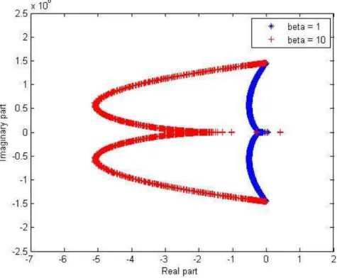
b) We takeβ _≥1.

We observe that when the parameterβincreases without control in position

α, the location of spectrum moves rapidly on the left-hand side of the complex plane.

Second case α >0:

a) β _∈]0; 1[.We fix α= 10 and takeβ = 0.1 andβ = 0.3.

We observe that when the parameter β _∈ ]0; 1[ for a fixed value ofα >0, the location of spectrum moves rapidly on the left-hand side of the complex plane.

(14)

Figure 1: Effect of parameter β _∈]0; 1[ on the spectrum for α= 0.

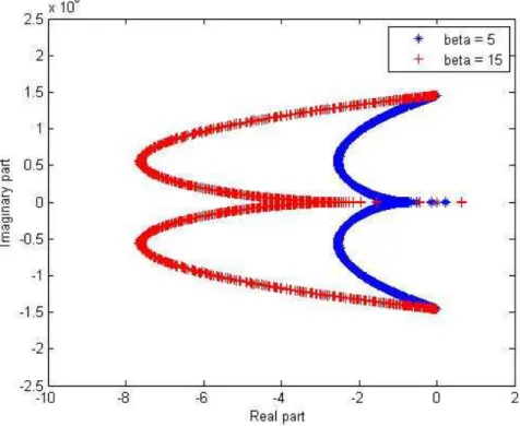
We observe that when the parameterβ increases for a fixed value ofα >0, the location of spectrum moves rapidly on the left-hand side of the complex plane.

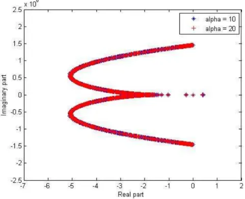
Third case:

We fixe β= 10 and take α= 10 andα = 20.

We observe that the parameter α has not effect on the spectrum for a fixed value of β and the location of spectrum stays on the left-hand side of the complex plane.

(15)

Figure 2: Effect of parameterβ _≥1 on the spectrum forα = 0.

permits to appreciate the impact of the control force in position on the optimal decay rate of the studied system energy.

References

[1] M.D. Aouragh and N. Yebari, Stabilisation exponentielle d’une équation des poutres d’Euler-Bernoulli à coefficients variables, Annales Mathématiques Blaise Pascal,16, No. 2 (2009), 483-510.

[2] B.Z. Guo, Riesz basis property and exponential stability of controlled Euler-Bernoulli beam equation whith variable coefficients, SIAM J. Con-trol Optim.,40, No. 6 (2002), 1905-1923.

(16)

Figure 3: Effect of parameterβ _∈]0; 1[ on the spectrum forα = 10.

[4] M. Cherkaoui, F. Conrad, N. Yebari, Optimal decay rate of energy for wave equation with boundary feedback,Advances in Mathematical Sciences and Applications, 12(2002), 549-568.

[5] S. Cox, E. Zuazua, The rate at which energy decays in a damping string,

Comm. Partial Differential Equations, 19(1994), 213-243.

[6] R.F. Curtain and H.J. Zwart, An Introduction to Infinite Dimensional Linear System Theory, Springer Verlag, New York (1995).

[7] G.H. Golub and C.F.V. Loan, Matrix Computations, The Johns Hopkins University Press (1989).

(17)

Figure 4: Effect of parameterβ _≥1 on the spectrum forα= 10.

[9] C.B. Moler and G.W. Stewart, An algorithm for generalized matrix eigen-value problems,SIAM J. Numer. Anal.10 (1973), 241-256 (Collection of articles dedicated to the memory of George E. Forsythe).

[10] ¨O. Morg¨ul, A dynamic control law for the wave equation, Automatic, 30, No. 11 (1994), 1785-1792.

[11] J. Rappaz and M. Picasso,Introduction `a l’analyse num´erique, Press Poly-techniques et Universitaires, Lausanne (1998).

[12] P. Rideau, Contrôle d’assemblage de poutres flexibles par des capteurs ac-tionneurs ponctuels: étude du spectre du système,Thèse, École Nationale Supérieure des Mines de Paris, Sophia-Antipolis (1985).

(18)

Figure 5: Effect of parameter α on the spectrum forβ fixed.

in position and vellocity. Far East Journal of Applied Mathematics, 88, No. 3 (2014), 193-220.