ISSN: 1311-1728 (printed version); ISSN: 1314-8060 (on-line version) doi:http://dx.doi.org/10.12732/ijam.v30i2.2
PRICING OPTION UNDER STOCHASTIC VOLATILITY DOUBLE JUMP MODEL (SVJJ)
Manal Bouskraoui1, Aziz Arbai2§
1Department of Mathematics and Statistics University Abdelmalek Essaadi at Tanger
St., 11 Elasmai borj II, Essaouira – 44 000, MOROCCO 2Navarre place, San Francisco 3
Tanger – 9000, MOROCCO
Abstract: Through this paper, we introduce Fourier transform as an alter-native approach to pricing option when the underlying asset follows Stochastic Volatility double Jump model (SVJJ). In fact the weakness of the traditional approaches does not depend on closed formula of probability density function which is explicitly unknown under this model. The advantage of Fourier trans-form technique is that for a wide class of stock price the only thing necessary to evaluate European call is a so called characteristic function since there is one-to-one relation-ship between a p.d.f & ch.f and both of which uniquely de-termine a probability distribution. For accuracy and validation we implement pricing formulas FFT, Monte Carlo simulation and we compare both of them to the benchmark model BS.
AMS Subject Classification: 60H15
Key Words: Fourier transform, risk-neutral option pricing, stochastic volatil-ity, jump-diffusion, Monte-Carlo simulation
1. Introduction
Although the fame of Black & Scholes formula [4], [12], this log-normal pure Received: January 8, 2017 c 2017 Academic Publications
diffusion model miscalculate option. First of all, model leaves out the effect of jump size uncertainty of return volatility and the arrival of abnormal informa-tion [13]. Moreover, normality distribuinforma-tion contradict empirical evidence. In fact, market exhibit a non-zero skewness and higher kurtosis.
Luckily, the stochastic volatility double jump model corrects this flaw [11]. The literature point out that this model [7], [15] and [1] is the most accurate one to describe precisely the logarithm underlying asset price distribution with stochastic volatility under jumps [14]. However, the problem arises when the probability density function is not explicitly known in term of closed formula.
In this paper, we will discuss the problem of valuing a European call option though Fourier transform (see [5], [15]). This approach is able to give in wide class of underlying asset a distribution of the model by substitutes as so called a characteristic function in some predefined integral. We present the outline of this paper in Section 2 where we briefly describe SVJJ model. Then, in Section 3 and Section 4 we present the characteristic function of the model and show the accurate closed form expression of Fourier inversion transform option pricing. Finally, we conclude with numerical results.
2. Stochastic Volatility Double Jump 2.1. Model Descriptions
Throughout this section, we consider a complete probability space (Ω,F, P) with an information filtration {Ft; 0≤t≤T}, satisfying the usual conditions. We denote by {e−rtSt; 0 ≤ t ≤ T} a discounted asset price process where T is a finite time horizon. In an arbitrage-free market, prices of any asset can be calculated as an expected terminal payoffs under discounted by a risk-free interest rate r such that EQ[e−rTS
T|Ft] = e−rtSt, which is a martingale condition. We define the stochastic volatility double Jump model (SVJJ) as
dSt= (r−λsκ)Stdt+
p
VtStdBts+Js(Y)St−dNts, (1) dVt=ǫ(¯v−Vt)dt+σ
p
VtdBtv+Jv(Z)dNtv. (2) Here r is the riskless interest rate which is assumed to be constant, ǫ ≥ 0, ¯v ≥ 0 and σ > 0 are called the speed of mean reversion, the mean level of variance and the volatility of the volatility, respectively. Furthermore, the Brownian motions Bs and Bv are assumed to be correlated with correlation coefficient ρ. Ns
intensitiesλsandλvrespectively. Moreover, we assume that the jump processes Nts and Ntv are independent with standard Brownian motion Bs and Bv.
In equation (1), Js(Y) (rep. Jv(Z)) is the Poisson jump-amplitude. Y (resp. Z) is an underlying Poisson amplitude mark process selected defined as Y = ln(1 +J(Y)).
For convenience, Nts (resp. Ntv) is the standard Poisson jump counting process with jump intensity λs(resp. λv) and expected valueλsdt(resp. λvdt). Also, the symbolic jump term for the asset price and volatility respectively are
Js(Y)dNts= dNs
t
X
i=1
Js(Yi),
Jv(Z)dNts = dNv
t
X
j=1
Jv(Zj).
HereYi(resp. Zj) is theith(resp. jth) jump-amplitude random variable taken from a set of independent, identically distributed random variables. We assume that the density of both jump-amplitude Y and Z are receptively log-normal and exponential distributed (see [15])
φY(y)∼ N(ln(1 +µ)− 1 2δ
2, δ2), (3)
φZ(z)∼exp(1
ζ). (4)
3. European Call Option Price
In this section, we want to price a European call option by using the PDE approach which is by now quite standard in literature (see e.g. Heston [10], Bates [3], Bakshi [1]). We let C denote the price at timet of a European style call option on St with strike price K and expiration time T = t+τ. Using the fact that a terminal payoffs of an European call option on the underlying assetStwith strike priceK is max(St−K,0) and assuming that the short-term interest rate r is constant over the lifetime of the option. European call price at timetis computed as discounted risk-neutral conditional expectations of the terminal payoffs
where EQ (resp. Q(.)) is the conditional expectation with respect to the risk-neutral probability measureQ(resp. Q(.) is the conditional probability density function of terminal asset priceST).
Through the definition of contingent claim value, we cannot express the call value in term of closed formula since the probability density function of the underlying asset under SVJJ model is not available. Luckily, there is a very useful theorem 2-dim Dynkin’s formula (see Hanson [9]) known as partial integro-differential equations which transforms a stochastic differential system to a partial differential system and solve with respect to Riemann integral.
3.1. Partial Integro-Differential Equations
The same treatment framework was done by Bates [3]and Heston [10], here we will elaborate 2-dim Dynkin’s theorem to derive the partial integro-differential equation (PIDE) satisfied by the value of an option. Let us define Xt1 and Xt2 as
dXt1 =f1(t, Xt1, Xt2)dt+g1(t, Xt1, Xt2)dBt1+h1(t, Xt1)dP1(t;Xt1, t), dXt2 =f2(t, Xt1, Xt2)dt+g2(t, Xt1, Xt2)dBt1+h2(t)dP2(t).
The Dynkin theorem states that the conditional expectation, where T is the terminal time,
u(t, x1, x2) =EQ[U(XT1, XT2)|Xt1 =x1, Xt2 =x2], is the solution of the PIDE
0 = ∂u
∂t +A[u] +λ s
Z
Q
(u(t, x1+y, x2)−u(t, x1, x2))φY(y)dy +λv
Z
Q
(u(t, x1, x2+z)−u(t, x1, x2))φZ(z)dz,
(6)
with
A[u] =f1(t, x1, x2)
∂u(t, x1, x2) ∂x1
+f2(t, x1, x2)
∂u(t, x1, x2) ∂x2 +1
2g 2
1(t, x1, x2)
∂2u(t, x1, x2) ∂x21 +
1 2g
2
2(t, x1, x2)
∂2u(t, x1, x2) ∂x22 +ρg1(t, x1, x2)g2(t, x1, x2)
∂2u(t, x1, x2) ∂x1x2
3.2. Characteristic Function Formulation for Solution
In 1993, Heston [10] derive the characteristic function from Heston model, this was done in a Gil-Palaez inversion framework [8]. Here we present the deriva-tion in a Carr & Madan setting. To start with, before introduce the lemma which present partial Integro-differential equations of contingent claim value, we simplify the pricing PIDE in equation (6) by defining respectively, forward option price ˜C(t, Xt, Vt) and change of variable Xtas
˜
C(t, Xt, Vt)≡er(T−t)C(t, St, Vt), (7)
Xt = ln
er(T−t)St K
!
. (8)
Corollary 1. The forward option price in equation (7) satisfies the partial integro-differential equation (PIDEs)
0 = ∂C˜
∂t +A[ ˜C] +λ s
Z
Q
( ˜C(t, x1+y, x2)−C˜(t, x1, x2))φY(y)dy +λv
Z
Q
( ˜C(t, x1, x2+z)−C˜(t, x1, x2))φZ(z)dz,
(9)
with
A[ ˜C] = (r−λsκ−1 2v)
∂C˜(t, x, v)
∂x +ǫ(¯v−v)
∂C˜(t, x, v) ∂v
+1 2v
∂2C˜(t, x, v) ∂x2 +1
2σ
2v∂2C˜(t, x, v) ∂v2 +ρσv
∂2C˜(t, x, v) ∂x∂v −rC,˜
(10)
and
Vt=v, Xt=x.
Proof. Through Itˆo’s chain rule and under a risk-neutral probability mea-sure Q, the log-return process (lnSt)t∈[0,T] satisfies the SDE
dlnSt= (r−λsκ− 1 2v)dt+
√
changing variable
X(t) = ln e r(T−t)S
t K
!
,
and applying 2-dim Dynkin’s formula to the stochastic differential system dXt= (r−λsκ−
1
2Vt)dt+
p
VtdBts+Js(Y)St−dNts−r, dVt=ǫ(¯v−Vt)dt+σ
p
VtdBtv+Jv(Z)dNtv,
(11)
we tend to the desired result.
Next, we present three lemmas that culminate in the characteristic function of SVJJ model. Before presenting the lemmas, we need to refer to advanced results from Duffie, Pan & Singleton [6]. They indicated that for diffusion processes the characteristic function exp[eiωxτ] of xτ is of the form
f(τ, x, v, ω) = exp{A(ω, τ) +vB(ω, τ) +C(ω, τ)x}. (12) The characteristic function must satisfy the initial condition f(0, x, v, ω) = exp(iωxT), which in turn implies thatA(ω,0) =B(ω,0) = 0 and C(ω,0) =iω for all ω. Since f(τ, x, v, ω) ≡ EQ[eiωxτ], where Q is as defined above, substi-tuting (12) into (10) and using the initial condition for C(ω, τ) one can easily show that
f(τ, x, v, ω) = exp{A(ω, τ) +vB(ω, τ) +iωx}. (13) The solutions toA(ω, τ) andB(ω, τ) are provided by the next two lemmas.
Lemma 2. The functions A(ω, τ) and B(ω, τ) in (13) with the initial conditions A(ω,0) = B(ω,0) = 0, satisfy the following system of ordinary differential equations(ODEs) for allω ∈R
dA
dτ =αB+β, (14)
dB dτ =aB
2−bB+c. (15)
Proof. As indicated above, the ch.ff(τ, x, v, ω) satisfies PIDE. Substituting (13) into (10) yields
0 = ∂f
∂t +A[f] +λ sZ
R
(f(t, x+y, v)−f(t, x, v))φY(y)dy
+λv
Z
R
(f(t, x, v+z)−f(t, x, v))φZ(z)dz.
First we compute
∂f ∂t = (
∂A ∂τ +v
∂B ∂τ)f, ∂f
∂x =iωf, ∂2f
∂x2 =ω 2f ∂f
∂v =Bf, ∂2f
∂v2 =B 2f, ∂f2
∂x∂v =iωBf, and
f(x+y, v, τ)−f(x, v, τ) = exp{A(ω, τ) +vB(ω, τ) +iω(x+y)} −exp{A(ω, τ) +vB(ω, τ) +iωx}, = [expiωy−1]f(x, v, τ),
f(x, v+z, τ)−f(x, v, τ) = exp{A(ω, τ) + (v+z)B(ω, τ) +iωx} −exp{A(ω, τ) +vB(ω, τ) +iωx}, = [expzB−1]f(x, v, τ).
We substitute all terms above into equation (16) and get 0 =−∂A
∂τ +ǫ¯vB+ (r−λ
sκ)iω+λs
Z
R
(eiωy−1)φY(y)dy
+λv
Z
R
(ezB−1)φZ(z)dz+v[−∂B ∂τ +
1
2(−iω+ω 2) + (−ǫ+ρσiω)B+1
2σ 2B2],
(17)
which is simplified to 0 =−∂A
∂τ +αB+β+v[− ∂B
∂τ +c−bB+aB
2]. (18) Separating the order v in terms to reduce the equation (17) to two ordinary differential equations (ODEs),
∂A
∂τ =αB+β, ∂B
∂τ =aB
2−bB+c,
with α=ǫ¯v,
β = (r−λsκ)iω+λs
Z
R
(eiωy−1)φY(y)dy+λv
Z
R
(ezB−1)φZ(z)dz,
a= 1 2σ
2, b=ǫ−ρσiω, c= 1
2(iω+ω 2).
(20)
Lemma 3. The solution to the system of ODEs as specified in first lemma is given by
A(ω, τ) = ǫ¯v σ2
(ǫ−ρσiω−∆)τ −2 ln
1−B0e−∆τ 1−B0
+iω(r−λsκ)τ
+λsτ
Z
R
(eiωy−1)φY(y)dy+λvτ
Z
R
(ezB−1)φZ(z)dz,
B(ω, τ) = 1 σ2
1−e−∆τ 1−B0e−∆τ
(ǫ−ρσiω−∆), C(ω, τ) =iω,
(21)
where
∆ =p(ǫ−ρσiω)2−(iω+ω2)σ2, B0= ǫ−ρσiω−∆
ǫ−ρσiω+ ∆.
Proof. First we solve forB(ω, τ) dB
dτ =aB
2−bB+c=a(B−B
1) + (B−B2), with
Bj = b±∆
2a , j = 1,2, ∆ =pb2−4ac. Separating variables gives
1
a(B−B1)(B−B2)
which is equivalent to 1 (B1−B2)
a(B−B1) − 1 (B1−B2)
a(B−B2)
dB=dτ,
integrating on both sides gives
ln(B−B1 B−B2
) = ∆τ + ∆cB,
using initial condition B(ω,0) = 0, we have
cB = 1 ∆
lnB1 B2
.
Solving for B in equation (15) yields
B(ω, τ) = 1 σ2
1−e−∆τ 1−B0e−∆τ
(ǫ−ρσiω−∆).
Now we are able to solve forA(ω, τ)
A(ω, τ) =
Z
(αB+β)dτ, =α
Z
Bdτ +βτ +cA, =α[B2τ− 1
aln 1−B0e
−∆τ
] +βτ +cA,
from the initial condition A(ω, τ) = 0, the constant of integration cA is as follows
cA= α
aln(1−B0), with
B2=
ǫ−ρσiω−∆
σ2 ,
A(ω, τ) =α
B2τ −1 aln
1−B0e−∆τ 1−B0
+βτ,
=ǫv¯
ǫ−ρσiω−∆
σ2 τ −
2 σ2ln
1−B0e−∆τ 1−B0
+βτ,
= ǫv¯ σ2
(ǫ−ρσiω−∆)τ−2 ln
1−B0e−∆τ 1−B0
+βτ,
= ǫv¯ σ2
(ǫ−ρσiω−∆)τ−2 ln
1−B0e−∆τ 1−B0
+iω(r−λsκ)τ
+λsτ
Z
R
(eiωy−1)φY(y)dy+λvτ
Z
R
(ezB−1)φZ(z)dz.
Consequently, we arrived to the desired result by replacingβ by its value.
Lemma 4. In Stochastic Volatility double Jump model (SVJJ), the char-acteristic functionφT(ω) of log-terminal asset pricelnST is given by
φT(ω) = exp
ǫ¯v σ2
(ǫ−ρσiω−∆)T −2 ln
1−B0e−∆T 1−B0
+iω(r−λsκ)T +λsT(1 +µ)iωe−12δ2iω(iω−1)−1
+λvT
1
1−ζB −1
× exp v0 σ2
1−e−∆T 1−B0e−∆T
(ǫ−ρσiω−∆)
× exp (iw[lnS0+rT]),
(22)
where∆and B0 are as defined in the previous lemma.
Proof. On the one hand, at maturity the characteristic function exp[eiωXt] of Xt is as follows
EQ
eiωXt
=EQ
eiωln(er
(T−t)St
K )
At the maturity, substitutingt=T in the characteristic function of Xt gives EQ
eiωXT
=EQ[expiωlnSTe−iωlnK] =e−iωlnKEQ[expiωlnST], hence
EQ
eiωXT
= exp[A(ω, T) +vB(ω, T) +iωXT], the characteristic function of log-terminal asset price ST is as follows
EQheiωlnSTi=eiωlnKEQ[exp(iωXT)]
= exp(iωlnK) exp[A(ω, T) +vB(ω, T) +iωlnST K] = exp
ǫv¯ σ2
(ǫ−ρσiω−∆)T−2 ln
1−B0e−∆T 1−B0
+iω(r−λsκ)T +λsT
Z
R
(eiωy−1)φY(y)dy
+λvT
Z
R
(ezB−1)φZ(z)dz
× exp
v
0 σ2
1−e−∆T 1−B0e−∆T
(ǫ−ρσiω−∆)
× exp (iw[lnS0+rT]).
On the other hand, applying the log-normal distribution of jump-amplitude Y in our general formulas, leads to the following integral
Z ∞ −∞
eiωyφY(y)dy =
Z ∞ −∞
eiωy√1 2πδ exp[
−(ln(y+ 1)−(ln(µ+ 1)−δ22))2 δ2 2 ]dy, = Z ∞ −∞
exp[−1 2δ2(−(δ
2iω)2−2δ2iω(ln(1 +µ)−δ2 2 )] 1
√
2πδexp[
−[(ln(y+ 1)−(ln(µ+ 1)−δ2
2 −2δ2iω))2] δ2
2
]dy,
= (1 +µ)iωexp[1 2δ
2iω(iω−1)],
withR∞ −∞
1
√
2πδexp[
−(y−µ)2 δ2
2
Then applying exponential distribution to the jump-amplitude of stochastic volatility yields
Z ∞ −∞
ezBφZ(z)dz=
Z ∞
0
ezB1 ζe
−1ζzdz
= 1 ζ
Z ∞
0
e−z(1ζ+B)dz= 1 1−ζB. Summarizing the above, we get the desired results.
Remark 5. The integral R∞ −∞e
iωyφ
Y(y)dy (resp. R−∞∞ ezBφZ(z)dz)
repre-sents how small variation in log-terminal price of underlying asset (resp. volatil-ity) impacts the value of option.
4. Fourier Transform Inversion 4.1. Discretization
In 1999, Carr & Madan [5], developed a different method designed to use the fast Fourier transform pricing options. They introduced a new technique to calculate the Fourier transform of a modified call option price with respect to the logarithmic strike price so that the fast Fourier transform can be applied to calculate the integrals. Consider a European call with the maturity T and the strike price lnK ≡ k, which is written on a stock whose price process is lnST ≡ s, under a risk-neutral probability density function Q(lnST|Ft). Consider the price of a call option in t= 0 without lost of generality,
C(T, k) =e−rTEQ[(esT −ek)+|F0] =e−rT
Z ∞
k
(esT −ek)Q(sT|F0)dsT.
(23)
Note that CT(k) → S0 as k → ∞ and the function CT(k) is not square-integrable. Thus, we cannot express the Fourier transform in strike in terms of the characteristic function φT(ω) of sT and then find a range of strikes by Fourier inversion to obtain a square-integrable function we consider the modi-fied call price
for someα >0, which is chosen to improve the integrability. Carr & Madan [5], showed that a sufficient condition for square-integrability ofC(T, k) is given by
R
|Cmod(T, k)|dk. Now consider the Fourier transform of Cmod(T, k) ψT(ω) =F(Cmod(T, k)) (ω),
=
Z ∞ −∞
eiωkCmod(T, k)dk.
(24)
A call price can be obtained by an inverse Fourier transform of ψT(ω) as C(T, k) = e−
αk 2π
Z ∞ −∞
e−iωkψT(ω)dω. (25) Substitute equation (25) into equation (24) and interchanging integrals yields
ψT(ω) =
e−rT φT(ω−(α+1)i)
α2+α−ω2+i(2α+ 1)ω. (26) Thus, a call pricing function is obtained by substituting equation (26) into equation (25)
C(T, k) = e− αk 2π
Z ∞ −∞
e−iωk e
−rT φT(ω−(α+1)i)
α2+α−ω2+i(2α+ 1)ωdω. (27) Now this integral can be evaluated by the numerical approximation using the Simpson rule
C(T, kp)≈ e−αkp
π
∆ωn 3 Re{
N
X
1
e−i2NπpneiωnbψT(ωn)(3 + (−1)n−δn−1)dωn}. (28) Here,kp andωnare the step size of the summation grid. Denote the Kronecker delta function that equals one whenever n= 1. Where, 13(3 + (−1)n−δ
n−1) is the weight implementing a choice of Simpson’s summation. The constantb∈R can be tuned such that the grid is laid around at-the-money strikes, since we are mainly interested in option prices with these particular strikes. To apply the algorithm of FFT (see [7]), we define the grid points as follow
ωn=n∆ωn, n= 1,2,· · · , N, (29) kp =−b+p∆kp, p= 1,2,· · · , N, (30) step sizes ∆ωn and ∆kp, satisfy the Nyquist relation given by
∆ωn∆kp = 2π
4.2. Numerical Results
In this section we present the numerical results for the SVJJ model, which includes jumps in both SDE, log terminal asset price and volatility. As our goal is to price European call options using the methods considered in the previous section we implement FFT method at different levels strike price near at-the-money (ATM). Then, we compare the result to traditional valuation methods Monte Carlo simulation.
For this model, all the graphics and results corresponding to an European call option with the following conditions: S0 = 20.0, V0 = 0.1, σ = 0.1, r = 0.05, ǫ = 3.0, v0 = 0.25, ρ = 0.6, λs = 0.75, λv = 0.25, µ = 0.5, δ = 2.5, ζ = 1.2, α= 1.0 While ωn (resp. kp), varies from ωn = 1, .., N (resp. in the range (−b, b)) and which we assume to be equal in length. Considering the maturity T = 1.0 and the expected value of relative price jump size κ = E[Y −1] = µ−1. Furthermore, the model has been implemented considering I = 10000 simulation with M = 50 time grid.
We implement SVJJ model in PYTHON. The illustration below shows dy-namic of stock price and volatility in market free-arbitrage.
Figure 1: The graph on the left-hand side (resp. right hand side) shows how distribution of Asset price (resp. stochastic volatility ) look like under SVJJ model.
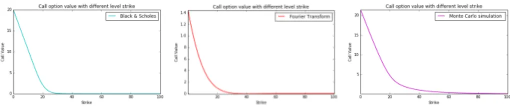
As expected, the evolution of call price at different level strike looks more closely to the Black & Scholes than Monte Carlo simulation.
5. Conclusion
Figure 2: The graphs display the relation ship between call value and strike under different models B&S, SVJJ and M.C simulation.
same time prices for about 210 strikes, while Monte Carlo simulations provide only single strike price. Therefore, all the analyzes performed show that Fourier transform pricing option under SVJJ model is versatile enough to describe pre-cisely the value of call option since they are usually traded near-the-money. For this reason, we strongly recommend the solution techniques FFT as a flexible and promising framework to be applied at general derivative security pricing problem and it is not only limited to SVJJ case.
References
[1] G. Bakshi, C. Cao and Z. Chen, Empirical performance of alternative option pricing models,J. Finance,52(1997), 2003-2049.
[2] G. Bakshi and Z. Chen, An alternative valuation model for contingent claims,J. Finance,81 (1997), 123-165.
[3] D. Bates, Jump and stochastic volatility: Exchange rate processes implicit in deutsch mark in options, In: Review of Financial Studies, (1996), 637-659.
[4] F. Black and M. Scholes, The pricing of options and corporate liabilities,
J. Political. Economy.,81 (1973), 637-659.
[5] P. Carr and D.B. Maden, Option valuation using the fast Fourier trans-form,J. Comp. Fin.,2 (1999), 61-73.
[6] D. Duffie, J. Pan and K. Singleton, Tranform analysis and asset pricing for affine jump diffusions,Econometrica, 68, No 6 (2000), 1343-1376. [7] W. Gentleman, G. Sande, Fast Fourier transform for fun and profit, In:
[8] J. Gill-Palaez, Note on the inversion theorem, Biometrika, 38 (1951), 481-482.
[9] F.B. Hanson, Applied Stochastic Processes and Control for Jump-Diffusions: Modeling, Analysis and Computation, Philadelphia (2006). [10] S. Heston, A closed-form solution for option with stochastic volatility with
applications to bond and currency options, In: Review of Financial Study
(1993), 337-343.
[11] R.A. Jarrow and E.R. Rosenfeld, Jump risks and the inter-temporal capital asset pricing model, J. Business,57(1984), 337-351.
[12] R.C. Merton, Theory of rational option pricing, J. Economy. Mgmt., 4 (1973), 141-183.
[13] R.C. Merton, Option pricing when underlying stock returns are discontin-uous, J. Financial Economics,3 (1981), 125-144.
[14] E. Stein and J. Stein, Stock price distributions with stochastic volatility, in: Review of Financial Studies (1991), 727-752.