ISSN: 1311-1728 (printed version); ISSN: 1314-8060 (on-line version) doi:http://dx.doi.org/10.12732/ijam.v30i1.2
INTERIOR-POINT METHODS FOR P∗(κ)-LINEAR COMPLEMENTARITY PROBLEM BASED ON
GENERALIZED TRIGONOMETRIC BARRIER FUNCTION
M. El Ghami1§, G.Q. Wang2 1Mathematics Section
Faculty of Education and Arts Nord University
Nesna 8700, NORWAY
2College of Fundamental Studies
Shanghai University of Engineering Science Shanghai, 201620, P.R. CHINA
Abstract: Recently, M. Bouafoa, et al. [3] investigated a new kernel function which differs from the self-regular kernel functions. The kernel function has a trigonometric Barrier Term. In this paper we generalize the analysis presented in the above paper for P∗(κ) Linear Complementarity Problems (LCPs). It is shown that the iteration bound for primal-dual large-update and small-update interior-point methods based on this function is as good as the currently best known iteration bounds for these type methods. The analysis for LCPs deviates significantly from the analysis for linear optimization. Several new tools and techniques are derived in this paper.
AMS Subject Classification: 65K05, 90C33
Key Words: interior-point, kernel function, primal-dual method, large up-date, small upup-date, linear complementarity problem
Received: October 18, 2016 c 2017 Academic Publications
1. Introduction
In this paper we consider the following linear complementarity problem:
s = M x+q,
xs = 0, (1)
x, s ≥ 0,
where M ∈ Rn×n is a P∗(κ) matrix and q, x, s are vectors of Rn, and xs
denotes the componentwise product (Hadamard product) of vectors x and s. Linear complementarity problems have many applications in mathematical pro-gramming and equilibrium problems. Indeed, it is known that by exploiting the first-order optimality conditions of the optimization problem, any differentiable convex quadratic program can be formulated into a monotone linear comple-mentarity problem, i.e. P∗(0)LCP, and vice versa [18]. Variational inequality problems are widely used in the study of equilibrium in economics, transporta-tion planning, and game theory, and have a close connectransporta-tion to the LCP s. The reader can refer to Section 5.9 in [6] for the basic theory, algorithms, and applications.
The primal-dual IP M for linear optimization (LO) problems was first in-troduced in [11, 14] and extended to various class of problems, e.g. [4, 16]. Kojima et al. [11] and Monteiro et al. [14] first proved the polynomial com-putational complexity of the algorithm for LO problem independently, and since then many other algorithms have been developed based on the primal-dual strategy. Kojima et al. [12] proved the existence of the central path for any P∗(κ) LCP, generalized the primal-dual interior-point algorithm in [11] to
P∗(κ) LCP and proved the same complexity results. Miao [13] extended the Mizuno-Todd-Ye predictor-corrector method to P∗(κ) LCP s. His algorithm uses the l2-neighborhood of the central path and has O((1 +κ)√nL)
itera-tion complexity. Ill´es and Nagy [10] give a version of the Mizuno-Todd-Ye predictor-corrector interior point algorithm for the P∗(κ) LCP and show that the complexity of the algorithm is O(1 +κ)32 √nL
. They choose τ and τ′
neighborhood parameters in such a way that at each iteration a predictor step is followed by one corrector step. For larger value of κ the values of τ and τ′
decrease fast, therefore the constant in the complexity results is increasing. Most of the polynomial-time interior point algorithms forLOare based on the use of the logarithmic barrier function [11, 17]. Peng et al. [16] introduced self-regular barrier functions for primal-dual interior-point methods (IP M s) for
and also extended to P∗(κ) LCP s. Recently in [2, 7] the authors proposed a new primal-dual IP M for LO based on a new class of kernel functions which are not logarithmic and not necessarily self-regular barrier functions.
In this paper we propose a new large-update primal-dualIP M which gener-alizes the results obtained in [7] toP∗(κ)LCP s. We use a new search direction based on kernel functions which are neither logarithmic nor self-regular barrier. The new analysis which is derived in this paper is different from the one used in early papers [10, 12, 13, 16]. Furthermore, our analysis provides a simpler way to analyze primal dualIP M s.
We use the following notational conventions. Throughout the paper, k·k denotes the 2-norm of a vector. The nonnegative orthant and positive orthant are denoted as Rn+ and Rn++, respectively. Ifz∈Rn+ and f :R+→R+, then f(z) denotes the vector inRn+ whose i-th component isf(zi), with 1≤i≤n. Finally, for x ∈ Rn, X = diag (x) is the diagonal matrix from vector x, and
J ={1,2, ..., n} is the index set.
This paper is organized as follows. In Section 2 we recall basic concepts and the notion of the central path. In Section 3 we review known results relevant for the development of the analysis. Section 4 contains new results to compute the feasible step size and the study of the amount of decrease of the proximity function during an inner iteration. Section 5 combiners the results from Section 3 and the derived results in Section 4 to show the bound for the total number of iterations of the algorithm. Finally, concluding remarks are given in Section 6.
2. Preliminaries
In this section we introduce the definition of P∗(κ) matrix and its proprieties, [12].
Definition 1. LetY be an open convex subset ofRnandκ≥0. A matrix
M ∈Rn×n is called a P∗(κ)-matrix on Y if and only if (1 + 4κ) X
i∈J+(x)
xi(M x)i+
X
i∈J−(x)
xi(M x)i≥0,
for all x∈Y, where
J+(x) ={i∈J :xi(M x)i ≥0} andJ−(x) ={i∈J :xi(M x)i <0}.
Note that the class of P∗-matrices is the union of all P∗(κ)-matrices for
κ≥0, and contains the class of positive semi-definite matrices, i.e. symmetric matricesM satisfyingPi∈Jxi(M x)i ≥0 for allx∈Rn, by choosingκ= 0. The class of P∗ matrices also contains matrices with all positive principal minors. In the following we recall some results which are essential in our analysis.
Proposition 2. [Lemma 4.1 in [12]] IfM ∈Rn×nis a P∗ matrix, then M′ =
−M I
S X
is a nonsingular matrix for any positive diagonal matrices X,S ∈Rn×n.
We use the following corollary of Proposition 2 to prove that the modified Newton system has a unique solution.
Corollary 3. Let M ∈Rn×n be aP∗ matrix and x,s ∈Rn++. Then for all a∈Rn the system
−M△x+△s = 0, S△x+X△s = a,
has a unique solution (△x,△s).
The basic idea of primal-dual interior-point methods is to replace the second equation in (1) by the nonlinear equationxs=µe, whereeis the all-one vector, and µ >0. Thus we have the following parameterized system:
s = M x+q,
xs = µe, (2)
x ≥ 0, s≥0,
whereµ >0. We assume that there exists strictly positivex andsthat satisfy (1).
Let (x, s) be a strictly feasible point andµ >0. We define the vector
v:=
rxs
µ. (3)
Note that the pair (x, s) coincides with the µ-center (x(µ), s(µ)) if and only if
v=e.
Let Ψ(v) be a smooth, strictly convex function defined for allv >0, which is minimal at v= e, with Ψ(e) = 0. Following [1, 2, 5, 8, 16] we define search directions ∆x, ∆sby
−M∆x+ ∆s = 0,
s∆x+x∆s = −µv∇Ψ(v). (4)
SinceM is aP∗ matrix, the system (4) uniquely defines (∆x,∆s) for anyx >0 and s > 0. Note that ∆x = 0, ∆s = 0, if and only if v = e, because the right-hand sides in (4) vanish if and only if ∇Ψ(v) = 0, and this occurs if and only if v=e.
Let (x, s) be a strictly feasible point. We define the vectorp by
p:=
r x
s. (5)
Introducing the following notations
¯
M :=P M P and P := diag (p), V := diag (v) where v=
rxs µ,
and
dx :=
v∆x
x , ds:= v∆s
s , (6)
the system (4) can be reformulated as
−M d¯ x+ds = 0,
dx+ds = −∇Ψ(v). (7)
From the solution dx and ds, the vectors ∆x and ∆s can be computed from (6).
Note that the vectorsdx andds are not orthogonal. So our analysis in this paper will deviate significantly from the analysis used forLO in [7].
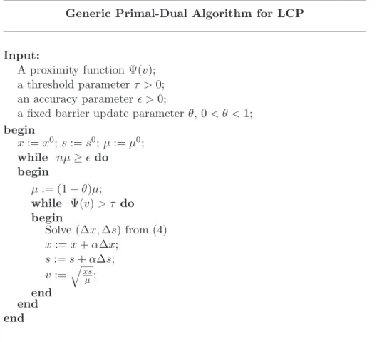
Generic Primal-Dual Algorithm for LCP
Input:
A proximity function Ψ(v); a threshold parameter τ >0; an accuracy parameter ǫ >0;
a fixed barrier update parameter θ,0< θ <1;
begin
x:=x0; s:=s0;µ:=µ0;
while nµ≥ǫdo begin
µ:= (1−θ)µ;
while Ψ(v)> τ do begin
Solve (∆x,∆s) from (4)
x:=x+α∆x;
s:=s+α∆s;
v:=qxsµ;
end end end
Figure 1: The generic primal-dual interior-point algorithm for LCP
The inner while loop in the algorithm is calledinner iteration and the outer while loop outer iteration. So each outer iteration consists of an update of the barrier parameter and a sequence of one or more inner iterations. We assume that (1) is strictly feasible, and the starting point x0, s0is strictly feasible for (1). Chooseτ andv0 =qx0s0
µ0 initial strictly feasible point such that Ψ v0
≤τ
and construct a new pair (x+, s+) with
x+ =x+α△x s+=s+α△s. (8)
If necessary, we repeat the procedure until we find iterates such that Ψ(v) no longer exceed the threshold value τ, which means that the iterates are in a small enough neighborhood of (x(µ), s(µ)). Then µ is again reduced by the factor 1−θ and we apply the same procedure targeting at the new µ-centers. This process is repeated untilµis small enough, i.e. untilnµ≤ǫ. At this stage we have found an ǫ-solution of (1). Just as in the LO case, the parameters
τ, θ, and the step size α should be chosen in such a way that the algorithm is ‘optimized’ in the sense that the number of iterations required by the algorithm is as small as possible. Obviously, the resulting iteration bound will depend on the kernel function underlying the algorithm, and our main task becomes to find a kernel function that minimizes the iteration bound.
Figure 1 gives some examples of kernel functions that have been analyzed in [8] with the complexity results for the corresponding algorithms for large-update methods. For small-update interior-point methods the complexity results ob-tained in [8] is as good as the currently best known iteration bounds for these type methods methods namely: O (1 + 2κ)√nlognǫ.
The aim of this paper is to investigate a new kernel function studied first in linear optimization case in [3], namely
ψ(t) = t
2−1
2 +
4
pπ(tan
p(h(t))
−1), (9)
with h(t) = π
2t+2, and p ≥ 2 and to show that the interior-point methods
for linear complementarity based on these function have favorable complexity results.
Note that the growth term of our kernel function is quadratic as all kernel functions in Table 1. However, this function (9) deviates from all other ker-nel functions [8] since its barrier term is trigonometric as pπ4 (tanp(h(t))−1). In order to study the new kernel function, several new arguments had to be developed for the analysis.
3. Properties of the New Proximity Function
i kernel functionsψi Large-update
1 t2−1
2 −logt O (1 + 2κ)nlog n
ǫ
2 t2
−1 2 +
t1−q −1 q(q−1) −
q−1
q (t−1) O
(1 + 2κ)qnq+12q logn
ǫ
3 12 t−1t
2
O(1 + 2κ)n23logn
ǫ
4 t2−1 2 +e
1
t−1−1 O (1 + 2κ)√n log2nlogn ǫ
5 t2−1 2 −
Rt 1e
1
ξ−1dξ O (1 + 2κ)√n log2nlogn ǫ
6 t2−1 2 +
t1−q −1
q−1 , q >1 O
(1 + 2κ)qnq+12q logn
ǫ
7 t−1 + t1−q −1
q−1 , q >1 O (1 + 2κ)qnlog n ǫ
8 t2−1 2 +
6 πtan
π(1
−t) 4t+2
O(1 + 2κ)n34logn
ǫ
Table 1: Examples of kernel functions studied in early paper [8] with complexity results for large-update.
3.1. Some Technical Results
The first three derivatives ofψ are given by
ψ′(t) = t+4h′(t)
π sec
2(h(t)) tanp−1(h(t)), (10)
ψ′′(t) = 1 + 4
π sec
2(h(t))g(t), (11)
ψ′′′(t) = 4
πsec
2(h(t)) k(t)h′(t)3+r(t)h′′(t)h′(t)h′′′(t) (12)
+ tanp−1(h(t))h′′′(t), (13) with
g(t) := (p−1) tanp−2(h(t)) + (p+ 1) tanp(h(t))h′(t)2 + h′′(t) tanp−1(h(t)),
and
r(t) := 3 (p−1) tanp−2(h(t)) + 3 (p+ 1) tanp(h(t)), (14)
and the first three derivatives of h are given by
h′(t) = −π
2 (t+ 1)2; h
′′(t) = π
(t+ 1)3; h
′′′(t) = −3π
(t+ 1)4.
The next lemma serves to prove that the new kernel function (9) is eligible.
Lemma 4(Lemma 3.2 in [3]). Letψbe as defined in (9) andt >0. Then,
ψ′′(t) > 1, (15-a)
tψ′′(t) +ψ′(t) > 0, (15-b)
tψ′′(t)−ψ′(t) > 0, (15-c)
and ψ′′′(t) < 0. (15-d)
It follows that ψ(1) = ψ′(1) = 0 andψ′′(t) ≥0, proving that ψ is defined by ψ′′(t),
ψ(t) =
Z t
1 Z ξ
1
ψ′′(ζ)dζdξ. (16)
The second property (15-b) in Lemma 4 is related to Definition 2.1.1 and Lemma 2.1.2 in [16]. This property is equivalent to convexity of the composed function
z 7→ ψ(ez) and this holds if and only if ψ(√t1t2) ≤ 12(ψ(t1) +ψ(t2)) for any t1, t2 ≥ 0. Following [1], we therefore say that ψ is exponentially convex, or shortly,e-convex, whenevert >0.
Lemma 5. Letψ be as defined in (9), one has ψ(t)< 1
2ψ
′′(1) (t−1)2, if t >1.
Proof. By Taylor’s theorem and ψ(1) =ψ′(1) = 0,we obtain
ψ(t) = 1 2ψ
′′(1) (t−1)2
+1 6ψ
′′′(ξ) (ξ−1)3,
where 1< ξ < tif t >1. Since ψ′′′(ξ)<0,the lemma follows.
Proof. Definingg(t) :=tψ′(t)−ψ(t) one has g(1) = 0 andg′(t) =tψ′′(t)≥ 0.Hence g(t)≥0 and the lemma follows.
Following [2], we now introduce a norm-based proximity measure δ(v), ac-cording to
δ(v) := 12kψ′(v)k= 1 2
v u u t
n
X
i=1
ψ′(vi)2= 1
2kdx+dsk, (17)
in terms of Ψ(v). Since Ψ(v) is strictly convex and attains its minimal value zero at v=e, we have
Ψ (v) = 0 ⇔ δ(v) = 0 ⇔ v=e.
3.2. Relations between Proximity Measure and Norm-Based Proximity Measure
For the analysis of the algorithm in Section 4 we need to establish relations between Ψ(v) and δ(v). A curial observation is that the inverse function of
ψ(t), for t≥1, plays an important role in this relation.
The next theorem, which is one of main results in [2], gives a lower bound on δ(v) in term of Ψ(v). This is due to the fact that ψ(t) satisfies (15-d). The theorem is a special case of Theorem 4.9 in [2], and is therefore stated without proof.
We denote by ̺ : [0,∞) → [1,∞) and ρ : [0,∞) → (0,1] the inverse functions of ψ(t) for t≥1,and −12ψ′(t) for t≤1, respectively. In other words,
s=ψ(t) ⇔ t=̺(s), t≥1, (18)
s=−12ψ′(t) ⇔ t=ρ(s), t≤1. (19)
Theorem 7 (Theorem 4.9 in [2]). Let̺ be as defined in (18). One has δ(v) ≥ 12ψ′(̺ (Ψ(v))).
Corollary 8. Let ̺ be as defined in (18). Thus we have δ(v) ≥ Ψ(v)
2̺(Ψ(v)).
δ(v)≥ ψ(̺(Ψ(v))) 2̺(Ψ(v)) =
Ψ(v) 2̺(Ψ(v)). This proves the corollary.
Theorem 9. If Ψ(v)≥1, then δ(v)≥ 1
6Ψ
1
2. (20)
Proof. The inverse function of ψ(t) for t ∈[1,∞) is obtained by solving t
from
ψ(t) = t
2−1
2 +
4
pπ
tanp
π
2t+ 2
−1
=s, t≥1.
We derive an upper bound fort, as this suffices for our goal. One has from (16) and ψ′′(t)≥1,
s=ψ(t) =
Z t
1 Z ξ
1
ψ′′(ζ)dζdξ≥ Z t
1 Z ξ
1
dζdξ= 1 2(t−1)
2,
which implies
t=̺(s)≤1 +√2s. (21)
Assuming s≥1,we get t=̺(s) ≤√s+√2s≤3s12.Omitting the argument
v, and assuming Ψ(v)≥1, we have̺(Ψ(v))≤3Ψ(v)12.Now, using Corollary 8,
we have
δ(v)≥ Ψ(v) 2̺(Ψ(v)) ≥
1 6Ψ(v)
1 2.
This proves the lemma.
Note that if Ψ(v)≥1,substitution in (20) gives
δ(v) ≥ 1
6. (22)
3.3. Growth Behavior of the Barrier Function
Note that at the start of each outer iteration of the algorithm, just before the update of µ with the factor 1−θ, we have Ψ(v) ≤ τ. Due to the update of
during the course of the algorithm the largest values of Ψ(v) occur just after the updates of µ. In this section we derive an estimate for the effect of aµ-update on the value of Ψ(v). We start with an important theorem which is valid for all kernel functionsψ(t) that are strictly convex (15-a), and satisfies (15-c).
Theorem 10 (Theorem 3.2 in [2]). Let̺: [0,∞)→[1,∞) be the inverse function ofψon [0,∞).Then for any positive vector vand anyβ >1 we have:
Ψ(βv)≤nψ
β̺
Ψ(v)
n
. (23)
Corollary 11. Let0< θ <1 andv+ = √1v−θ.Then
Ψ(v+)≤nψ ̺
Ψ(v)
n
√
1−θ
. (24)
Proof. Substitution ofβ = √1
1−θ into (23), the corollary is proved.
Suppose that the barrier update parameter θ and threshold value τ are given. According to the algorithm, at the start of each outer iteration we have Ψ(v) ≤ τ.By Theorem 10, after each µ-update the growth of Ψ(v) is limited by (24). Therefore we define
L=L(n, θ, τ) :=nψ ̺
τ n
√
1−θ !
. (25)
Obviously,Lis an upper bound of Ψ(v+), the value of Ψ(v) after theµ-update.
4. Analysis of the Algorithm
In this section, we show how to compute a feasible step sizeαof a Newton step with the decrease of the barrier function. Since dx and ds, are not orthogonal the analysis in this paper is different from that of LO case. After a damped step, with step sizeα, using (3) and (6) we have
x+ =x+α∆x= x
v(v+αdx), s+=s+α∆s= s
v(v+αds).
Thus we obtain
v+2 = x+s+
In the sequel we use the following notation:
ν := min
i∈J vi, δ:=δ(v), σ+:=
X
i∈J+
dxidsi, σ−:=− X
i∈J−
dxidsi. (27)
Since M is aP∗(κ) matrix, we have
(1 + 4κ) X i∈J+
∆xi(M∆x)i+
X
i∈J−
∆xi(M∆s)i ≥0,
where J+={i∈J : ∆xi(M∆x)i ≥0}, J−=J−J+. Using the first equation
in (4) we have for ∆x∈Rn,M∆x= ∆s, and (1 + 4κ) X
i∈J+
∆xi∆si+
X
i∈J−
∆xi∆si ≥0.
From (6) it follows that dxds= v
2∆x∆s
xs =
∆x∆s
µ withµ >0,and
(1 + 4κ)X i∈J+
dxidsi+ X
i∈J−
dxidsi = (1 + 4κ)σ+−σ−≥0. (28)
The next lemma gives an upper bound of σ+ and σ−.
Lemma 12. One has
σ+≤δ2, and σ−≤(1 + 4κ)δ2.
Proof. By the definition ofσ+,σ− andδ, we have
σ+= X
i∈J+
dxidsi ≤
1 4
X
i∈J+
(dxi+dsi) 2
≤ 14X
i∈J
(dxi+dsi) 2
= 1
4kdxi+dsik 2 =δ2.
Since M is aP∗(κ) matrix, using (28), we get
(1 + 4κ)σ+−σ−≥0.
Thus
σ−≤(1 + 4κ)σ+≤(1 + 4κ)δ2.
This proves the lemma.
Lemma 13. One has
n
X
i=1
d2xi+d2si ≤4 (1 + 2κ)δ2, kdxk ≤2
√
1 + 2κ δ,
and kdsk ≤2
√
1 + 2κ δ.
Proof. From the definitions (17) and (27), we have
δ= 1
2kdx+dsk, and
X
j∈J
dxidsi =σ+−σ−,
then
2δ=kdx+dsk=
v u u t n X i=1
(dxi+dsi) 2 = v u u t n X i=1 d2
xi +d 2
si
+ 2 (σ+−σ−).
Using (28), and Lemma 12, we get
2δ ≥ v u u t n X i=1 d2
xi+d 2 si + 2 1
1 + 4κσ−−σ− = v u u t n X i=1 d2
xi+d 2
si
−1 + 48κκσ−.
Then, we get
4δ2+ 8κ
1 + 4κσ− ≥
n
X
i=1 d2x
i+d 2
si
.
Using again Lemma 12, we have
4 (1 + 2κ)δ2 ≥4δ2+ 8κ
1 + 4κσ−≥
n
X
i=1
d2xi+d2si.
Thus
kdxk ≤
v u u t n X i=1 d2
xi+d 2
si
≤2√1 + 2κ δ.
Using the same argument we can prove that
kdsk ≤2
√
Thus the lemma follows.
Our aim is to find an upper bound for
f(α) := Ψ (v+)−Ψ (v) := Ψ p
(v+αdx) (v+αds)−Ψ (v),
where Ψ :Rn→Ris given by Ψ(v) =
n
X
i=1
ψ(vi). (29)
To do this, the next four technical lemmas are needed. It is clear that f(α) is not necessarily convex in α. To simplify the analysis we use a convex upper bound for f(α). Such a bound is obtained by using that ψ(t) satisfies the condition (15-b). Hence, ψ(t) ise-convex. This implies
Ψ (v+) = Ψ p
(v+αdx) (v+αds)≤ 12[Ψ (v+αdx) + Ψ (v+αds)].
Thus we havef(α)≤f1(α), where
f1(α) := 12[Ψ (v+αdx) + Ψ (v+αds)]−Ψ (v)
is a convex function of α, since Ψ(v) is convex. Obviously, f(0) = f1(0) = 0.
Taking the derivative off1(α) to α, we get
f1′(α) = 12 n
X
i=1
ψ′(vi+αdxi)dxi+ψ′(vi+αdsi)dsi
.
This gives, using last equation in (7) and (17),
f1′(0) = 12∇Ψ(v)T (dx+ds) =−21∇Ψ(v)T∇Ψ(v) =−2δ(v)2. (30)
Differentiating once more, we obtain
f1′′(α) = 12 n
X
i=1
ψ′′(vi+αdxi)dx2i +ψ′′(vi+αdsi)ds2i
. (31)
From this stage on we can apply word-by-word the same arguments as in [8] to obtain the following results that are therefore stated without proof.
The following lemma gives an upper bound off1(α) in terms ofδandψ′′(t).
Lemma 14 (Lemma 4.3 in [8]). One has
Putting
δκ:=
√
1 + 2κ δ, (32)
we have
f1′′(α)≤2δκ2ψ′′(ν−2αδκ), (33)
Sincef1(α) is convex, we will have f1′(α)≤0 for all αless than or equal to the
value where f1(α) is minimal, and vice versa. In this respect the next result is
important.
Lemma 15 (Lemma 4.4 in [8]). One has f′
1(α) ≤ 0 if α satisfies the inequality
−ψ′(ν−2αδκ) +ψ′(ν)≤ 2δκ
(1 + 2κ). (34)
The next lemma uses the inverse functionρ: [0,∞)→(0,1] of −12ψ′(t) for
t∈(0,1], as defined in (19).
Lemma 16 (Lemma 4.5 in [8]). The largest value of the step size α satisfying (33) is given by
¯
α:= 1 2δκ
ρ(δ)−ρ
1 +√1 + 2κ
1 + 2κ δκ
. (35)
Moreover
¯
α≥ 1
(1 + 2κ)ψ′′ρ1+√1+2κ 1+2κ δκ
. (36)
For future use we define
e
α:= 1
(1 + 2κ)ψ′′ρ1+√1+2κ
1+2κ δκ
, (37)
as the default step size. By Lemma 16 this step αe satisfies (34). By (36) we have ¯α≥α˜. We recall without proof the following lemma from [15].
Lemma 17(Lemma 3.12 in [15]). Leth(t)be a twice differentiable convex function with h(0) = 0, h′(0) <0 and let h(t) attain its (global) minimum at t∗ >0. Ifh′′(t) is increasing fort∈[0, t∗]then
h(t)≤ th′(0)
2 , 0≤t≤t
Lemma 18 (Lemma 10 in [9]). If the step sizeα satisfies (34) then
f(α)≤ −α δ2. (38)
Theorem 19. Letρ be defined in (19) andαe in (37). Then
f(αe)≤ − δ
2
(1 + 2κ)ψ′′ρ1+√√1+2κ 1+2κ δ
≤ − δ
p
1+p
1320p(1 + 2κ). (39)
Proof. By combining (36) in Lemma 16 and results in Lemma 18, using also (32).Thus the first inequality in (39) follows.
To obtain the inverse function t=ρ(s) of−12ψ′(t) for t∈(0,1], we need to
solve tfrom the equation
−
t+4h′(t)
π sec
2(h(t)) tanp−1(h(t))
=
−t+ 4h′(t)
π csc
2(h(t)) tanp+1(h(t))
= 2s.
This implies,
csc2(h(t)) tanp+1(h(t)) = −π
4h′(t)(2s+t).
Fort≤1, we get 2π(4t+1)π 2 (2s+t)≤2 (2s+ 1).Hence, putting
t=ρ
1 +√1 + 2κ √
1 + 2κ δ
,
which is equivalent to 2(1+
√ 1+2κ)
√
1+2κ δ = −ψ′(t). Using that
1+√√1+2κ
1+2κ ≤2 for all
κ≥0, and sin2(h(t))≤1 we get
tan(h(t))≤(8δ+ 2)1+1p. (40)
Since sec2(h(t)) = 1 + tan2(h(t)), By (40), thus we have
tan2(h(t))≤(8δ+ 2)1+2p, tanp−2(h(t))≤(8δ+ 2) p−2 1+p,
tanp−1(h(t))≤(8δ+ 2)p1+−1p and tanp(h(t))≤(8δ+ 2) p
Since h′′(t) = 8π
8(t+1)3 ≤ 3π
4 , and h′(t)2 = 4
π2
16(2t+1)4 ≤
π2
4 for all 0 ≤t ≤1, and
using also (8δ+ 2)≥1 this implies
ψ′′(t)≤
1 + 4
π2
2pπ 2
4 +π
(8δ+ 2)p1++2p = (9 + 4pπ) (8δ+ 2) p+2 1+p.
By (37), thus we have
e
α = 1
(1 + 2κ)ψ′′ρ1+√√1+2κ 1+2κ δ
≥ 1
(1 + 2κ) (9 + 4pπ) (8δ+ 2)p1++2p .
Also using (22) (i.e., 6δ ≥1) and p≥2 we get,
e
α ≥ 1
(1 + 2κ) (9 + 4pπ) (8δ+ 12δ)p1++2p
= 1
(1 + 2κ) (9 + 4pπ) (20δ)p1++2p
≥ 1
1320p(1 + 2κ)δp1++2p .
Hence
f(αe)≤ − δ
2
1320p(1 + 2κ)δp1++2p
=− δ
p
1+p
1320p(1 + 2κ).
Thus the theorem follows. Substitution in (20) gives
f(˜α)≤ − δ
p
1+p
1320p(1 + 2κ) ≤ −
Ψ2(1+pp)
1320p(6)1+pp(1 + 2κ)
≤ − Ψ p
2(1+p)
7920p(1 + 2κ).
5. Iteration Complexity
5.1. Upper Bound for the Total Number of Iterations
Let K denote the number of inner iterations. An upper bound for the total number of iterations is obtained by multiplying (the upper bound for) the num-berK by the number of barrier parameter updates, which is bounded above by
1
θlog n
ǫ (cf. [17] Lemma II.17, page 116).
Lemma 20 (Proposition 2.2 in [15]). Let t0, t1,· · · , tK be a sequence of
positive numbers such that
tk+1≤tk−κt1−k γ, k= 0,1,· · · , K−1,
whereκ >0 and 0< γ≤1. Then K≤jt γ
0
κγ
k .
Lemma 21. If K denotes the number of inner iterations, we have
K ≤7920p(1 + 2κ) Ψ
2+p
2(1+p)
0 .
Proof. The definition of K implies ΨK−1 > τ and ΨK ≤τ and
Ψk+1≤Ψk−κ(Ψk)1−γ, k= 0,1,· · · , K−1,
with κ= 7920p(1+21 κ) and γ = 2(1+2+pp). Application of Lemma 20, with tk = Ψk yields the desired inequality.
Usingψ0 ≤L, where the number Lis as given in (25), and Lemma 21 we
obtain the following upper bound on the total number of iterations:
7920p(1 + 2κ)L 2+ p
2(1+p)
θ log
n
ǫ. (41)
5.2. Large-Update
We just established that (41) is an upper bound for the total number of itera-tions, using
ψ(t) = t
2−1
2 +
4
pπ
tanp
π
2t+ 2
−1
and (21), by substitution in (25) we obtain
L≤n
̺(τ n) √ 1−θ 2 −1 2 ≤ n
2 (1−θ)
θ+ 2
r 2τ n+ 2τ n
= θn+ 2
√
2τ n+ 2τ
2 (1−θ) .
Using (41), thus the total number of iterations is bounded above by
K θ log
n ǫ ≤
7920p(1 + 2κ)
θ2 (1−θ)2(1+2+pp)
θn+ 2√2τ n+ 2τ
2+p
2(1+p)
logn
ǫ.
A large-update methods uses τ = O(n) and θ = Θ(1). The right-hand side expression is then O
p(1 + 2κ)n
2+p
2(1+p) logn
ǫ
,as easily may be verified.
5.3. Small-Update Methods
For small-update methods one has τ = O(1) and θ= Θ√1n
. Using Lemma 5, withψ′′(1) = pπ4+8,we then obtain
L≤ n(pπ+ 8)
8
ρ τn √
1−θ−1 !2
.
Using (21), then
L≤ n(pπ+ 8)
8
1 +
q 2τ
n
√
1−θ −1 2
.
Using 1−√1−θ= θ
1+√1−θ ≤θ,this leads to
L≤ (pπ+ 8)
8 (1−θ)
θ√n+√2τ 2
.
We conclude that the total number of iterations is bounded above by
K θ log
n ǫ ≤
7920 (1 + 2κ) (pπ+ 8)2(1+2+pp)
θ(8 (1−θ))2(1+2+pp)
θ√n+√2τ
2+p
1+p
logn
ǫ.
Thus the right-hand side expression is then O (1 + 2κ)√nlogn ǫ
6. Concluding Remarks
In this paper we extended the results obtained for kernel-function-based IPMs in [3] for LO toP∗(κ) linear complementarity problems. The observation that the vectorsdx anddsare not in general orthogonal implies that the analysis in [3, 7] does not hold. The analysis in this paper is new and different from the one using for LO. Several new tools and techniques are derived in this paper. The proposed function has a trigonometric barrier term but the function is not logarithmic and not self-regular. For this parametric kernel function, we have shown that the best result of iteration bounds for large-update methods and small-update can be achieved, namelyO (1 + 2κ) logn√nlognǫ,for large-update and O (1 + 2κ)√nlogn
ǫ
for small-update methods.
The resulting iteration bounds for P∗(κ) linear complementarity problems depend on the parameterκ. Forκ= 0, the iteration bounds are the same as the bounds that were obtained in [3] for linear optimization. In our future study, we intend to generalize the primal-dual IPMs to general nonlinear symmetric cone optimization based on this parametric kernel function.
Acknowledgments
The authors would like to thank the editor and the anonymous referees for their useful comments and suggestions, which helped to improve the presen-tation of this paper. This work was supported by National Natural Science Foundation of China (No. 11471211), Shanghai Natural Science Fund Project (No. 14ZR1418900) and the Scientific Research Foundation for the Returned Overseas Chinese Scholars, State Education Ministry.
References
[1] Y.Q. Bai, M. El Ghami, and C. Roos, A new efficient large-update primal-dual interior-point method based on a finite barrier, SIAM Journal on Optimization,13, No 3 (2003), 766–782.
[2] Y.Q. Bai, M. El Ghami, and C. Roos, A comparative study of kernel functions for primal-dual interior-point algorithms in linear optimization,
SIAM Journal on Optimization,15, No 1 (2004), 101–128.
function with a trigonometric barrier term, J. of Optimization Theory and Applications, 170, No 2 (2016), 528–545; doi: 10.1007/s10957-016-0895-0. [4] E. M. Cho, Log-barrier method for two-stagequadratic stochastic
program-ming, Applied Mathematics and Computation, 164(2005), 45–69.
[5] Gyeong-Mi Cho, and Min-Kyung Kim, A new large-update interior point algorithm forP∗(κ) LCPs based on kernel functions, Applied Mathematics and Computation, 182 (2006), 1169–1183.
[6] R. Cottle, J.S. Pang, and R.E. Stone, The Linear Complementarity Prob-lem, Academic Press, Boston, 1992.
[7] M. El Ghami, Z. A. Guennoun, S. Bouali and T. Steihaug, Primal-dual interior-point methods for linear optimization based on a kernel function with trigonometric barrier term, J. of Computational and Applied Mathe-matics,236, No 15 (2012), 3613–3623.
[8] M. El Ghami, and T. Steihaug, Kernel-function based primdual al-gorithms for P∗(κ) linear complementarity problems, International J. RAIRO-Operations Research,44, No 3 (2010), 185–205.
[9] M. El Ghami, Primal-dual algorithms for P∗(κ) linear complementarity problems based on kernel-function with trigonometric barrier term, Opti-mization Theory, Decision Making, and Operations Research Applications 2013 (2013), 331–349.
[10] T. Ill´es doiand M. Nagy, The Mizuno-Todd-Ye predictor-corrector algo-rithm for sufficient matrix linear complementarity problem,Alkalmaz. Mat. Lapok 22, No 1 (2005), 41–61, doi: 10.1016/j.ejor.2005.08.031.
[11] M. Kojima, N. Megiddo, T. Noma, and A. Yoshise, A primal-dual interior point algorithm for linear programming, In: N. Megiddo (Ed.), Progress in Mathematical Programming; Interior Point Related Methods,10(1989), Springer Verlag, New York, 29–47.
[12] M. Kojima, N. Megiddo, T. Noma, and A. Yoshise, A unified Approach to Interior Point Algorithms for Linear Complementarity Problems, Volume 538 of Lecture Notes in Computer Science, Springer Verlag, Berlin, 1991.
[14] R.D.C. Monteiro and I. Adler, Interior path following primdual al-gorithms. Part I: Linear programming, Mathematical Programming, 44
(1989), 27–41.
[15] J. Peng, C. Roos, and T. Terlaky, Self-regular functions and new search directions for linear and semidefinite optimization, Mathematical Program-ming,93(2002), 129–171.
[16] J. Peng, C. Roos, and T. Terlaky, Self-Regularity: A New Paradigm for Primal-Dual Interior-Point Algorithms. Princeton University Press, 2002.
[17] C. Roos, T. Terlaky, and J.-Ph. Vial, Theory and Algorithms for Linear Optimization. An Interior-Point Approach, Springer Science, 2005.
![Table 1: Examples of kernel functions studied in early paper [8] with complexity results for large-update.](https://thumb-us.123doks.com/thumbv2/123dok_us/8107293.2149582/8.748.195.585.143.474/table-examples-kernel-functions-studied-complexity-results-update.webp)
