ISSN: 1311-1728 (printed version); ISSN: 1314-8060 (on-line version) doi:http://dx.doi.org/10.12732/ijam.v33i3.7
CONFIDENCE INTERVALS FOR THE SCALE PARAMETER OF A TWO-PARAMETER WEIBULL DISTRIBUTION: ONE
SAMPLE PROBLEM
Moustafa O.A. Abu-Shawiesh1§, Juthaphorn Sinsomboonthong2,
Ahmad M.A. Adawi3, Mohammad H. Almomani4 1 Department of Mathematics, Faculty of Science
The Hashemite University, Al-Zarqa, 13115, JORDAN
2 Department of Statistics, Faculty of Science
Kasetsart University, Bangkok, 10900, THAILAND
3 Department of Mathematics, Faculty of Science
The Hashemite University, Al-Zarqa, 13115, JORDAN
4 Department of Mathematics, Faculty of Science
The Hashemite University, Al-Zarqa, 13115, JORDAN
Abstract: The problem of interval estimating for the scale parameterθ in a two parameter Weibull distribution is addressed. The pivotal quantities whose percentiles can be used to construct confidence limits for the scale parameter
θ are derived. Therefore in this paper, an exact, asymptotic and approximate (1−α)100% confidence intervals for the scale parameterθof the two parameter Weibull distribution for the case of the one sample problem are derived. The three confidence intervals are simple and easy to compute. A Monte Carlo simulation study is performed to compare the efficiencies of the three confidence interval methods in terms of two criteria, coverage probabilities and average widths. The simulation results showed that the proposed confidence intervals perform well in terms of coverage probability and average width. Additionally, when the three methods are compared, it is found that the performance of the method depends on the value of the shape parameterβ, scale parametersθand sample sizenused. The three methods are illustrated using a real-life data set which also supported the findings of the simulation study to some extent.
Received: February 19, 2020 c 2020 Academic Publications
AMS Subject Classification: 62F10, 62F35
Key Words: confidence interval; Weibull distribution; exponential distribu-tion; normal distribudistribu-tion; asymptotics; pivotal quantity; coverage probability; average width
1. Introduction
The Weibull distribution was introduced several decades ago by Waalobi Weibull [1]. It is a flexible distribution that can encompass characteristics of several other distributions. For example, it approximates the normal distribution as the shape parameter is about 3.6 in which case the skewness become zero, [2]. Also, it becomes the exponential and Rayleigh distributions when the shape pa-rameter is equal to one and two, respectively [3]. This property has given rise to widespread applications. The Weibull distribution has many applications in statistics and other areas. For further details on applications of the Weibull distribution, we refer the readers to, for example; [4], [5], [6] and [7].
The general theory of confidence interval estimation was developed by [8] and widely used technique of constructing a confidence interval (CI) of the pa-rameter for a probability distribution is based on the pivotal quantities approach which determines what is known as an exact confidence interval as mentioned by [9] and [10]. The pivotal quantity method is valid for any sample size n as mentioned by [11], [12] and [13]. Therefore, a confidence interval (CI) can be defined as a range of values that gives the user for a sense of precise statistic estimates of the parameter, [14]. When a large sample size n is applied, an asymptotic confidence interval is mostly used to construct a sequence of the es-timator ˆθnofθwith a probability density functionf(.;θ) that is asymptotically normally distributed with meanθ and variance σn2(θ) ([15], [16], [17]).
Because of its importance, many estimation methods have been proposed for the Weibull distribution for both complete and censored samples data. Re-cently, many main estimation methods have been proposed by many authors. The most common estimation method is the maximum likelihood estimation (MLE) which has attractive efficiency properties and is asymptotically unbi-ased. The use of the proposed estimation methods depends on the area of application. For further details on the main estimation methods, we refer the readers to [18], [7], [19], [20] and [21] among others.
ap-proach. The evaluation of the efficiency for these proposed confidence intervals will be proved via conducting an extensive Monte-Carlo simulation study to compare the coverage probability (CP) and the average width (AW). Further-more, the three methods will be illustrated using a real-life data in order to demonstrate how the proposed confidence intervals can be applied in practice and support the findings of the simulation study.
The structure for the rest of this paper is organized as follows: In Section 2, materials and methods are discussed. In Section 3, the three proposed confi-dence interval methods for the scale parameter (θ) of the two parameter Weibull distribution are derived. A Monte-Carlo simulation study has been conducted in Section 4. In Section 5, a real-life data are analyzed to illustrate the imple-mentation of the methods. Finally, some concluding remarks are presented in Section 6.
2. Materials and methods
In this section, we will discuss the criteria for the efficiency comparison among the considered confidence intervals and the essential conditions for the work in this study. In addition, we will derive the pivotal quantity that will be used in this study to construct the proposed (1−α)100% confidence interval (CI) for the population mean of the one parameter exponential distribution.
2.1. Criteria for the efficiency comparison
The efficiency comparison criteria among the three estimation methods of the (1−α)100% confidence intervals are the coverage probability (CP) and the average width (AW) of the resulting confidence intervals. It is acknowledged that the CP and AW are useful criteria for evaluating the confidence intervals. Let CI=(L(X),U(X)) be a confidence interval of a parameter θ based on the dataXhaving the nominal (1−α)100% confidence level, where L(X) and U(X), respectively, are the lower and upper endpoints of this confidence interval. The following definitions provide the efficiency comparison criteria in this study:
Definition 1. The coverage probability (CP) associated with a confidence interval CI=(L(X),U(X)) for the unknown parameterθof a probability density functionf(x;θ) is measured by Pθ{θ∈(L(X), U(X))}(see [16]).
simply the difference between the upper U(X) and lower L(X) endpoints of a confidence interval CI=(L(X),U(X)). The expected length of a confidence interval CI=(L(X),U(X)) is given by Eθ(W) (see [22], [23], [24]).
2.2. Essential conditions for the study
Throughout the following discussion, the essential conditions for the work in this study are denoted by (C1)–(C3)and will be given as follows:
(C1) Let X1, X2, . . . , Xn be a random sample of size n from a population
of two parameter Weibull distribution with shape parameter β (known) and scale parameter θ such that β and θ ∈ Ω where Ω = {(β, θ) : θ < β <∞; 0 < θ < ∞}. The probability density function (pdf) of the two parameter Weibull random variable X is given by equation (1) below:
f(x;β, θ) =
β θ x
β−1 e− xβ
θ ; x >0, β >0, θ >0,
0 ; Otherwise.
(1)
The cumulative distribution function (CDF) of the two parameter Weibull distribution with shape parameter β (known) and scale parameter θ is given by equation (2) below:
F(x;β, θ) =P(X≤x) =
1−e− xβ
θ ; x≥0, β >0, θ >0,
0 ; Otherwise.
(2)
For X has two parameter Weibull distribution with shape parameter β
(known) and scale parameter θ, that is X∼W eibull(β, θβ1), we have:
(i)
µ=E(X) =θβ1Γ
1
β + 1
(3)
(ii)
σ2=V ar(X) =θ2β Γ
2
β + 1
−
Γ
1
β + 1
2!
(iii)
σ=SD(X) =pV ar(X) =
v u u tθ
2
β Γ
2
β+1
−
Γ
1
β+1
2!
=θ1β
v u u
t Γ
2
β + 1
−
Γ
1
β + 1
2!
(5)
(iv) The theoretical coefficient of variation (γ), which is a useful indica-tor, is obtained as:
γ = σ
µ = θβ1
s
Γβ2 + 1−Γβ1 + 12
θ1βΓ
1 β + 1
=
s
Γβ2 + 1−Γβ1 + 12
Γβ1 + 1
(6)
(C2) Let χ2(α
2,2n) and
χ2(1−α
2,2n), respectively, be the (
α
2)th and (1− α2)th
per-centiles points (quantiles) of the chi-square distribution with 2n degrees of freedom wheren >0.
(C3) Let Zα
2 and Z1−α2, respectively, be the (
α
2)th and (1− α2)th percentiles
points (quantiles) of the standard normal distribution, Z ∼ N(0,1), which satisfy the following relation: P(|Z|< Z1−α
2) =P(−Z1−
α
2 < Z <
Z1−α2) =P(Zα2 < Z < Z1−α2) = 1−α.
2.3. The pivotal quantity derivation for the exact and approximate methods
In this section, we will derive the pivotal quantities for the exact and approxi-mate confidence interval methods considered in this paper.
Definition 3. If Q=q(X1, X2, . . . , Xn;θ) is a random variable that is a function only of X1, X2, . . . , Xn andθ, thenQis called a pivotal quantity if its
2.3.1. The pivotal quantity derivation for the exact method
In this section, we will derive the pivotal quantity that will be used later to construct the exact (1−α)100% confidence interval (CI) for the scale parameter (θ) of the two parameters Weibull distribution with shape parameterβ(known) and scale parameterθ, that is W eibull(β, θ1β).
Definition 4. IfXi ∼f(xi;θ) and ifF(x;θ) is the cumulative distribution
function (CDF) ofXi , then 1−F(xi;θ)∼U nif orm(θ,1), and consequently for
a random sample of sizen;X1, X2, . . . , Xn; it follows that the pivotal quantity:
Q=q(X1, X2, . . . , Xn;θ) =−2 n
X
i=1
ln[1−F(xi;θ)]∼χ2(2n) (7)
(see [25], page 366).
Lemma 2.1. LetX1, X2, . . . , Xn be a collection of independent and
iden-tically distributed random variables from a Weibull distribution with shape parameter β (known) and scale parameter θ, that is Xi ∼ W eibull(β, θβ1),
and if F(x;β, θ) = 1−e−xβ/θ
is the cumulative distribution function (CDF) of Xi, then the pivotal quantity is given by Q = q(X1, X2, . . . , Xn;β, θ) =
2 θ
Pn
i=1X β
i ∼χ2(2n).
Proof. To prove this, we use Definition 4 as follows:
Q=q(X1, X2, . . . , Xn;β, θ) =−2
n
X
i=1
ln[1−F(Xi;β, θ)]
=−2
n
X
i=1
lnh1−1−e−Xiβ/θ
i
=−2
n
X
i=1
lne−Xiβ/θ
=−2
n
X
i=1
−X
β i θ =
2
θ n
X
i=1
Xiβ ∼χ2(2n). (8)
2.3.2. The pivotal quantity derivation for the approximate method
parameter (θ) of the two parameters Weibull distribution with shape parameter
β (known) and scale parameterθ, that isW eibull(β, θβ1). LetX be a random
variable from a gamma distribution with the shape and scale parameters are
β (known) and θ, respectively, that is X ∼ Gamma(β, θ). The probability density function (pdf) of the random variableXis given by equation (9) below:
f(x;β, θ) =
1
θβΓ(β) xβ−1 e −x
θ ; x >0, β >0, θ >0,
0 ; Otherwise,
(9)
where Γ(x) = The gamma function = R∞
0 tx−1e−tdt. When the shape
param-eter β = 1, the gamma distribution reduces to the one parameter exponential distribution with a scale parameter θ, that is X ∼ Exp(θ). According to [2] when X follows an exponential distribution with mean θ, that is X ∼Exp(θ), the power transformationX1β has a Weibull distribution with shape parameter β (known) and scale parameterθ. That is,
X∗ =Xβ1 ∼W eibull(β, θβ1). (10)
According to [26], the use of β = 3.6 makes a good approximation to a normal curve, then X∗ = X1/3.6 is approximately normally distributed with mean, variance and standard deviation that can be given as follows:
µX∗ =E(X∗) =E(X
1
β) =θ
1
βΓ(1 + 1 β)
=θ31.6Γ(1 + 1
3.6) =θ
1 3.6Γ
4.6 3.6
= 0.90111θ31.6, (11)
σX2∗ =V ar(X∗) =V ar(X
1
β) =θ
2
β
"
Γ
1 + 2
β − Γ
1 + 1
β
2#
=θ32.6 "
Γ
1 + 2 3.6
−
Γ
1 + 1 3.6
2#
=θ32.6 "
Γ
5.6 3.6
−
Γ
4.6 3.6
2#
=θ32.6 h
0.88929−(0.90111)2i= 0.07729θ32.6, (12)
σX∗ =SD(X∗) =
q
σ2X∗ =
q
0.07729θ32.6 = 0.27801θ 1
that is,
X∗ =X31.6 ∼N
0.90111θ31.6,0.07729θ 2 3.6
, (14)
approximately as suggested by [26], and therefore the sampling distribution of the sample mean (X∗) for the power transformed data which given as follows:
X∗ =
Pn
i=1Xi∗ n
=
X∗ 1 =X
1/3.6 1
+X∗ 2 =X
1/3.6 2
+· · ·+X∗ n=X
1/3.6 n
n , (15)
will be approximately normally distributed with mean, variance and standard deviation that can be given as follows:
µX∗ =E(X∗) =µX∗ =E(X
1
β) =θ1βΓ(1 + 1
β) = 0.90111θ
1
3.6, (16)
σ2X∗ =V ar(X ∗
) = σ
2 X∗
n =
0.07729θ32.6
n , (17)
σX∗ =SD(X∗) =
q
σ2 X∗ =
σX∗
√n = 0.27801θ
1 3.6
√n , (18)
that is,
X∗ =
Pn
i=1Xi∗
n ∼N 0.90111θ
1
3.6,0.07729θ 2 3.6
n
!
. (19)
Based on the above results, we can modify the result of the central limit theorem regarding the sampling distribution of the sample mean X∗ for the
quantity Z = X−µX
σX ∼ N(0,1) using the suggested power transformation.
The modified Z∗ using the power transformation X∗ =X1/3.6 is given as fol-lows:
Z∗ = X
∗
−µX∗ σX∗
= X
∗
−0.90111θ31.6
0.27801θ31.6
√ n
= √
nX∗−0.90111θ31.6
0.27801θ31.6 ∼
N(0,1). (20)
3. The confidence intervals for the scale parameter of the Weibull distribution
In this section, for 0< α <1, the following three methods of (1−α)100% con-fidence interval are studied for the efficiency comparisons. They are the three confidence interval methods for the scale parameter (θ) of the two parameters Weibull distribution with shape parameter β (known) and scale parameter θ, namely, the exact method, the asymptotic method and the normal approxima-tion confidence interval method.
3.1. The exact confidence interval for the scale parameter of the Weibull distribution
In this section, we will obtain the (1−α)100% exact confidence interval for the scale parameter (θ) of the two parameters Weibull distribution with shape parameterβ (known) and scale parameter θ.
Lemma 3.1. LetX1, X2, . . . , Xn be a collection of independent and iden-tically distributed random variables from a Weibull distribution with shape parameterβ (known) and scale parameterθ, that isXi ∼W eibull(β, θβ1), then
by using the pivotal quantityQ=q(X1, X2, . . . , Xn;β, θ) = 2θPni=1Xiβ ∼χ2(2n),
the(1−α)100%exact confidence interval for the scale parameter (θ) of the two parameters Weibull distribution with shape parameter β (known) and scale parameterθ will be given byCIExact=
2Pni=1Xiβ χ2
(1−α/2,2n)
,2
Pn i=1X
β i χ2
(α/2,2n)
.
Proof. To prove this, we need to consider the significance level α based on the relation given in condition (C2) where χ2(α/2,2n) and χ2(1−α/2,2n) are hold by this condition, then the (1−α)100% exact confidence interval for the scale parameter (θ) of the two parameters Weibull distribution with shape parameter
β (known) and scale parameterθ can be derived as follows:
Pχ2(α/2,2n)< Q < χ2(1−α/2,2n)= 1−α,
P χ2(α/2,2n)< 2 θ
n
X
i=1
Xiβ < χ2(1−α/2,2n)
!
= 1−α,
P χ
2 (α/2,2n)
2Pn
i=1X β i
< 1 θ <
χ2(1−α/2,2n)
2Pn
i=1X β i
!
P 2
Pn
i=1X β i
χ2(1−α/2,2n) < θ <
2Pn
i=1X β i χ2(α/2,2n)
!
= 1−α. (21)
Hence, the (1−α)100% exact confidence interval for the scale parameter
(θ) is given byCIExact =
2Pni=1Xiβ χ2
(1−α/2,2n)
,2
Pn i=1X
β i χ2
(α/2,2n)
.
3.2. The asymptotic confidence interval for the scale parameter of the Weibull distribution
An asymptotic confidence interval is valid only for a sufficiently large sample size (n). This confidence interval is based on a pivotal quantity given by reduced normal random variableZ= θˆ−θ
σθˆ ∼N(0,1) asn→ ∞where ˆθis the maximum
likelihood estimator (MLE) for the scale parameter (θ) and σθˆ is the standard
error of ˆθ. Therefore we need to derive both ˆθ andσθˆ.
Lemma 3.2. LetX1, X2, . . . , Xn be a collection of independent and
iden-tically distributed random variables from a Weibull distribution with shape parameter β (known) and scale parameter θ, that is Xi ∼ W eibull(β, θ
1
β),
then the maximum likelihood estimator (MLE) of the scale parameter (θ) is ˆ
θ=
Pn i=1Xiβ
n .
Proof.
f(x;β, θ) =
β θ x
β−1 e− xβ
θ ; x >0, β >0, θ >0,
0 ; Otherwise,
L(β, θ) =
n
Y
i=1
f(xi;β, θ)
= n Y i=1 β θ x
β−1 i e −x β i θ = β θ n n Y i=1
xβi−1 e−
Pn
i x β i θ ,
lnL(β, θ) = ln
β θ n n Y i=1
xβi−1 e−
Pn
=nlnβ−nlnθ+ (β−1)
n
X
i=1
lnxi −
Pn
i x β i θ ,
dlnL(β, θ)
dθ = 0→
−n θ + Pn i x β i θ2 = 0,
−nθ+Pn
i x β i
θ2 = 0→ −nθ+ n
X
i
xβi = 0,
ˆ
θ=
Pn
i=1xβi
n . (22)
Lemma 3.3. LetX1, X2, . . . , Xn be a collection of independent and iden-tically distributed random variables from a Weibull distribution with shape parameter β (known) and scale parameter θ, that is Xi ∼ W eibull(β, θβ1),
then the maximum likelihood estimator (MLE) of the scale parameter (θ) is ˆ
θ=
Pn i=1Xiβ
n , then the standard error ofθˆisσθˆ= √θn.
Proof. To prove that, we need first to find the distribution for the maximum likelihood estimator (MLE) ˆθby using the transformation method as follows:
f(x;β, θ) =
β θ x
β−1 e− xβ
θ ; x >0, β >0, θ >0,
0 ; Otherwise.
Let Y = Xβ defines a one-to-one transformation implies that the inverse transformation is w(y) =x=y1/β and therefore the derivative (usually called the Jacobian) is J =w′(y) = d
dyw(y) = dxdy = 1βy
1
β−1 is continuous and nonzero
on B ={y :y >0} then the probability density function (pdf) of the random variableY =Xβ by using the transformation method will be derived as follows:
f(y) =f(w(y))
d dyw(y)
, y∈B,
f(y) =f
y1β
1 β y 1
β−1
, y >0,
f(y) = β
θ y β−1
β e− y θ 1
β y
1
f(y) = 1
θ e −y
θ , y >0, (23)
that is, Y = Xβ ∼ Exp(θ), then we can use the moment generating function (mgf) properties forY =Xβ to find the standard error of ˆθ as follows:
MY(t) =E(etY) =
Z ∞
−∞
etyf(y)dy = 1
1−θt = (1−θt)
−1, (24)
but ˆθ =
Pn i=1X
β i n =
Pn i=1yi
n =y and therefore the moment generating function
(mgf) for the maximum likelihood estimator (MLE) ˆθcan be derived as follows:
Mθˆ(t) =MY(t) =MPn i=1Yi
n
(t)
= n Y i=1 MYi t n = MY t n n =
1−θt
n
−1!n
=
1−θt
n
−n
, (25)
then
E(ˆθ) =Mˆ′
θ(0) =θ
1−θt
n
−n−1
|t=0 =θ, (26)
E(ˆθ2) =Mˆ′′ θ(0) =
n+ 1
n θ
2
1− θt
n
−n−2
|t=0
= n+ 1
n θ 2=
1 + 1
n
θ2, (27)
V ar(ˆθ) =σ2ˆ
θ =E(ˆθ
2)−E(ˆθ)2 =
1 + 1
n
θ2−θ2= θ
2
n, (28)
and therefore the standard error of ˆθis given as follows:
σθˆ=qσ2ˆ θ =
r
θ2 n =
θ
√n. (29)
Lemma 3.4. LetX1, X2, . . . , Xn be a collection of independent and
iden-tically distributed random variables from a Weibull distribution with shape pa-rameter β (known) and scale parameterθ, that isXi ∼W eibull(β, θ
1
β). If the
maximum likelihood estimator (MLE) of the scale parameter (θ) isθˆ=
Pn i=1X
β i n
and the standard error of θˆis σθˆ= √θ
z-transform) Z = θˆσ−θ
ˆ
θ = Pn
i=1Xβi n −θ
θ
√n ∼ N(0,1) as n → ∞, the (1 −α)100%
asymptotic (approximate or large sample) confidence interval for the scale pa-rameter (θ) of the two parameters Weibull distribution with shape parameterβ
(known) and scale parameter θwill be CIAsymptotic=
Pn
i=1Xiβ n+√nZ1−α2
,
Pn i=1Xiβ n+√nZα
2
.
Proof. To prove this, we need to consider the significance level α based on the relation given in condition (C3) where Zα
2 and Z1−
α
2 are hold by this
condition, then the (1−α)100% asymptotic confidence interval for the scale parameter (θ) of the two parameters Weibull distribution with shape parameter
β (known) and scale parameterθ can be derived as follows:
P(Zα
2 < Z < Z1−α2) = 1−α,
P
Zα 2 <
Pn i=1X
β i n −θ
θ √ n
< Z1−α
2
= 1−α,
P
Zα2 <
Pn i=1X
β i √
n −
√nθ
θ < Z1−α2
= 1−α,
P Zα
2 < Pn
i=1X β i θ√n −
√
n < Z1−α
2 !
= 1−α,
P √n+Zα
2 < Pn
i=1Xiβ θ√n <
√
n+Z1−α
2 !
= 1−α,
P n+
√nZα
2 Pn i=1X β i < 1 θ <
n+√nZ1−α
2 Pn i=1X β i !
= 1−α,
P
Pn
i=1X β i n+√nZ1−α
2
< θ <
Pn
i=1X β i n+√nZα
2 !
= 1−α. (30)
Hence, the (1−α)100% asymptotic confidence interval for the scale param-eter (θ) is CIAsymptotic=
Pn
i=1X
β i n+√nZ1−α
2
,
Pn i=1X
β i n+√nZα
2
3.3. The approximate confidence interval for the scale parameter of Weibull distribution
In this section, the approximate (1−α)100% confidence interval for the scale parameter (θ) of the two parameters Weibull distribution with shape parameter
β (known) and scale parameter θ based on the pivotal quantity (Z∗) given in equation (20) is constructed. We will refer to our proposed confidence interval by CIP roposed. The proposed (1−α)100% approximate confidence interval for the scale parameter (θ) of the two parameters Weibull distribution with shape parameterβ (known) and scale parameter θis stated as follows:
Step 1: LetX1, X2, . . . , Xn be a random sample of size nhold in condition (C1). Step 2: : CalculateX∗ =X1/3.6 for the random sampleX1, X2, . . . , Xnto get the
new random sample X∗
1, X2∗, . . . , Xn∗, where X1∗ = X 1/3.6
1 , X2∗ = X 1/3.6 2 , . . . , Xn∗=Xn1/3.6.
Step 3: Calculate the sample mean (X∗) for the transformed data in Step 2 as
follows:
X∗=
Pn
i=1Xi∗ n
=
X1∗=X11/3.6
+X2∗ =X21/3.6
+· · ·+Xn∗ =Xn1/3.6
n .
Step 4: LetZα
2 and Z1−α2 hold in condition (C3).
Step 5: Consider the pivotal quantity Z∗ = √n
X∗−0.90111θ31.6
0.27801θ31.6
which was
derived in equation (20) and the significance level α, then based on the relation given in condition (C3), the proposed (1−α)100% confidence in-terval for the scale parameter (θ) of the two parameters Weibull distribu-tion with shape parameterβ (known) and scale parameter θ(CIP roposed)
will be derived as follows:
P(Zα
2 < Z
∗ < Z
1−α2) = 1−α,
P
Zα 2 <
√n
X∗−0.90111θ31.6
0.27801θ31.6
< Z1−α
2
P Zα 2 < √ n " X∗
0.27801θ31.6 −
3.24129
#
< Z1−α2 !
= 1−α,
P Z
α
2
√n <
"
X∗
0.27801θ31.6 −
3.24129
#
< Z1− α
2
√n
!
= 1−α,
P Z
α
2
√n+ 3.24129<
"
X∗
0.27801θ31.6 #
<Z1− α
2
√n + 3.24129
!
= 1−α,
P X∗
Z1−α2 √
n + 3.24129
(0.27801)
< θ31.6
< X ∗ Zα 2 √
n + 3.24129
(0.27801)
= 1−α,
P X∗
(0.27801)Z1−α
2
√
n + 0.90111
< θ 1 3.6
< X ∗ (0.27801)Zα 2 √
n + 0.90111
= 1−α,
P X∗
(0.27801)Z1−α2 √
n + 0.90111
3.6 < θ < X∗ (0.27801)Zα 2 √
n + 0.90111
3.6
= 1−α.
parameter β (known) and scale parameter θ (CIP roposed) is obtained in equation (31),
CIP roposed=
X∗
(0.27801)Z1−α
2
√
n + 0.90111
3.6
,
X∗
(0.27801)Zα
2
√
n + 0.90111
3.6
, (31)
whereZα
2 and Z1−α2 hold in condition (C3). Let
k1=
(0.27801)Z1−α
2
√n + 0.90111
!
and
k2= (0.27801)Z
α
2
√
n + 0.90111
!
be the two constants, then equation (31) can be simplified in the form of the following equation:
CIP roposed=
"
X∗ k1
#3.6
,
"
X∗ k2
#3.6
. (32)
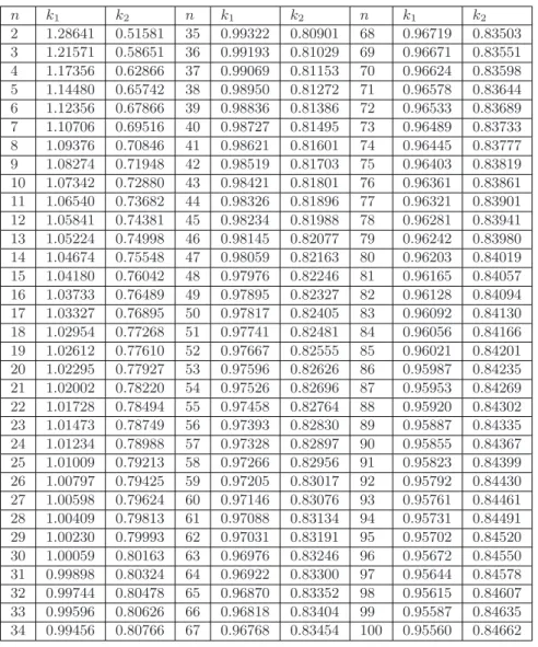
Now, the constantsk1 and k2 are required for the most common confidence
interval used in real applications, i.e., the confidence level of 95% (α = 0.05). Hence, the constants k1 and k2 for sample sizes not greater than 100 are pro-vided in Table 1.
4. The simulation study and results
Table 1: The values ofk1 and k2 for confidence level (1−α)100% =
95%
n k1 k2 n k1 k2 n k1 k2
2 1.28641 0.51581 35 0.99322 0.80901 68 0.96719 0.83503
3 1.21571 0.58651 36 0.99193 0.81029 69 0.96671 0.83551
4 1.17356 0.62866 37 0.99069 0.81153 70 0.96624 0.83598
5 1.14480 0.65742 38 0.98950 0.81272 71 0.96578 0.83644
6 1.12356 0.67866 39 0.98836 0.81386 72 0.96533 0.83689
7 1.10706 0.69516 40 0.98727 0.81495 73 0.96489 0.83733
8 1.09376 0.70846 41 0.98621 0.81601 74 0.96445 0.83777
9 1.08274 0.71948 42 0.98519 0.81703 75 0.96403 0.83819
10 1.07342 0.72880 43 0.98421 0.81801 76 0.96361 0.83861 11 1.06540 0.73682 44 0.98326 0.81896 77 0.96321 0.83901
12 1.05841 0.74381 45 0.98234 0.81988 78 0.96281 0.83941
13 1.05224 0.74998 46 0.98145 0.82077 79 0.96242 0.83980
14 1.04674 0.75548 47 0.98059 0.82163 80 0.96203 0.84019
15 1.04180 0.76042 48 0.97976 0.82246 81 0.96165 0.84057
16 1.03733 0.76489 49 0.97895 0.82327 82 0.96128 0.84094
17 1.03327 0.76895 50 0.97817 0.82405 83 0.96092 0.84130
18 1.02954 0.77268 51 0.97741 0.82481 84 0.96056 0.84166
19 1.02612 0.77610 52 0.97667 0.82555 85 0.96021 0.84201
20 1.02295 0.77927 53 0.97596 0.82626 86 0.95987 0.84235
21 1.02002 0.78220 54 0.97526 0.82696 87 0.95953 0.84269
22 1.01728 0.78494 55 0.97458 0.82764 88 0.95920 0.84302
23 1.01473 0.78749 56 0.97393 0.82830 89 0.95887 0.84335
24 1.01234 0.78988 57 0.97328 0.82897 90 0.95855 0.84367
25 1.01009 0.79213 58 0.97266 0.82956 91 0.95823 0.84399
26 1.00797 0.79425 59 0.97205 0.83017 92 0.95792 0.84430
27 1.00598 0.79624 60 0.97146 0.83076 93 0.95761 0.84461
28 1.00409 0.79813 61 0.97088 0.83134 94 0.95731 0.84491
29 1.00230 0.79993 62 0.97031 0.83191 95 0.95702 0.84520
30 1.00059 0.80163 63 0.96976 0.83246 96 0.95672 0.84550
31 0.99898 0.80324 64 0.96922 0.83300 97 0.95644 0.84578
32 0.99744 0.80478 65 0.96870 0.83352 98 0.95615 0.84607
33 0.99596 0.80626 66 0.96818 0.83404 99 0.95587 0.84635
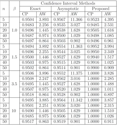
(AW) of the three confidence intervals. Twenty-four populations of Weibull distribution with shape parameter (β = 1.0, 1.5, 3.5, 10.0) and scale parameter (θ = 1.5, 2.0, 2.5, 3.0, 3.5, 4.0) were each generated of the size N = 100,000. For each population, the sample sizes of n = 5, 10, 20, 40, 50 were randomly generated 50,000 times. For each set of samples, the common 95% confidence intervals of parameter θ were constructed for the three methods. The cover-age probability (CP) and the avercover-age width (AW) are obtained by using the following two formulas:
CP = #(L≤θ≤U) 50,000 ,
AW =
P50,000
i=1 (Ui−Li)
50,000 . (33)
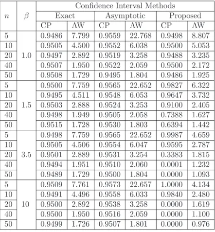
The simulation results are shown in Table 2 to Table 7. For situations of a scale parameterθ equals 1.5, 2.0, 2.5, 3.0, 3.5, 4.0, and a shape parameter β
equals 1, the results show that the coverage probabilities of the three methods close to the nominal level (0.95) and the average widths of exact and Proposed methods tend to be no difference for almost all sample sizes. In addition, the average width of Asymptotic method is wider than those of exact and Proposed methods for a small sample size (n= 5, 10), but the average widths of the three methods tend to be no difference for the larger sample sizes (n >10) for these situations. It also shows that the average widths of the three methods tend to decrease when the sample size increases for all the scale and shape parameters. For situations of a scale parameter θ equals 1.5 and a shape parameter β
equals 1.5, 3.5, 10.0 the results show that the coverage probabilities of exact and asymptotic methods close to the nominal level (0.95), whereas this of Proposed method closes to one and the average widths of exact and Proposed methods tend to be no difference for all sample sizes.
Table 2: The coverage probability (CP) and average width (AW) of 95% CIs for the scale parameter (θ) of a two parameters Weibull distribution whenθ= 1.5
n β
Confidence Interval Methods
Exact Asymptotic Proposed
CP AW CP AW CP AW
5
1.0
0.9504 3.893 0.9567 11.366 0.9523 4.395
10 0.9483 2.256 0.9535 3.027 0.9485 2.531
20 0.9496 1.445 0.9538 1.628 0.9505 1.616
40 0.9487 0.974 0.9500 1.029 0.9498 1.085
50 0.9497 0.864 0.9503 0.902 0.9496 0.961
5
1.5
0.9494 3.892 0.9554 11.363 0.9952 3.994
10 0.9496 2.255 0.9544 3.025 0.9950 2.349
20 0.9500 1.446 0.9527 1.629 0.9940 1.517
40 0.9503 0.975 0.9515 1.029 0.9916 1.025
50 0.9502 0.864 0.9514 0.901 0.9900 0.909
5
3.5
0.9506 3.896 0.9552 11.375 1.0000 3.826
10 0.9508 2.247 0.9562 3.016 1.0000 2.285
20 0.9495 1.445 0.9527 1.628 1.0000 1.488
40 0.9507 0.975 0.9520 1.029 1.0000 1.011
50 0.9518 0.864 0.9528 0.902 1.0000 0.897
5
10
0.9495 3.885 0.9564 11.342 1.0000 3.857
10 0.9501 2.251 0.9556 3.020 1.0000 2.315
20 0.9490 1.446 0.9505 1.629 1.0000 1.510
40 0.9485 0.975 0.9506 1.029 1.0000 1.026
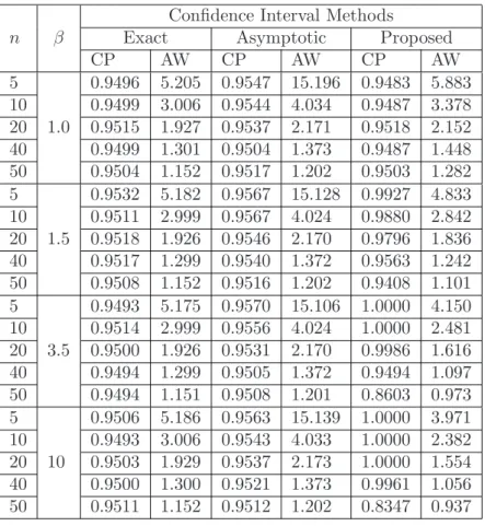
Table 3: The coverage probability (CP) and average width (AW) of 95% CIs for the scale parameter (θ) of a two parameters Weibull distribution whenθ= 2.0
n β
Confidence Interval Methods
Exact Asymptotic Proposed
CP AW CP AW CP AW
5
1.0
0.9496 5.205 0.9547 15.196 0.9483 5.883
10 0.9499 3.006 0.9544 4.034 0.9487 3.378
20 0.9515 1.927 0.9537 2.171 0.9518 2.152
40 0.9499 1.301 0.9504 1.373 0.9487 1.448
50 0.9504 1.152 0.9517 1.202 0.9503 1.282
5
1.5
0.9532 5.182 0.9567 15.128 0.9927 4.833
10 0.9511 2.999 0.9567 4.024 0.9880 2.842
20 0.9518 1.926 0.9546 2.170 0.9796 1.836
40 0.9517 1.299 0.9540 1.372 0.9563 1.242
50 0.9508 1.152 0.9516 1.202 0.9408 1.101
5
3.5
0.9493 5.175 0.9570 15.106 1.0000 4.150
10 0.9514 2.999 0.9556 4.024 1.0000 2.481
20 0.9500 1.926 0.9531 2.170 0.9986 1.616
40 0.9494 1.299 0.9505 1.372 0.9494 1.097
50 0.9494 1.151 0.9508 1.201 0.8603 0.973
5
10
0.9506 5.186 0.9563 15.139 1.0000 3.971
10 0.9493 3.006 0.9543 4.033 1.0000 2.382
20 0.9503 1.929 0.9537 2.173 1.0000 1.554
40 0.9500 1.300 0.9521 1.373 0.9961 1.056
Table 4: The coverage probability (CP) and average width (AW) of 95% CIs for the scale parameter (θ) of a two parameters Weibull distribution whenθ= 2.5
n β
Confidence Interval Methods
Exact Asymptotic Proposed
CP AW CP AW CP AW
5
1.0
0.9508 6.486 0.9569 18.936 0.9516 7.321
10 0.9499 3.754 0.9545 5.037 0.9488 4.216
20 0.9511 2.406 0.9533 2.711 0.9484 2.690
40 0.9499 1.623 0.9519 1.714 0.9497 1.807
50 0.9494 1.441 0.9504 1.504 0.9491 1.603
5
1.5
0.9491 6.468 0.9566 18.882 0.9879 5.607
10 0.9511 3.746 0.9554 5.027 0.9777 3.298
20 0.9515 2.406 0.9547 2.710 0.9514 2.130
40 0.9500 1.626 0.9513 1.717 0.8710 1.442
50 0.9516 1.440 0.9525 1.502 0.8162 1.277
5
3.5
0.9491 6.494 0.9562 18.958 0.9996 4.426
10 0.9504 3.753 0.9553 5.036 0.9962 2.646
20 0.9497 2.409 0.9522 2.714 0.8839 1.722
40 0.9490 1.626 0.9500 1.717 0.1166 1.170
50 0.9489 1.440 0.9505 1.502 0.0140 1.038
5
10
0.9493 6.478 0.9560 18.910 1.0000 4.059
10 0.9487 3.761 0.9532 5.047 1.0000 2.436
20 0.9509 2.411 0.9538 2.716 0.7439 1.590
40 0.9522 1.625 0.9523 1.716 0.0000 1.080
Table 5: The coverage probability (CP) and average width (AW) of 95% CIs for the scale parameter (θ) of a two parameters Weibull distribution whenθ= 3.0
n β
Confidence Interval Methods
Exact Asymptotic Proposed
CP AW CP AW CP AW
5
1.0
0.9486 7.799 0.9559 22.768 0.9498 8.807
10 0.9505 4.500 0.9552 6.038 0.9500 5.053
20 0.9497 2.892 0.9519 3.258 0.9488 3.235
40 0.9507 1.950 0.9522 2.059 0.9500 2.172
50 0.9508 1.729 0.9495 1.804 0.9486 1.925
5
1.5
0.9500 7.759 0.9565 22.652 0.9827 6.322
10 0.9495 4.511 0.9548 6.053 0.9647 3.732
20 0.9503 2.888 0.9524 3.253 0.9100 2.405
40 0.9498 1.949 0.9505 2.058 0.7388 1.627
50 0.9515 1.728 0.9530 1.803 0.6394 1.442
5
3.5
0.9498 7.759 0.9565 22.652 0.9987 4.659
10 0.9505 4.506 0.9554 6.047 0.9595 2.787
20 0.9501 2.889 0.9531 3.254 0.3383 1.815
40 0.9494 1.951 0.9510 2.060 0.0001 1.232
50 0.9489 1.729 0.9500 1.804 0.0000 1.093
5
10
0.9509 7.761 0.9573 22.657 1.0000 4.134
10 0.9491 4.496 0.9558 6.033 0.9840 2.480
20 0.9500 2.892 0.9538 3.258 0.0000 1.619
40 0.9500 1.950 0.9516 2.059 0.0000 1.100
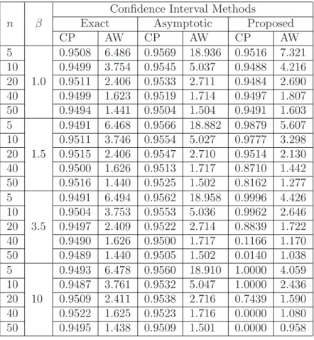
Table 6: The coverage probability (CP) and average width (AW) of 95% CIs for the scale parameter (θ) of a two parameters Weibull distribution whenθ= 3.5
n β
Confidence Interval Methods
Exact Asymptotic Proposed
CP AW CP AW CP AW
5
1.0
0.9522 9.061 0.9579 26.453 0.9522 10.220
10 0.9521 5.257 0.9552 7.054 0.9498 5.912
20 0.9492 3.373 0.9523 3.800 0.9501 3.769
40 0.9510 2.271 0.9530 2.397 0.9499 2.528
50 0.9489 2.016 0.9500 2.103 0.9481 2.243
5
1.5
0.9505 9.094 0.9564 26.549 0.9793 7.036
10 0.9515 5.260 0.9566 7.058 0.9514 4.136
20 0.9508 3.374 0.9527 3.801 0.8564 2.668
40 0.9495 2.275 0.9519 2.401 0.5896 1.803
50 0.9487 2.016 0.9500 2.104 0.4560 1.599
5
3.5
0.9516 9.079 0.9572 26.506 0.9946 4.872
10 0.9498 5.251 0.9555 7.046 0.8107 2.912
20 0.9492 3.373 0.9512 3.799 0.0252 1.896
40 0.9506 2.276 0.9517 2.403 0.0000 1.288
50 0.9519 2.015 0.9531 2.102 0.0000 1.142
5
10
0.9497 9.110 0.9553 26.597 1.0000 4.202
10 0.9499 5.246 0.9546 7.040 0.1284 2.519
20 0.9508 3.379 0.9537 3.806 0.0000 1.644
40 0.9502 2.275 0.9520 2.402 0.0000 1.117
Table 7: The coverage probability (CP) and average width (AW) of 95% CIs for the scale parameter (θ) of a two parameters Weibull distribution whenθ= 4.0
n β
Confidence Interval Methods
Exact Asymptotic Proposed
CP AW CP AW CP AW
5
1.0
0.9498 10.363 0.9564 30.254 0.9498 11.708
10 0.9507 5.997 0.9562 8.047 0.9511 6.737
20 0.9502 3.850 0.9536 4.337 0.9493 4.302
40 0.9499 2.599 0.9516 2.744 0.9498 2.897
50 0.9502 2.301 0.9517 2.401 0.9492 2.561
5
1.5
0.9498 10.381 0.9549 30.306 0.9723 7.691
10 0.9503 6.008 0.9548 8.061 0.9314 4.513
20 0.9496 3.856 0.9526 4.344 0.7925 2.916
40 0.9501 2.600 0.9517 2.744 0.4472 1.970
50 0.9497 2.305 0.9513 2.405 0.3007 1.748
5
3.5
0.9492 10.381 0.9554 30.307 0.9812 5.062
10 0.9496 6.016 0.9542 8.073 0.5227 3.026
20 0.9493 3.853 0.9527 4.341 0.0001 1.971
40 0.9510 2.598 0.9523 2.743 0.0000 1.337
50 0.9497 2.303 0.9505 2.403 0.0000 1.187
5
10
0.9511 10.361 0.9573 30.248 0.9984 4.255
10 0.9507 5.990 0.9555 8.038 0.0000 2.553
20 0.9510 3.859 0.9537 4.347 0.0000 1.666
40 0.9497 2.599 0.9508 2.744 0.0000 1.132
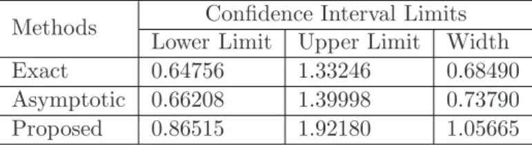
Table 8: The 95% CIs for the scale parameter (θ) of a Two Param-eters Weibull Distribution for Urinary Tract Infection (UTIs) Data
Methods Confidence Interval Limits Lower Limit Upper Limit Width
Exact 0.64756 1.33246 0.68490
Asymptotic 0.66208 1.39998 0.73790
Proposed 0.86515 1.92180 1.05665
5. Real example: Urinary Tract Infection Data
In this section, a real-life example is given for the data from a healthcare depart-ment to illustrate the application of the three methods of confidence intervals. The data are collected from a large hospital to monitor urinary tract infections (UTIs). The data represent the number of days in between the admission and discharge of male patients. The frequency of patients having discharged from hospital on being acquired the UTIs while in the hospital is mentioned to quickly identify an increased infection rate. The similar data of UTIs were used by [27], [28] and [29]. According to [29] the data follow a Weibull distribution with shape parameter β = 2. The summary statistics for the data are given as fol-lows: n= 30,Pn=30
i=1 X β
i = 26.9702, X ∗
= 0.961129, k1 = 1.00059, k2 = 0.80163.
The resulting 95% confidence intervals for the three confidence interval methods and the corresponding confidence widths are given below in Table 8.
From Table 8, it is found that all the three methods for the 95% confidence intervals of the scale parameter (θ) have the lower and upper limits between 0.64756 to 1.92180, that is, the scale parameter (θ) of a two parameters Weibull distribution for urinary tract infections (UTIs) data seems to be not greater than two with a shape parameter β = 2. In addition, exact method has the shortest interval width. This conforms to the simulation study that the exact confidence interval performs well efficiency when it compares to the asymptotic and Proposed confidence intervals for the case of a small scale parameter and shape parameterβ = 2.
6. Concluding remarks
one sample problem using the pivotal-based approach are derived. A Monte Carlo simulation study is performed to compare the efficiencies in terms of two criteriathe coverage probabilities and average widths of confidence intervalsfor the exact, asymptotic and approximate confidence intervals. It is found that the coverage probabilities of the three confidence intervals are close to the nom-inal level in cases of the shape parameterβ equals 1 and all scale parametersθ
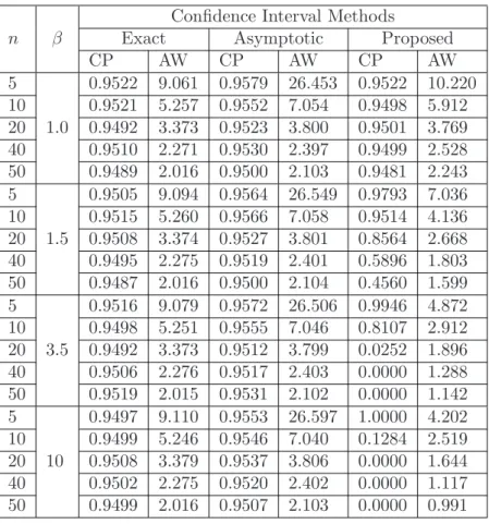
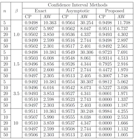
for all sample sizes. When a shape parameter β increases, the coverage prob-abilities of the exact and asymptotic confidence intervals are also close to the nominal level for all sample sizes, whereas the coverage probability of the ap-proximate confidence interval closes to one for a small sample size and it tends to decrease when a sample size increases. When considering the efficiency in term of the average width, it is found that the average widths of the three confidence intervals tend to be no difference in cases of the shape parameter
β equals 1 and all scale parameters θ for the large sample sizes. Moreover, in case of the shape parameter β is greater than 1 (β = 1.5, 3.5, 10.0) and the scale parametersθis greater than 1.5 (θ= 2.0,2.5,3.0,3.5,4.0), the approximate confidence interval tends to have the shortest average width for all sample sizes. However, asymptotic confidence interval tends to perform poor efficiency for a small sample size whatever the shape and scale parameters will be. Finally, the approximate confidence interval is easy to compute and it tends to have the coverage probability close to one and have the shortest average width for a small sample size (n = 5) and almost all the shape and scale parameters, therefore it can be recommended for the practitioners in these cases.
References
[1] W. Weibull, A statistical distribution function of wide applicability,ASME Journal of Applied Mechanics,18(1951), 293–297.
[2] N.L. Johnson, S. Kotz, Continuous Univariate Distributions – I, Wiley, New York (1970).
[3] B. Dodson,Weibull Analysis, ASQC Press, Wisconsin (1994).
[4] W. Nelson,Applied Life Data Analysis, Wiley, New York (1982).
[5] W.Q. Meeker, L.A. Escobar,Statistical Methods for Reliability Data, Wiley, New York (1998).
[7] B. Dodson,The Weibull Analysis Handbook, 2nd Ed., ASQ Quality Press, Milwaukee (2006).
[8] J. Neyman, Outline of a theory of statistical estimation based on the clas-sical theory of probability,Philosophical Transactions of the Royal Society Series A,236(1937), 333–380.
[9] R.V. Hogg, E.A. Tanis,Probability and Statistical Inference, 6thEd.,
Pren-tice Hall, New Jersey (2001).
[10] G. Casella, R.L. BergerStatistical Inference, 2ndEd., CA Duxbury, Pacific
Grove (2002).
[11] N. Balakrishnan, E. Cramer, G. Iliopoulos, On the method of pivoting the CDF for exact confidence intervals with illustration for exponential mean under life-test with time constraints,Statistics and Probability Letters, 89
(2014), 124–130.
[12] J. Sinsomboonthong, Confidence interval estimations of the parameter for one parameter exponential distribution, IAENG Internat. J. of Applied Mathematics,45, No 4 (2015), 343–353.
[13] Y. Cho, H. Sun, K. Lee, Exact likelihood inference for an exponential pa-rameter under generalized progressive hybrid censoring scheme,Statistical Methodology,23(2015), 18–34.
[14] M.O.A. Abu-Shawiesh, H.E. Aky¨uz, B.M.G. Kibria, Performance of some confidence intervals for estimating the population coefficient of variation under both symmetric and skewed distributions, Statistics, Optimization and Information Computing: An Internat. J.,7, No 2 (2019), 277–290. [15] A.M. Mood, F.A. Graybill, D.C. Boes,Introduction to the Theory of
Statis-tics, 3rd Ed., McGrawHill, Singapore (1974).
[16] N. Mukhopadhyay, Probability and Statistical Inference, Marcel Dekker Inc, New York (2000).
[17] M.O.A. Abu-Shawiesh, Adjusted confidence interval for the population median of the exponential distribution, J. of Modern Applied Statistical Methods,9, No 2 (2010), 461–469.
[19] L. Zhang, M. Xie, L. Tang, A study of two estimation approaches for parameters of Weibull distribution based on WPP.Reliability Engineering
&System Safety,92(2007), 360–368.
[20] N. Balakrishnan, M. Kateri, On the maximum likelihood estimation of parameters of Weibull distribution based on complete and censored data,
Statistics and Probability Letters, 78(2008), 2971–2975.
[21] A.O.M. Ahmed, H.S. Al-Kutubi, N.A. Ibrahim, Comparison of the Bayesian and maximum likelihood estimation for Weibull Distribution, J. of Mathematics and Statistics,6, No 2 (2010), 100–104.
[22] L. Barker, A comparison of nine confidence intervals for a Poisson parame-ter when the expected number of events is≤5,The American Statistician,
56, No 2 (2002), 85–89.
[23] M.B. Swift, Comparison of confidence intervals for a Poisson meanFurther considerations,Communications in StatisticsTheory and Methods, 38, No 5 (2009), 748–759.
[24] V.V. Patil, H.V. Kulkarni, Comparison of confidence intervals for the Pois-son mean,REVSTAT–Statistical J.,10, No 2 (2012), 211–227.
[25] L.J. Bain, M. Engelhardt, Introduction to Probability and Mathematical Statistics, 2nd Ed., Duxbury Press, Belmont, CA (1992).
[26] L.S. Nelson, A control chart for parts-per-million nonconforming items, J. of Quality Technology, 26(1994), 239–240.
[27] E. Santiago, J. Smith, Control charts based on the exponential distribution: Adapting runs rules for the t chart,Quality Engineering,25, No 2 (2013), 85–96.
[28] M. Aslam, N. Khan, M. Azam, C.H. Jun, Designing of a new monitoring t-chart using repetitive sampling,Information Sciences,269 (2014), 210– 216.