HYPERION
INTERNATIONAL
JOURNAL
Hyperion International Journal of Econophysics & New Economy
Volume 1, Issue 1, 2008
ECONOPHYSICS Section
Ion Spânulescu and Anca Gheorghiu, An econophysics model for investments and economic development... 7
Irina Dmitrieva, Diagonalization problems in classical Maxwell theory and their industrial applications ... 23
Gheorghe Săvoiu, Statistical thinking and statistical physics... 37
Wolfgang Ecker-Lala, Description and analysis of fuzzy information ... 51
Cristina Burghelea, The neuromarketing – an instrument of the traditional marke-ting techniques ... 61
NEW ECONOMY Section
Cristina Raluca Popescu, Scientific knowledge in the complexity of the new economy ... 77
Elena Pelinescu, Andrei Silviu Dospinescu and Petre Caraiani, The role of expected and perceived inflation in the dynamic of inflation implications on the cost of living ... 95
Ana Maria Grigore, The importance of human resources in the new economy ... 109
Andrei Cristea and Tiberiu Diaconescu, Risk management in economics – firm performance ... 119
Veronica Adriana Popescu, Knowledge, a strategic asset able to encourage Romania’s competitiveness... 139
AN ECONOPHYSICS MODEL
FOR INVESTMENTS
AND ECONOMIC DEVELOPMENT
Ion SPÂNULESCU* and Anca GHEORGHIU**
Abstract. Most of the econometric and econophysics models have been
borrowed from the statistical physics, and as a consequence, a new interdis-ciplinary science called econophysics has emerged. In this paper we planned to extend the analogy between different economic processes or phenomena and processes/phenomen from different fields of physics, other than statistical physics. On the basis of the economic development process and amplification phenomenon analogy, a new econophysics model, named “economic amplifier”, on the electronic amplification principle from applied physics was proposed and largely analyzed.
Keywords: econophysics models, electronic amplifier, β economic
amplifica-tion coefficient.
1. Introduction
Economic phenomena, processes and complex structures analyses imply theories and models borrowed from some other sciences, especially from exact sciences (mathematics) or/and nature sciences (physics) where laws and phenomena have an exact character, a determinist one. Such approches guiding to interdisciplinary directions of studies and analyse allowing quantitative determinations and forecasting for economic scien-ces, are met in econometry and econophysics.
As known, the economic forecast projective models, for modelling of various economic activities etc., are widely and successfully applied in economic theory and practice. The confirmation of the validity of these widely used models is of paramount importance and great theoretical and practical interest. If this confirmation comes from the exact sciences and from the natural laws’ sciences (physics and chemistry) has endorsed a high accuracy, due to the use of the exact sciences, being checked by the
physical laws in accordance with the laws of nature. And this is the great importance of econophysics for economic theory and practice.
If the physics or econophysics models confirm various economic models, established by economic science or practice (the Keynes, Domar, Cobb-Douglas models etc.), then they get the endorsement of accuracy and that of well founded theoretical laws or equations existing not only as semi-empirical equations but as well defined economic laws.
Physics, is the most suitable for modeling the economic phenomena and structures or financial-banking operations, because it takes into consideration the process variables characteristics and permits to use some procedures – including the mathematical one – especially probability theory for minimizing or eliminating such influences depending on human factor.
During last decade, on the basis of many studies and published papers and books, a new interdisciplinary science has appeared named econo-physics, which uses models taken especially from statistical physics to describe some economic phenomena and processes.
Most econophysics approaches, models and papers that have been written so far refer to the economic processes including systems with a large number of elements (such as financial or banking markets, stock markets, incomes, production or product’s sales, individual incomes etc.) where statistical physics methods, and Boltzmann, Gibbs and some other statistical distribution types are mainly applied [1÷16].
Reducing econophysics only to of statistical physics applications in economy, especially in the stock-markets analysis, seems to be very res-trictive. It is desirable to investigate other fields of physics, and economy too, in which processes similarity inspire and even facilitate to adopt new econophysics models using – where it is possible – some other physics fields too.
This paper proposes an extension of analogy between different econo-mic phenomena and processes and phenomena or processes from different fields of physics, other than statistical physics, especially from electronic physics and condensed matter (solid state) physics.
2. Economic growth and development represents
an amplification phenomenon
obtain benefits i.e. profit or an increase in initial investment. In other words, growth or economic development is an amplification phenomenon similar to the phenomenon of amplification of physics and engineering which is produced by devices as transistors or amplification integrated circuits. So the economic growth means the amplification of the value of utilised and processed resources. In this way, taking in conside- ration the importance of economic development model and production amplification, in this paper a model based on amplification concept from electronic physics, named economic amplifier was proposed and discussed. The model implies an electronic amplifier realized with active electronic devices, the most by used being the device named transistor, which represents itself an excellent amplifier, of both current and electrical power [17,18].
The transistor and the electronic amplifier made of transistors, present the features of an exact model, a determinist one. Thus, if the transistor is used for economic modeling, it guarantees the same accuracy and validity to the economic models to which the electronic amplifier model is corre-lated and assimicorre-lated.
This is the reason why in the next section the principles of the elec-tronic amplifier will be briefly presented.
3. Electronic Amplifier
Any electronic amplifier has an active element which is either bipolar transistor (with p-n junctions) or field effect transistor (MOS type).
In this section we are going to present some parameters and charac-teristics of bipolar transistor with p-n junctions and the MOSFET structure and characteristics.
3.1. The bipolar transistors
As it can see in figure 1,a, the bipolar transistor is made of two semiconductor p-n junctions, first junction (emitter junction) being forward biased with positive voltage, and the second one (collector junction) being reverse biased with voltage, with:
BE
V
CB
V
(1) .
| | |
By proper biasing of the junctions, the transistor will be crossed by emitter, base and collector currents and which are in the following [17,18]:
B E I
I ,
( IC)
C B E I I
I = + (2)
in which represent the current due to injection of charge carriers from emitter region to base region where they are transferred into collector circuit as collector current under the action of electric field of collector junction (Fig. 1,a).
E
I
C
I
- + - +
IE IC
IB
VBE VCB
B p
( )
C n
( )
E n
( )
a) b) Figure 1. a) The structure and bias for the n-p-n bipolar transistor;
b) the symbol for the n-p-n bipolar transistor.
Due to inverse currents of minority carriers from collector and emitter regions and recombination current of charge carriers in the base region, the base current IB is much smaller than IE or IC :
IB << IC (3)
.
E C I
I ≈
a) b)
Figure 2. a) The n-p-n transistor common emither (CE) configuration;
b) Simplified representation of an electronic amplifier.
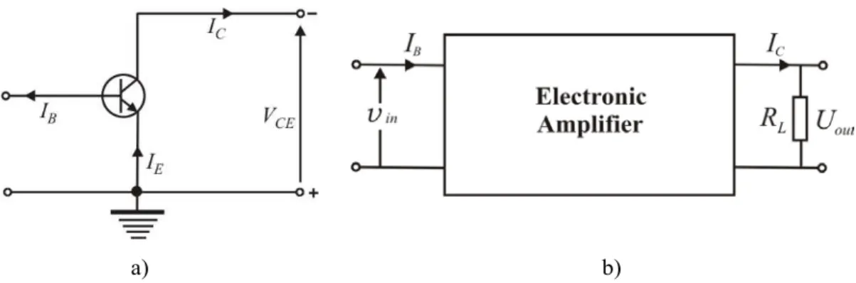
A simplified representation of the electronic amplifier with the bipolar transistor in common emitter configuration is given in figure 2,b.
The current amplification coefficient for transistor in CE confi-guration represent the ratio between output current that is collector current and input current that is
,
out
I
,
C
I Iin IB :
. B C in out I I I I = =
β (4)
Replacing IB from equation 2 in relation 4 we obtain:
. 1 > > − = = β C E C B C I I I I I (5)
because From (5) it can be noticed that the bipolar transistor in CE configuration is a very good current amplifier because amplification coefficient β is much grater than 1 (usually β = 100 ÷1000 or more).
. ~ E C I
I <
Generally, the transistor, like any other amplifier, is used to amplify variable signals, υin, all these being much smaller then biasing voltages:
. |
|vin <<VBE (6)
In this case we have the dynamic regime of transistor functioning to small signals, when voltages and/or variable currents can be considered as little variations of the biasing currents or voltages [18]:
C C BE BE
in =V = ΔV ; i = ΔI
v etc.
3.2. Unipolar Metal-Oxide-Semiconductor (MOS) transistors
The unipolar transistors also contain two p-n junctions but they are functioning with only one charge carriers type, the majority ones (where their name came from) on the basis of field effect, being named Field Effect Transistors (FET) also [17,18].
There are several types of these transistors but the most often used in current applications is Metal-Oxide-Semiconductor (MOS) transistor where control electrode named Gate is isolated from the device through an oxide or dielectric thin film (Fig. 3,a).
The analog of emitter from bipolar transistor is the Source (S) where charge carriers are coming from, and the analog of collector is the Drain (D) that is collecting the carriers (Fig. 3,a,b).
Silicon dioxide film
hole
electron
n-type channel
Source Gate Drain
•
Substrate
a) b)
Figure 3. a) FET structure of n channel-MOS type;
b) The conduction channel induced in the MOSFET structure.
Initially, the source and drain regions are completely isolated so there is no current flowing in the MOS structure from figure 3,a, between source and drain. If a positive voltage is applied between gate and source there will appear a conduction channel of n-type between source and drain where the electrons there the majority carriers will be able to flow (Fig. 3,b).
The channel that has been formed is one that has been induced due to gate positive potential action that will reject the holes from the region placed exactly under oxide to semiconductor depth of p-type substrate. The positive gate voltage will attract the mobile electrons from the
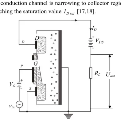
After channel creation between drain and source, if a positive voltage is applied, the electrons injected into the source (by biase voltage) will flow to drain through channel, and therefore, a drain current will result (Fig. 4). By varying input voltage (which includes a variable voltage that must by amplified), the thickness and electrical resistance of induced n-channel will vary (Fig. 4) and, as a consequence, the drain current will vary, too. In this way, an amplified output voltage Uout can
be taken from load resistor RL: 0
>
DS
V
D
I
GS
V
in
v
D
I
Uout = IDRL. (8)
From figure 4 it can be seen that as result of applying voltage the n-conduction channel is narrowing to collector region limiting current reaching the saturation value [17,18].
, 0 >
DS
V
D
I IDsat
ID
D V
DS
G
RL Uout
VG
vin
Figure 4. MOSFET in the amplification regime (ID≠0).
For the MOS transistor the slope S or transconductance gm is defined
as [18]:
.
P D m
V I S g
∂ ∂ =
= (9)
PMOSFET (p-MOS Field Effect Transistor) with p-type induced channel is functioning in the same way where source and drain regions of
those of NMOSFET, so VPS <0 and VDS <0. In both cases, MOS
transistors are functioning with only one type of charge carriers: electrons or holes, so they are unipolar transistors.
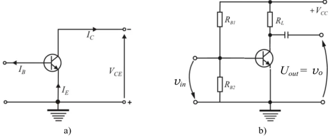
3.3. Electronic amplifier with bipolar transistors
Figure 5,b represents a practical circuit of an amplifier with bipolar transistor in common emitter (CE) configuration (Fig. 5,a and Fig. 2,a). To avoid using a supplementary source for VBE voltage, a voltage divider
for proper biasing of base (input circuit) in used. The amplifier has only one amplification stage because it uses only one transistor (active element) for amplification. To increase the amplification, the amplifiers with two or more transistors, having two or more amplification stages are used [17].
, 1
B
R RB2
Uout = vo
vin
a) b)
Figure 5. a) The n-p-n transistor common emitter (CE) configuration;
b) amplifier circuit with a bipolar transistor in CE configuration.
If a small variable signal vin is applied to amplifier input (Fig. 5,b) an
amplified signal is taken from load resistor as output voltage (see also Fig. 2,b):
L
R
.
out L
c
o =i R =U
v (10)
The current amplification coefficient is given by Eq. (4) that is practi-cally the same with current amplification coefficient for the variable signals:
.
b c
i i
=
Also, an amplified power is put out on the load resistor RL (Fig. 2,b):
(12) 2
c L c L c c out
out U i i R i R i
P = = =
these obtaining a power gain of the signal applied to amplifier input.
4. Economic Amplifier
In this paper a model based on transistor-effect from physics, meaning amplification phenomenon that can be realized using transistors, was proposed. Such a model can be used for modeling different economic structures or processes such as production or investment fields, steady capital, founds or financial – banking fields, stocks etc.
Transistor-effect of amplification of transistor device is completely verified in practical activities. Modeling physical phenomena on the elec-tronic level for bipolar and unipolar transistors theory is validated through all technological and socio-economical developments of nowadays society, this little device being the base brick of all electronic apparatus and equipments in any field of activity. The same overwhelming confirmation of transistor model validity (which is multiplied in hundreds and thousand millions of components into microprocessors or some other integrated systems) gives to the transistor the leader status of all contemporary dis-coveris and practical applications in physics and techniques. That’s why the transistor deserves the whole attention of researchers that are studying models of different human activity phenomena and processes, especially economics, finances, management etc. The almost universal validity of amplification phenomenon, in particular by transistor-effect, guarantees the validity of economic model action on the basis of electronic amplifier with transistors, that we named “economic amplifier model”.
First example of similitude and modeling with transistor model is represented by assimilation of charge carriers in transistors with the number of products realized inside a production section or a factory etc. by an economic unit.
As charge carriers current flows through transistor from input to output (Fig. 1), the products flow from input (where they represent parts, raw materials etc.) to the output of a section production or a manufacture and then all this stuff is delivered as finite products.
The role of load resistor from output circuit (Fig. 2,b) is taken by storage or transportation (conveyors, containers, trains etc.) systems which
L
deliver products to consumers in the same way in which charge carriers are collected from load resistor as current intensity IC.
The expression represents the output voltage being assimilated with technical platform – production ensemble from workshop, manufac-ture or factory etc. where equipments, labour force (human factor) and other production expenses are included.
L CR
I
The charges carried by charge carriers are assimilated with values that final products are carrying that represent “valor carriers”.
The economic amplifier can be interpreted as an Input-Output model like one stage transistor electronic amplifier. So, economic amplifier model can be analyzed using Eq. (8) for current amplification coefficient, β, of bipolar transistor: . in out I I =
β (4')
In this way if we consider that at the input circuit, between base and emitter a signal assimilated with investments (capital or in nature) introduced into factory (economic unit) is applied and at the output as current we consider the total amount of products or total income obtained, we can define so called βeconomic coefficient. This coefficient can be defined for all quantity of products
out
I
p
β as:
equipments and finite materials raw products of quantity Total economic s, Investment =
βp . (13)
A more important parameter can be introduced being the ratio of the value efficiency determined by the total amount of incomes (business value) shared over the investment amount, marked by βv:
Expences s Investment Incomes Total + =
βv economic . (14)
physics (electronics). Otherwise, the gain obtained from banks, stocks etc. is similar to the gain obtained from transistor amplifiers where we have a gain for bank (equivalent with the gain for current, β given by Eq. (4)):
input
at theAmount obtained Given Interests) capital
(initial Values
Total
output at the obtained etc.)
interests (money,
Values
+ +
=
βbank . (15)
Obviously, the amplification factor βbank is calculated for a period of
standard time (for example: a year, a month, a week etc.) that is, over the time, of the financial operations execution.
The bankruptcy of an economic agent (company, banks etc.) is modeling by the transistor breakdown or circuit failure. Circuit damage analysis could inspire solutions for bankruptcy avoidance. Transistor bur-ning (bipolar or unipolar) could come from exploitation errors (improper voltages), supercharges, design errors, or because of semiconductors material quality, that is, for the reasons associated to the improper structure and design of the material, device (transistor) or circuit (amplifier). Similar these types of errors are also met because the managerial drawbacks, lower staff qualification, lack of communication, improper average age for a specific production stage of the company etc.
The modeling using more transistors and more amplifying stages can be used for the bigger economic systems such as big factories or corpo-rations etc. So, one stage amplifier (using one transistor) is modeling one section activity. The multi-stage amplifiers having a big gain can simulate a factory with many sections. The bigger amplifier with many stages includ-ing the output power one are used to model a corporation or a big trust having a very large gain (amplification coefficient) and manufacturing a large amount of products [17].
5. Economic development modeling using
the economic amplifier model
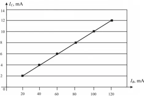
The economic amplifier model can be very well applied for modeling the economic development based on the initial investments both at the micro and the macroeconomic levels [19]. So, for the bipolar transistor (CE configuration), the output current IC (mA) as a function of
input current, IB (μA), therefore, β, given by Eq. (4), has a linear
IC, mA
IB, mA
Figure 6. IC = f(IB) dependence represents a straight line.
Indeed, the Eq. (4) can be written as:
B
C I
I =β (16)
representing a straight line (when β = const) intersecting the origin of the axes. If it is not the case and the intersection with vertical axis is a0, Eq. (16) is becaming:
B
C a I
I = 0+β (17)
also representing a straight line.
The Eq. (16) is a simple regression one, exactly as the equation obtained for the one-variable (“one-factorial”) econometric model [19,20] for which a0, and β are the regression coefficients. Therefore the economic
amplifier model is a true econometric model and implicitly an econo-physics one.
Under normal conditions and economic policies by applying the economic amplifier model for the investments, one may see that the total incomes as a function of inputs (investments, materials etc.) are also a linear or near linear function (Fig. 7 and Fig. 8) justifying the econophysics model we have proposed.
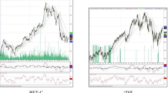
The economic amplifier model can be also very well applied on the macroeconomic level. A good example is given in figure 8 where the dependence of the Gross Domestic Product (G.D.P.) of Romania as a function of the capital accumulation between 1990-2005 years is repre-sented. As it can be seen from figure 8, the resulting function has a near linear dependence. The medium value of 5.19 for the economic β at national level is calculed.
Figure 7. Incomes representation depending
of expenses for a small manufacture.
Figure 8. Gross Domestic Product of Romania vs. Gross Capital Formation
Apart from the normal development for which Incomes = f (Invest-ments) dependence is a line or a monotonous rising curve, there are situations in which after a monotonous rising, the descending slopes appears signaling the appearance of the disturbing elements generated in special by human factor, damaging economic policies, crises, inefficient management or even political influences (totalitarian states). In such cases, when investments and equipment lifetime (T) had not been consumed, but the dependence isn’t a line or a monotonous rising curve, the parameters on the basis of the investment must be reconsidered and any negative influences, restrictive policies etc. must be eliminated, in order to put the business on the normal trend of rising.
Such considerations may seem (appear) obvious or of good sense, but it is important to remind that all these are in concordance with economic amplifier model which we have proposed here.
6. Conclusions
A new econophysic model, on the basis of the amplification phenomenon from applied physics, that can be realized using transistors, integrated circuits or other electronic active devices, was proposed and analyzed.
This new model, named economic amplifier, can be used for mode-ling different economic structures or processes such as production or investment fields, steady capital, founds or financial-banking fields, stocks etc.
The accuracy of electronic transistor and of electronic amplifier functioning, confirmed through all nowadays supertechnology, can confer a solid guaranty for the economic amplifier model also in the economic fields where such model is applied.
As it shown in previosly papers [19,20], the economic amplifier model can explain and confirms the justness and validity of other econometric models from the investments field.
REFERENCES
11. D. K. Faley, A Statistical Equilibrium Theory of Markets, J. Econ. Theory, 62
321-345 (1994).
12. R. N. Mantegna and H. E. Stanley, An Introduction to Econophysics, Cambridge University Press, Cambridge, 2000.
13. A. A. Drăgulescu and V. M. Yakovenko, Statistical Mechanics of Money, Eur. Phys. J. B. 17, 723-729 (2000).
14. A. A. Drăgulescu and V. M. Yakovenko, Evidence for the Exponential Distribu-tion of Income in the USA, Eur. Phys. J. B. 20, 585-589 (2001).
5. I. Antoniou, P. Akritas, D. A. Burak, V. V. Ivanov, A.V. Kryanev and G. V. Lukin, Robust Methods for Stock Market Data Analysis, Physica A: Statistical Mechanics and its Applications 336 (3-4), 538-548 (2004).1
6. R. N. Mantegna, Z. Palagyl, H. E. Stanley, Applications of Statistical Mechanics to Finance, Physica A 274, 216 (1999).
7. F. Lillo and R. N. Mantegna, Variety and Volatility in Financial Markets, Phys. Rev. E. 62, 6126-6134 (2000).
8. V. M. Eguiluz, M. G. Zimmernann, Transmission of Information and Herd Behavior: An Application to Financial Markets, in Physical Review Letters, 85,
5659-5662 (2000).
19. A. A. Drăgulescu, V. M. Yakovenko, Probability Distribution of Return in the Heston Model with Stochastic Volatility, Quantitative Finance, vol. 2, 443-453 (2002).
10. V. Plerou, P. Gopikrishman, L. A. N. Amaral, M. Meyer and H. E. Stanley, Sca-ling of the Distribution of Financial Market Indices, Phys. Rev. E 60, 5305-5316
(1999).
11. Terence C. Mills, Statistical Analysis of Daily Gold Price Data, Physica A: Statistical Mechanics and its Applications 338 (3-4), 559-566 (2004).
12. Hajime Inaoka, Hideki Takayasu, Tokiko Shimizu, Takuto Ninomiya and Ken Taniguchi, Self-Similarity of Banking Network, Physica A: Statistical Mechanics and its Applications 339 (3-4), 621-634 (2004).
13. Araceli Bernabe, Esteban Martina, Jose Alvarez-Ramirez and Carlos Ibarra-Valdez, A Multi-model Approach for Describing Crude Oil Price Dynamics, Physica A: Statistical Mechanics and its Applications 338 (3-4), 567-584 (2004).
14. Tomoya Suzuki, Tohru Ikeguchi and Masuo Suzuki, A model of complex behavior of interbank exchange markets, Physica A: Statistical Mechanics and its Appli-cations 337 (1-2), 196-218 (2004).
15. H. Levy, M. Levy and S. Solomon, Microscopic Simulation of Financial Markets, Academic Press, San Diego, 2000.
16. M. Gligor, Margareta Ignat, Econophysics (in Romanian), Economic Publishing House, Bucharest, 2003.
17. I. Spânulescu (Edit.), Electronics (in Romanian), Didactic and Pedagogic Publi-shing House, Bucharest, 1983.
19. Anca Gheorghiu, Ion Spanulescu, New Approaches and Econophysics Models (in Romanian), Victor Publishing House, Bucharest, 2004.
DIAGONALIZATION PROBLEMS
IN CLASSICAL MAXWELL THEORY
AND THEIR INDUSTRIAL APPLICATIONS
Irina DMITRIEVA*
Abstract. Present results concern the diagonalization problem of the
arbitrary n-dimensional operator equations system over the arbitrary m-dimensional space. The known elements are the arbitrary operators that act in certain class. The only requirement of the proposed diagonalization method is the operators’ commutativity in pairs. The proposed algorithm is invariant to the matrix structure of the initial system which may have the arbitrary block construction, and the diagonalizing procedure acts in the consecutive order beginning from the external till the last inner matrix block elements.Moreover, the given method doesn’t depend on the initial and boundary conditions which become necessary only when the diagonalizing process is finished completely. Additionally, this algorithm deals only with the operators that form the matrix of the original system. Hence, these operators explicit expressions are known in advance and the described diagonalizing procedure “knows” beforehand what kind of operator and when it is applied.The proposed method and calculus, though are absolutely correct mathematically, are rather simple in their direct application and do not require from the engineer or some other non-expert the knowledge of the generalized function theory that is used almost in all diagonalization applied problems even for the usual linear PDEs systems.Thus, the present results in their specific case of the PDEs operator system over the classical Maxwell space were applied to the solution of concrete engineering problems that concerned the signal transmission in various media.
Keywords: diagonalization, system of the PDEs operator equations, vector
function, scalar equation, Maxwell space.
1. Introduction
It is well known that the majority of real physical processes may be described by the PDEs or by their systems. That’s why even now the problem of simply applied and mathematically correct algorithm for the
* Math. Analysis Dept., Institute of Physics and Mathematics, SouthUkr. State PedUniv.,
various classes of the PDEs systems’ explicit solution remains quite urgent not only in the current physics and engineering, but in the applied mathematics as well [1]-[3]. The classical approach here is the method of integral transformations jointly with the generalized functions theory [2].
In the case of the first studied direction the original PDEs system after application of the corresponding integral transformation is reduced to the ODEs or algebraic equations system in terms of the initial functions’ transformants. But when the applied problem is studied by means of the above mentioned method one must be very cautious in choosing the correct integral transformation. In other words, the integral transformation has to be chosen correctly not only mathematically but also considering physical or engineering features of the initial statement.
Turning towards the generalized functions method it should be noted that this approach, though is very elegant mathematically, remains rather difficult for the non mathematicians at the stage of its explicit realization. Thus, for example, in monograph [2, p. 127-201], even in the simple systems’ case of the differential operator polynomials with constant coefficients from the very beginning the researcher has to deal with integral transformations which operate in various classes of the generalized functions, just as: basic, moderate and quickly increased. Hence, when an engineer or some other non expert even at the stage of system diagonal-lization procedure uses the both of the above mentioned methods, he must be very acute in all their mathematical details. Moreover, for each specific class of systems these approaches are realized in their own way [2].
With the problem of the PDEs first order systems’ solution over the space ( , , , )x y z t the author has come across investigating the classical electrodynamics objects and Maxwell equations in particular [4]. Thus, in [5] was considered the case of linear homogeneous isotropic undisturbed media with the outside currents, and only two main postulates of classical electrodynamics as the following vector equations were accepted:
⎧ ⎨ ⎩
0
0
CT a
a
rotH E E j
rotE H
σ ε μ
= + ∂ +
− = ∂
r r r r
r r (1)
In (1): Er =E x y z tr( , , , ) and Hr =H x y z tr( , , , ) are the unknown vector functions of the electric and magnetic field tension; differential operator
0
t
∂ ∂ =
∂ ; the given vector function ( , ,
CT CT , )
j = j x y z t
r r
, a, a
describes the outside
absolute permeance and dielectric permeability correspondingly. In [5] this vector system (1) was reduced to the equivalent system of six PDEs, and each equation held only one unknown scalar vector component
or . In other words, the original matrix system was diagonal-lized. Such result was obtained by the consistent application of the corresponding differential operators to six original equations of (1) that were written in terms of
{ }
{ }
3 1 i iEr = E =
{ }
3 1 i iHr = H =
3 1 i i
E = and
{ }
Hi 3i=1.Further, in [6] the arbitrary 6 6× PDEs system, the “complete” Maxwell system (1), which matrix had no zero elements, was diagonalized by the generalization of the same algorithm.
In [7] the [5, 6] results were applied to the simple case of the differential operator block matrix.
2. The problem statement
In given paper we propose the generalization and analytical formali-zation of the previous results [5]-[7] in the case of the arbitrary n -dimen-sional differential operator systems over the arbitrary finite dimen-dimen-sional real space m:
R
1 n
ji i=
∑
A Fi = fj (j=1, ),n (2),..., m)
where: Fr =Fr(x1,...,xm) and rf = f xr( 1 x are the n-dimensional unknown and given vector-functions that are n s⋅ continuously differenttiated in
some domain of R ; s is equal to the maximum order of the higher operators’
m
, 1, , derivative for all
ji
A j i= n and partial differential operators are utterly arbitrary. The only requirement of the proposed diagonaliza-tion procedure is their commutativity in pairs:
ji
A
( , , ,j i k l =1, ),n (3)
ji kl
A A = A Akl ji
where the consistent operators’ application is defined as usual from the right to the left, i.e. from the “inner” to the “external”
We should remind now that diagonalization of (2) is treated here in the same meaning as usual. The initial system is reduced to the equivalent one that consists of n scalar partial differential operator equations, and
the unknown vector function Fr . This result is also obtained by the consistent application of the appropriate partial differential operators to the original equations of system (2).
3. The “upward” diagonalization stage
At the first diagonalization stage we raise a problem to obtain the scalar equation with respect to one of the unknown components
{ }
. Not breaking the common character of our results, we assume that the wanted component is .1 n i i F = 1 F
Step 1. We separate the last equation of system (2) and isolate the item with the scalar Fn in all equations of the considered system: n
1 1 1 1 . n
ji i n j
i n
ni i n n
i
A F F f
A F F f
− = − = ⎧ + = ⎪⎪ ⎨ ⎪ + = ⎪⎩
∑
∑
jn nn A A(j=1,n−1), (4)
Then we apply to the last equation of (4) the operator:
(Ajn) (j=1,n−1) (4′)
consistently for all j from (4′), and to the remained n−1 equations of the
same system the following operator:
(4′′)
nn
A
is applied. Afterwards we sum consistently the last transformed th equation and the rest transformed equations for all
n
1
n− j=1,n−1. As the
result we come to the system that is equivalent to (4), its equations from the first till the ( th have no anymore the scalar and the th equation is separate:
1)
n− Fn n
1 1 1 1 ( ) n
nn ji jn ni nn j jn n i
n
ni i nn n i
A A A A A f A f
A F A F f
− = − = ⎧ − ⎪ ⎪⎪− − − − − − − − − − − − − − − − − − − − − ⎨ ⎪ ⎪ + = ⎪⎩
∑
∑
. i n F − = ), 1 , 1Such separate equations that close the appropriate system at every dia-gonalization step further in this paper we shall call “the single equations”.
Introducing the auxiliary notations for given operators and functions:
(1)
1 nn ji jn ni ji
nn j jn n j
A A A A B
A f A f g
− =
− = ( ,j i=1,n−1), (6)
we consider now only the first n−1 equations from (5), i.e. the subsystem
of (5) that looks like:
1 (1)
1 1
n
ji i j i
B F g
−
=
=
∑
(j=1,n−1) (7)and that is the system (5) without its “single equation”.
Continuing the proposed procedure, at every consequent step we get the “subsystem” of the concluding system from the previous algorithm stage, i.e. the former final system without its “single equation”. Each of these new studied objects has by one component Fi less than it had at the preceding step. It should be remembered here that since at each step’s closing the “single equation” is rejected, hence, we can speak about the equivalence of the obtained systems only within the limits of certain algorithmic stage and only until the moment of temporary rejection of the corresponding “single equation”. Anyhow, it is obvious and will be completely evident at the end of the present part 3 that the sought for system which is equivalent to the initial system (2), will be obtained after the final step k = −n 1 by the attaching to the
last concluding scalar equation all the preceding “single” non-scalar ones that were rejected before.
Thus, generalizing the given method for all k=1,n−1, we can write the resulting system of the th step: k
( ) 1 n k
k
ji i jk i
B F g
−
=
=
∑
(j=1,n k− ) (k =1,n−1), (8) and consider the general:Step k + 1 for ∀ =k 1,n−1. In all n k− equations of system (8) we
isolate the item with component Fn k− , and the last equation of (8) is written
separately: 1 ( ) ( ) , 1 1 ( ) ( ) , , 1 n k k k
ji i j n k n k jk i
n k
k k
n k i i n k n k n k n k k i
B F B F g
B F B F g
− − − − = − − − − − − = ⎧ + = ⎪⎪ ⎨ ⎪ + = ⎪⎩
∑
∑
− ,Then we apply to the (n k− ) th equation of (9) the following operator:
( ) ,
( k )
j n k
B −
− (j=1,n k− −1) (9′)
consistently for all j from (9′), and to the rest n k− −1 equations of the
same system the operator:
( ) , k n k n k
B− − (9′′)
is applied. Afterwards, we sum in the consecutive order the th transformed equation and the rest
(n k− )
1
n k− − transformed equations from
system (9) for all j=1,n k− −1. As the result we come to the following system 1 ( ) ( ) ( ) ( ) ( ) ( ) , , , , , 1 1 ( ) ( ) , , , 1 ( )
( 1, 1)
n k
k k k k k k
n k n k ji j n k n k i i n k n k jk j n k n k k i
n k
k k
n k i i n k n k n k n k k i
B B B B F B g B g
j n k
B F B F g
− − − − − − − − − − = − − − − − − − = ⎧ − = − ⎪ ⎪⎪− − − − − − − − − − − − − − − − − − − − − − = − − ⎨ ⎪ ⎪ + = ⎪⎩
∑
∑
, (10)that is equivalent to (9). The first n k− −1 equations of (10) contain only
components Fi (i=1,n k− −1) and don’t hold Fi (i= −n k n, ). The ) th
equation of system (10) is “single”.
(n k−
Introducing the auxiliary notations for the appropriate certain operators and functions:
( ) ( ) ( ) ( ) ( 1)
, , ,
k k k k k
n k n k ji j n k n k i ji
B− − B −B − B− =B + ( ,j i=1,n k− −1),
( ) ( )
, , ,
k k
n k n k jk j n k n k k j k
B− − g −B − g − =g , +1 (j=1,n k− −1) (11)
we can rewrite the concluding system of the current step k+1, i.e. – (10)
without its “single” equation:
1 ( 1) , 1 1 n k k
ji i j k i
B F g
− − +
+ =
=
∑
(j=1,n k− −1) (k=1,n−1). (12)The known operators B... and functions from (12) are defined by
the formulae (6), (11).
And at last the final:
Step k = n – 1 leads to the following: we substitute
to (11), (12) and as the result obtain the wanted scalar equation with the component :
1 1
k+ = −n ⇔ ⇔ k = −n 2
1
F
( 1)
11 1 1, 1
n
n
B − F =g − , (13)
while the rest non scalar equations are “single”. In (13) the corresponding given operator and function are described by the below written recurrent formulae that were got after the substitution of
into (11):
1
n−
2
k = −n
( 1) ( 2) ( 2) ( 2) ( 2)
11 22 2 2
n n n n n
ji j i
B − =B − B − −B − B − ( ,j i=1),
. (14)
( 2) ( 2)
1, 1 22 1, 2 12 2, 2
n n
n n
g − =B − g − −B − g n−
Here it should be noted that in (11), (12), (14) as everywhere in the present part 3, the upper index in round brackets of the known operator B...
the second lower index of the known function g mean the step number of the diagonalization procedure in the “upward” direction.
and ...
Also we have to notice that even at the current stage of the only one scalar equation construction the commutativity in pairs (3) of the initial operators is strictly required. Otherwise the desired result can’t be obtained. This evident fact follows directly from the realization of the proposed algorithm and does not depend on which side, left or right, the corresponding operators are applied to the considered system’s equation.
At last, closing the part 3 which main purpose was attained in the formulae (13), (14), we can write the final system of the diagonalization procedure in the “upward” direction:
( 1)
11 1 1, 1, n
n
B − F =g − (15)
( ) 1 n k
k
ji i jk i
B F g
−
=
=
∑
(j=2,n−k; k =0,suuuuuuun−2) ( )∗ where:(0) ni ni
B = A (i=1, ),n gn0 = fn, when k=0, (15′) are the known appropriate operators and functions from the last equation of system (4) or (5). System (15), ( )∗ is got by attaching to the wanted scalar equation (15) all “single” equations that were rejected earlier. Therefore, the equivalence of (15), ( to the initial system (2)∗) ≡(4) is obvious.
Additionally, it should be noted that the arrow direction for the index from formula till the very end of the next part 4 will describe the
backward counting, – from the right to the left System (15), ( represents the completion of the “upward” diagonalization stage.
)
∗
3 n
4. The “downward” diagonalization stage
Now we are going to propose the second diagonalization stage that works in the opposite – “downward” direction.
Step 1 (k = n – 2). We isolate the first equation of subsystem ( and write it together with the obtained scalar equation (15) that holds the component . At this moment we neglect the rest
)
∗
1
F k =0,suuuuuuu− equations
from ( considering them as “single”: ∗)
( 1)
11 1 1, 1
2 ( 2) , 2 1 ( 2) n n n
ji i j n i
B F g
B F g j
− − − − = ⎧ = ⎪ ⎨ . = = ⎪ ⎩
∑
(16)In the last equation of (16) we separate the item with scalar F2:
( 1)
11 1 1, 1
( 2) ( 2)
21 1 22 2 2, 2,
n
n
n n
n
B F g
B F B F g
− − − − − ⎧ = ⎪ ⎨ + =
⎪⎩ (17)
apply to the second and first equations from (17) the appropriate operators:
(17′)
( 1) 11 ,
n
B −
(17′′)
( 2) 21
( n ) B −
−
and sum up the both transformed equations.
After (17)’s transformation that dealt with operators (17′), (17′′), we come to the following system:
( 1)
11 1 1, 1
( 1) ( 2) ( 1) ( 2)
11 22 2 11 2, 2 21 1, 1,
n
n
n n n n
n n
B F g
B B F B g B g
− − − − − − − − ⎧ = ⎪ ⎨ = −
⎪⎩ (18)
which is equivalent to (17) and where the second scalar equation with the component F2 appears.
Introducing the auxiliary notation for the known function from the right part of the last equation in system (18):
( 1) ( 2)
11 2, 2 21 1, 1 1,
n n
n n
we rewrite (18) as follows:
( 1)
11 1 1, 1
( 1) ( 2)
11 22 2 1.
n
n
n n
B F g
B B F h
− − − − ⎧ = ⎪ ⎨ =
⎪⎩ (20)
It is clear that after getting formulae (20), the subsystem has lessened by one equation and looks like:
( )∗
( ) 1 n k
k
ji i jk i
B F g
−
=
=
∑
(j=3,n−k; k=0,suuuuuuun−3). (∗1)Indices of the given functions from (19) and everywhere in the present part part 4 imply the step number of the second – “downward” diagonalization stage.
...
h
Further, the generalization of the current diagonalization stage in the case the arbitrary step l (l=1,n−1) is considered. At first, we write the subsystem (∗l−1) of the previous step l−1:
( ) 1 n k
k
ji i jk i
B F g
−
=
=
∑
(j=l+1,n k− ; k =0,suuuuuuuuun l− −1). (∗l−1)When , the second equation of system (16) corresponds to the “zero” step.
1
l=
As it was done earlier in the part 4, we isolate the first equation in and attach it to the concluding system of scalar equations from the preceding step . Simultaneously, the remained
1
(∗l− )
1
l− k=0,suuuuuuuuuun l− −2 equations in (∗l−1) are “single”.
The system which last equation will be reduced to a scalar one is obtained earlier and looks like:
1 ( ) 1 1 1 ( 1) , 1 1 p n q
qq p p
q l
n l
ji i j n l i
B F h
B F g
+ − + = + − − − − = ⎧ = ⎪ ⎪ ⎨ ⎪ = ⎪⎩
∏
∑
(p=0,l−1; h0 =g1, 1n−; j= +l 1). (21)
Further, we separate in the ( 1)l+ th equation of (21) the item with the component Fl+1:
1 ( )
1 1
( 1)
1, 1, 1
1 p
n q
qq p p
q l
n l
l i i l n l i
B F h
B F g
+ − + = − − + + = ⎧ = ⎪ ⎪ ⎨ ⎪ = ⎪⎩
∏
∑
− −(p=0,l−1; h0 =g1,n−1) (22)
and apply to the last equation from (22) the operator:
. (22′)
( ) 1 l n q qq q B − =
∏
To the remained equations in (22) from the first till the th we apply the appropriate operators
( 1)l−
( 1) ( )
1, 1
( n l l n q
l r qq
q r
B+− − B −
= +
−
∏
) (r=1,l−1), (22′′)and the th equation of the same system is transformed by the operator: l
. (22′′′)
( 1) 1,
( n l )
l l
B+− −
−
Then we sum up all these l+1 transformed equations and obtain the
system: 1 ( ) 1 1 1 1
( ) ( ) ( 1) ( ) ( 1)
1 1, 1 1, 1 1,
1;( 1)
1 1 1
p n q
qq p p
q
l l l l
n q n q n l n q n l
qq l qq l n l l r qq r l l l
r l
q q q r
B F h
1
B F B g B B h B
+ − + = + − − − − − − − h − + + − − + − + − = ≠ = = = + ⎧ = ⎪ ⎪ ⎨ ⎪ = − − ⎪⎩
∏
∑
∏
∏
∏
(p=0,l−1), (23)
that is equivalent to (22). In the case of l=1 the second item in the right
part of the last equation from (23) is assumed to be equal to zero, and
0 1,n .
h =g −1
l
− −
Introducing the common notation for the known function from the right part of the last equation in (23):
, (24)
1
( ) ( 1) ( ) ( 1)
1, 1 1, 1 1, 1
1;( 1)
1 1
l l l
n q n l n q n l
l qq l n l l r qq r l l
r l
q q r
h B g B B h B h
we can write the final system (23) of the arbitrary step l (l=1,n−2) as follows: 1 ( ) 1 1 p n q
qq p p
q
B F h
+ −
+ =
=
∏
(p=0, ;l h0 =g1, 1n− ), (25)and the second item from the right part of (24) is equal to zero when l=1. The obtained recurrent formulae (24), (25) are easily verified, e.c. for the above mentioned step l=1.
It should be noted that after the construction of (25) the subsystem
1 decreases by one equation (the initial subsystem (
(∗l− ) ∗) –
correspond-ingly by ) and turns into the following: l
( ) 1 n k
k
ji i jk i
B F g
−
=
=
∑
(j=l+2,n k− ; k =suuuuuuuuuu0,n l− −2). ( )∗lAfter continuation of the “downward” diagonalization stage including the final step l= −n 1
F
, we come to the sought for scalar equations’ system with all components i (i=1, )n (look (25) when l= −n 1):
1 ( ) 1 1 p n q
qq p p
q
B F h
+ −
+ =
=
∏
(p=0,n−1; h0 =g1, 1n−), (26)where the definite operators and functions are described by formulae (11) and (24) from the parts 3 and 4 correspondingly.
When the explicit construction of the resulting system (26) is finished we can assert that the subsystem of “single” equations ( )∗l does not exist
anymore, since after completion of the preceding step l= −n 2 the subsystem
consisted of one equation: ( )∗l
( ) 1 n k
k
ji i jk i
B F g
−
=
=
∑
(j=n n k, − ; k =0)c (0) 0 1 . n
ni i n i
B F g
=
=
∑
(∗n−2)In (∗n−2) the given operator B... and function are from formulae
(15′). The next final step
... g
1
l= −n brings (∗n−2) to the sought for scalar
At the end of present part 4 we must mark the equivalence of the desired scalar equations’ system (26) and the initial system (15), . Therefore, the both mentioned systems are equivalent to the original system (2). This fact follows directly from the proposed diagonalization procedure and completes it. Thus, the existence of the initial operator system solution in terms of diagonalization is proved and the main purpose of given paper is attained.
( )∗
In other words, the results of the parts 3, 4 and the final conclusion may be formulated as the following
Theorem. The explicit solution of the system (2), (3) in terms of the diagonalization procedure exists and may be obtained algorithmically.
5. Concluding remarks
In the conclusion of given paper it should be noted that the proposed diagonalization procedure doesn’t need any concrete initial and boundary conditions which become necessary only when the obtained scalar equations have to be solved, i.e. when the diagonalization algorithm is finished completely. Also we have to remind that the general approach from the parts 3, 4 doesn’t require any additional conditions in the original system (2), excepting the operator commutativity in pairs (3). Besides, the proposed method may be applied to the matrix operators of the arbitrary block structure. In this case we construct the diagonalized block matrix at first, then apply the diagonalization procedure from the block-to-block consistently and from the external operator elements to the inner ones, until we obtain the unknown scalar equations with the components of the original vector function . Fr
In other words, the considered method doesn’t depend neither on the operator matrix structure nor on the initial and boundary conditions of the studied problem (2) and represents the differential operator analogue of the algebraic systems’ solution.
REFERENCES
[1] Scientific and engineering results. Current mathematical problems. Fundamental trends. PDEs, 30. Nauka, Moscow (1988), (Russian).
[2] Scientific and engineering results. Current mathematical problems. Fundamental trends. PDEs, 31. Nauka, Moscow (1988), (Russian).
[3] Scientific and engineering results. Current mathematical problems. Fundamental trends. PDEs, 32. Nauka, Moscow (1988), (Russian).
[4] I. Yu. Dmitrieva, Technical scientific report (2006), (2007), Odessa National Aca-demy of Telecommunications (ONAT), Department of Technical Electrodynamics and Wireless Systems, (Russian).
[5] A. M. Ivanitckiy, I. Yu. Dmitrieva, M. V. Rozhnovskiy. The reduction of the
classi-cal Maxwell equations’ system to the sclassi-calar equations of the Er and Hr vectors’
components, Scientific works of ONAT (2006), No. 1, p. 37-47. (Russian).
[6] A. M. Ivanitckiy, I. Yu. Dmitrieva, M. V. Rozhnovskiy. The reduction of the “complete” system of Maxwell differential equations to the scalar equations of the
vector function’s components, Scientific works of ONAT (2006),
No. 2, p. 48-60, (Russian).
6 1 }
{ =
= Fi i
Fr
[7] A. M. Ivanitckiy, I. Yu. Dmitrieva, Diagonalization of the “symmetrical” system of
the differential Maxwell equations, Scientific works of ONAT (2007), No. 1,
STATISTICAL THINKING
AND STATISTICAL PHYSICS
Gheorghe SĂVOIU*
Abstract. This paper presents a framework for the design and analysis of
Statistics as a scientific way of thinking. Contemporary Statistics for economists and for physicists are not complete or harmonized disciplines. Models for statistical ways of thinking and problem solving have been developed, and continue to be developed, not only by teachers but also by scientific researchers / practitioners. Today it becomes possible for method and concepts of statistical physics to have real influence in statistical thin-king or economic thinthin-king, but it is also possible that economical and cla-ssical statistical methods and concepts can influence physics thinking too. In a comparison to classical statistical thinking, a new science like Econo-physics – primarily focused on analysis of financial markets and its impor-tant achievements defining new statistical mechanics of money distribution – have revealed that heterogeneous in reality must be explained with homo-geneous in theory. Econophysics will continue to contribute due to its statistical physics method to statistical and economic thinking in a variety of distinctive directions, ranging from macroeconomics to market micro-structure. A modern book of Statistics must contain statistical physics and statistical quantum approaches too. Finally, this is another role of this paper to underline the importance of the method of statistical physics to unify and simplify statistical thinking for economist, physicists and econophysicists.
Keywords: statistics, physics, econophysics, statistical way of thinking,
statistical physics, method of statistical physics.
1. Introduction
Specific economic theories are constructed from rationality which is the same thing as maximizing expected utility by applying the basic postulates to various economic situations. The new science called Econophysics by Rosario Mantegna and H. Eugene Stanley at the second Statphys-Kolkata conference (Chakrabarti BK, 2005), in 1995, follows the path of care mergers as astrophysics, biophysics, geophysics etc. and it is based on the observation of similarities between economical systems and concepts and those from physics, using the methods from statistical physics. There is
nothing new in the close relationship between physics and economics. A lot of the great economists did their original training and took their models in and from physics, and the influence of physics is clearly evident in many of economic theory’s models. But it is well known too that physics had the more dominating effect on the development of formal economic theory. Its molecular statistical theory of thermal phenomena, furthered the cause of mechanical atomism and population-based thinking. The empirical and theoretical impact of the relativistic and quantum frameworks of physics cemented new, deeper boundaries. Relativity captured space, time and gravi-tational interacttion; quantum mechanics, matter and the rest of forces (Stanford Encyclopedia of Philosophy). The adequate use for concepts and methods of population-thinking in economics and the role of the envi-ronment have been developed to study a new kind of complex dynamical system like the economical or the financial one. The relation that has tran-spired between economics and physics, in the over past two decades seems very likely to be a model for the future, and the purpose of this paper is to identify the potential of Econophysics through its new domains and results.
2. What is the adequate meaning for statistical thinking?
Some of the main techniques used by Statistics were initially developed by mathematicians, and some of the first ideas and models of thinking associated with economists were developed by statisticians. Many economists try to use statistical models too, for the study of a broader variety of economic phenomena’s trends and dynamics. Models for statistical ways of thinking and problem solving have been developed, and continue to be developed, by teachers and researchers or practitioners. All the introductory courses in Statistics, are designed not only to provide the student with the basic concepts and methods of statistical analysis for product and processes, but even for developing a scientific way of thinking and these contain: the need for data and information; the importance of data production and indices or indicators; the omnipresence of variables and variability in the processes; the utilization of a scale for measuring and modeling of variability, the importance of testing hypothesis; the inference from a selected part (sample) to the all investigated population; the final explanation of variation etc.
Some econophysicists seek to integrate their findings with classical Statistics’ theory and statistical thinking, but many others, seeing it as useless and limited, seek to replace its conventional way, with the new and broader view of Statistical Physics thinking.
3. What is the adequate meaning for contemporary
econophysics and for econophysics’ thinking?
The field of research known as Econophysics, has alternative names like Financial physics and Statistical finance and this only for being initially a new development of two different disciplines like Finance and Physics. But in the last few years, more and more work has been done outside the field of Finance. Rosario Mantegna and Eugene H. Stanley have proposed the first definition of Econophysics as a multidisciplinary field or “the activities of physicists who are working on economics problems to test a variety of new conceptual approaches deriving from the physical sciences” (Mantegna RN, Stanley HE, 2000).
From the classical Physics side, Econophysics is mainly considered to be restricted to the principles of statistical mechanics, which is the application of probability theory to large numbers of physical objects which are related to each other in a certain way, while from the Economics site, macroscopic properties are viewed as the result of interactions at the micro-scopic level of the constituents, and Econophysics becomes for economists which have always encouraged the application of quantitative and formal methods “the investigation of economic problems by physicists” (Roehner B, 2005). But somehow the Econophysics is more interesting viewed by its practitioners, as a revolutionary reaction to standard economic theory that threatens to enforce a paradigm shift in thinking about economic systems and phenomena. Yakovenko relevant definition considers that Econophysics is an “interdisciplinary research field applying methods of statistical physics to problems in economics and finance” (Yakovenko VM, 2007).
demographical to cultural, from real economical convergence to social cohesion problems, etc.).
Contemporary Econophysics’ thinking using new perspective, applies to economic phenomena various models and concepts associated with the physics of complex systems (e.g. statistical mechanics, condensed matter theory, self-organized criticality, microsimulation etc.) Econophysics’ new way of thinking becomes more and more a translation of the Statistical Physics into real individuals and economic reality. Where the curious statistical properties of the data are fairly well-known amongst economists, but still remain a puzzle for economic theory, that will be the right place where physicists must come on stage lights with their method and techni-ques, and so they are defining a new model of thinking. For econophysicists, the universality of the statistical properties is their starting point, and for this new and stable vision of the truth, the most recently awarded Nobel Prizes, in the last decade, recognize outstanding original contributions that use statistical physics’ methods to develop a better understanding of socio-economic problems.
The interest of physicists in financial and economic systems has roots that date back to 1936, when Majorana wrote a pioneering paper, published in 1942 and entitled Il valore delle leggi statistiche nella fisica e nelle scienze sociali, on the essential analogy between statistical laws in physics and social sciences. Many years later a statistical physicist Elliott Montroll coauthored with Badger W.W, in 1974, the book Introduction to Quanti-tative Aspects of Social Phenomena.