In this unit, read to FIND OUT... Chapter 7 Demand and Supply. Chapter 8 Business Organizations. Chapter 9 Competition and Monopolies

(1)

Chapter 7 Demand and Supply

Chapter 8 Business Organizations

Chapter 9 Competition and Monopolies

In this unit, read to FIND OUT . . .

•

how your consumer decisions affect prices.

•

what risks and expectations you’ll have when starting a business.

•

why competition among businesses is vital to the price you pay for goods and services.

A federal government agency regulates the radio station over which you listen to the ball game.

(2)

The price of these tickets was determined by the interaction of demand and supply. The price of these tickets was determined by the interaction of demand and supply.

Rawlings® _currently holds a monopoly on manufacturing all baseballs for major league and minor league teams. Rawlings® _currently holds a monopoly on manufacturing all baseballs for major league and minor league teams.

Some major league owners form partnerships to buy their teams.

Some major league owners form partnerships to buy their teams. A winning team often results in a shortage of game tickets. A winning team often results in a shortage of game tickets.

(3)

Why It’s Important

Why do some CDs cost

more than others? Why does

the price of video rentals go

down when another video store

opens in the neighborhood? This

chapter will explain the relationship

between demand and supply—and how

this relationship determines the prices

you pay.

Chapter Overview Visit the

Economics Today and Tomorrow Web

site at ett.glencoe.comand click on

Chapter 7— Chapter Overviews

to preview chapter information. To learn more about how demand and supply affect price, view the Economics & YouChapter 7 video lesson: Demand and Supply

(4)

Terms to Know •demand •supply •market •voluntary exchange •law of demand •quantity demanded

•real income effect

•substitution effect

•utility

•marginal utility

•law of diminishing marginal utility

Reading Objectives 1.How does the principle of

voluntary exchange operate in a market economy? 2.What does the law of

demand state?

3.How do the real income effect, the substitution effect, and diminishing marginal utility relate to the law of demand?

R

EADER

’

S

G

UIDE

T

he word demand has a special meaning in economics.

Delia’s catalog may be sent to 4 million people, but that doesn’t mean 4 million people demand clothes from the retailer. Many girls may want to order items from the catalog. As you read this section, however, you’ll learn that demand includes only those people who are willing and able to pay for a product or service.

The “Marketplace”

When you buy something, do you ever wonder why it sells at that particular price? Few individual consumers feel they have any influence over the price of an item. In a market economy,

1

BUSINESSWEEK, FEBRUARY15, 1999

The morning after the Delia’s catalog arrives, the halls of Paxton High School in Jacksonville, Florida, are buzzing. That’s when all the girls bring in their copies

from home and compare notes. “Everyone loves Delia’s,” says

Emily Garfinkle, 15. “It’s the big excitement.”

If you’ve never heard of Delia’s, chances are you don’t know a girl between 12 and 17. The New York cat-aloger, with a database of 4 million names, has become one of the hottest names in retailing by selling downtown fashion to girls everywhere.

(5)

170 C H A P T E R 7

demand: the amount of a good or service that consumers are able and willing to buy at various possible prices during a specified time period

supply: the amount of a good or service that producers are able and willing to sell at various prices during a specified time period

market: the process of freely exchanging goods and services between buyers and sellers voluntary exchange: a transac-tion in which a buyer and a seller exercise their economic freedom by working out their own terms of exchange

however, all consumers individually and collectively have a great influence on the price of all goods and services. To understand this, let’s look first at how people in the marketplace decide what

to buy and at what price. This is demand. Then we’ll examine

how the people who want to sell those things decide how much to sell and at what price. This is supply.

What is the marketplace? A market represents the freely chosen actions between buyers and sellers of goods and services. As Figure 7.1shows, a market for a particular item can be local, national, international, or a combination of these. In a market economy, indi-viduals—whether as buyers or sellers—decide for themselves the answers to the WHAT?, HOW?, and FOR WHOM?

economic questions you studied in Chapter 2.

Voluntary Exchange

The basis of activity in a market economy is the principle of voluntary exchange. A buyer and a

A Local Market

A candy store located in your town or city is an example of a local market for buyers and sellers.

B National Market

Catalogs bring buyers and sell-ers together on a national scale—you can order chocolate from this catalog and have it shipped to you overnight.

Markets

A market is anyplace where buyers and sellers come together. What is the basis of activity in a market economy?

7.1

(6)

law of demand: economic rule stating that the quantity demanded and price move in opposite directions

seller exercise their economic freedom by working toward satisfactory terms of an exchange. For example, the

seller of an automobile sets a price based on his or her view of market conditions, and the buyer, through the act of buying, agrees to the product and the price. In order to make the exchange, both the buyer and the seller must believe they will be better off—richer or happier—after the exchange than before.

The supplier’s problem of what to charge and the buyer’s problem of how much to pay is solved voluntarily in the market exchange. Supply and demand analysis is a model of how buyers and sellers operate in the marketplace. Such analysis is a way of explaining cause and effect in relation to price.

The Law of Demand

Demand, in economic terms, represents all of the different quantities of a good or service that consumers will purchase at various prices. It includes both the willingness and the ability to pay. A person may say he or she wants a new CD. Until that per-son is both willing and able to buy it, however, no demand for CDs has been created by that individual.

The law of demand explains how people react to changing prices in terms of the quantities demanded of a good or service. There is an inverse, or opposite, relationship between quantity

demanded and price. The law of demand states:

As price goes up, quantity demanded goes down. As price goes down, quantity demanded goes up.

C International Market The World Wide Web has helped create a massive international market. Chocolate lovers anywhere in the world can order chocolate in seconds from this Swiss manufacturer.

(7)

172 C H A P T E R 7

quantity demanded: the amount of a good or service that a con-sumer is willing and able to pur-chase at a specific price

real income effect: economic rule stating that individuals cannot keep buying the same quantity of a product if its price rises while their income stays the same

substitution effect: economic rule stating that if two items sat-isfy the same need and the price of one rises, people will buy the other

Several factors explain the inverse relation between price and quantity demanded, or how much people will buy of any item at a particular price. These factors include real income, possible substitutes, and diminishing marginal utility.

Real Income Effect

No one—not even the wealthiest person in the world—will ever be able to buy everything he or she might possi-bly want. People’s incomes limit the amount they are able to spend. Individuals cannot keep buying the same quantity of a good if its price rises while their income stays the same.

This concept is known as the real income

effect on demand.

Suppose that you normally fill your car’s gas tank twice a month, spending $15 each time. This means you spend $30 per month on gaso-line. If the price of gasoline rises, you may have to spend $40 per month. If the price continues to rise while your income does not, eventually you will not be able to fill the gas tank twice per month because your real income, or pur-chasing power, has been reduced. In order to keep buying the same amount of gasoline, you would need to cut back on buying other things. The real income effect forces you to make a trade-off in your gasoline purchases. The same is true for every item you buy, particularly those you buy on a regular basis. See Figure 7.2.

Substitution Effect

Suppose there are two items that are not exactly the same but which satisfy basically the same need. Their cost is about the same. If the price of one falls, people will most likely buy it instead of the other, now higher-priced, good. If the price of one rises in relation to the price of the other, people will buy the now lower-priced good. This principle is called the substitution effect.

Suppose, for example, that you listen to both CDs and audiocas-settes. If the price of audiocassettes drops dramatically, you will probably buy more cassettes and fewer CDs. Alternately, if the price of audiocassettes doubles, you will probably increase the number of CDs you buy in relation to cassettes. If the price of both CDs and audiocassettes increases, you may decide to purchase other music substitutes such as concert tickets or music videos.

Job Description

■_Determine which products a company will sell

■Buy the fin-ished goods for resale to the public Qualifications ■_{4-year college} degree in business ■Ability to accu-rately predict demand, or what will appeal to consumers

—Occupational Outlook Handbook, 1998–99

Salary: $18,400–$63,000

Job Outlook: Below average

C

AREERS

(8)

utility: the ability of any good or service to satisfy consumer wants

Diminishing Marginal Utility

Almost everything that people

like, desire, use, or think they would like to use, gives satisfac-tion. The term that economists use for satisfaction is utility.

Utility is defined as the power that a good or service has to sat-isfy a want. Based on utility, people decide what to buy and how much they are willing and able to pay. In deciding to make a purchase, they decide the amount of satisfaction, or use, they think they will get from a good or service.

Consider the utility that can be derived from buying a cold soft drink at a baseball game on a hot day. At $3 per cup, how many will you buy? Assuming that you have some

A

uthor Mark Twain introduced a differ-ent twist on the meaning of demand in his story “The Glorious Whitewasher.” Tom Sawyer is forced to whitewash his aunt’s fence. To convince other boys to do the work, Tom pretends to find it enjoyable and to consider it a special privilege. The other boys end up paying Tom to let them white-wash the fence:

Tom said to himself that it was not such a hollow world, after all. He had discovered a great law of human action, without know-ing it—namely, that in order to make a man or a boy covet [demand] a thing, it is only necessary to make the thing difficult to attain. ■

—From The Adventures of Tom Sawyer, 1876

Economic Connection to...

Literature

Real Income Effect

If the price of gasoline rises but your income does not, you obviously cannot continue buying the same amount of gas AND everything else you normally purchase. The real income effect can work in the opposite direction, too. If you are already buying two fill-ups a month and the price of gasoline drops in half, your real income then increases. You will have more pur-chasing power and will probably increase your spending.

Tom Sawyer Creates Demand

7.2

(9)

174 C H A P T E R 7

marginal utility: an additional amount of satisfaction law of diminishing marginal utility: rule stating that the addi-tional satisfaction a consumer gets from purchasing one more unit of a product will lessen with each additional unit purchased

money, you will buy at least one. Will you buy a second one? A third one? A fifth one? That decision depends on the additional utility, or satisfaction, you expect to receive from each additional soft drink. Your total satisfaction will rise with each one bought. The amount of additional satisfaction, or marginal utility, will diminish, or lessen, with each additional cup, however. This exam-ple illustrates the law of diminishing marginal utility.

Diminishing Marginal Utility

Regardless of how satisfying the first taste of an item is, satisfaction declines with additional consumption. Assume, for example, that at a price of $3.25 per hot dog, you have enough after buying three. Thus, the value you place on additional satisfaction from a fourth hot dog would be less than $3.25. According to what will give you the most satisfaction, you will save or spend the $3.25 on something else. Eventually you would receive no additional satisfaction, even if a vendor offered the product at zero price.

7.3

(10)

At some point, you will stop buying soft drinks. Perhaps you don’t want to wait in the concession line anymore. Perhaps your stomach cannot handle another soft drink. Just the thought of another cola makes you nauseated. At that point, the satisfaction that you receive from the soft drink is less than the value you

place on the $3 that you must pay. As Figure 7.3shows, people

stop buying an item when one event occurs—when the satisfac-tion from the next unit of the same item becomes less than the price they must pay for it.

What if the price drops? Suppose the owner of the ballpark decided to sell soft drinks for $2 each after the fifth inning. You might buy at least one additional soft drink. Why? If you look at the law of diminishing marginal utility again, the reason becomes clear. People will buy an item to the point at which the satisfac-tion from the last unit bought is equal to the price. At that point, people will stop buying. This concept explains part of the law of demand. As the price of an item decreases, people will generally buy more.

Understanding Key Terms

1. Define demand, supply, market, voluntary exchange, law of demand, quantity demanded, real income effect, substitution effect, utility, mar-ginal utility, law of diminishing marmar-ginal utility. Reviewing Objectives

2.How does the principle of voluntary exchange operate in a market economy?

3.What is the law of demand?

4. Graphic Organizer Create a chart like the one in the next column to show how an

increase and decrease in real income, the price of substitutes, and utility influence the quantity demanded for a given product or service.

Applying Economic Concepts

5. Diminishing Marginal Utility Describe an instance in your own life when diminishing mar-ginal utility caused you to decrease your quan-tity demanded of a product or service.

6. Making Predictions Imagine that you sell popcorn at the local football stadium. Knowing about diminishing marginal utility, how would you price your popcorn after half-time?

Critical Thinking Activity

Practice and assess

key skills with Skillbuilder Interactive Workbook, Level 2.

1

(11)

S

POTLIGHT ON THE

E

CONOMY

Millard S. Drexler

B

y the way he talks, you’d think Millard S.

Drexler was the chief of some fragile startup instead of the CEO at powerhouse apparel retailer

Gap Inc. Virtually no detail—from window displays to fabric blends—is too minute to

escape the 54-year-old’s attention. Every week, Drexler strolls

anony-mously into Gap stores from coast to coast to schmooze with con-sumers and clerks alike in a constant drive to improve the company’s products and services.

This hands-on style has been Drexler’s trademark since he took the helm at Gap in 1995. Never mind that he runs a company of 81,000 workers in one of the most mature industries around. To Drexler, Gap is still a fledgling. “We are lim-ited only by our imagi-nation,” he says.

Imagination is some-thing that Drexler, known for his marketing and merchandising savvy, has plenty of. In a cluttered mar-ketplace, he has managed to create distinct identities for Gap, Banana Republic, and Old Navy brands. Memorable TV ads over the past years include “jump and jive” dancers for Gap and zany spots for Old Navy.

All that has helped Gap soar, reversing the flat performance of the early ’90s even when many other retailers have struggled. Thanks to strong showings at all of its divisions, Gap is expected to earn $775 million, up 45% from last year, on estimated revenues of $8.8 billion in 1998. And then there’s Gap’s success on the Internet. Experts say Gap has one of the most popular shopping sites around.

Think About It

1. How did Drexler create distinct identities for his brands?

2. What evidence in the arti-cle shows Drexler’s fear of his customers’ tastes and preferences moving away from Gap?

Check It Out! In this chapter you learned how demand can increase as tastes and preferences change. In the following article, read to learn how one entrepreneur was successful in increasing demand for Gap clothing.

Old Navy beachwear

Daddy GAP

176 C H A P T E R 7

Banana Republic dress shirts

(12)

Terms to Know

•demand schedule

•demand curve

•complementary good

•elasticity

•price elasticity of demand

•elastic demand

•inelastic demand

Reading Objectives

1.What does a demand curve show?

2.What are the determinants of demand?

3.How does the elasticity of demand affect the price of a given product?

R

EADER

’

S

G

UIDE

I

n Section 1 you learned that quantity demanded is based on

price. Sometimes, however, more of a particular product is demanded at almost every possible price. Think about it. If Hot Wheels toy cars are placed for sale in the international mar-ket, more will be demanded at each and every price offered. We then say that demand for Hot Wheels has increased.

Graphing the Demand Curve

How can you learn to distinguish between quantity demanded and demand? And how do economists show these relationships

THE WASHINGTONPOST, NOVEMBER 30, 1998

America’s biggest export is . . . its pop culture—movies, TV

pro-grams, music, books and com-puter software.

. . . The McDonald’s restau-rants that are opening at a rate of six a

day around the world, the baggy jeans and baseball caps that have become a global teenage uniform, the Barbie dolls and Hot Wheels increasingly demanded by children, are all seen as part of the same U.S. invasion.

(13)

demand schedule: table show-ing quantities demanded at different possible prices

in a visual way? It is said that a picture is worth a thousand words. For much of economic analysis, the “picture” is a graph that shows the relationship between two statistics or concepts.

The law of demand can be graphed. As you learned in Section 1, the relationship between the quantity demanded and price is inverse—as the price goes up, the quantity demanded goes down. As the price goes down, the quantity demanded goes up.

Take a look at Parts A, B,and Cof Figure 7.4.The series of three parts shows how the price of goods and services affects the

quantity demanded at each price. Part A is a demand schedule—

a table of prices and quantity demanded. The numbers show that as the price per CD decreases, the quantity demanded increases. For example, at a cost of $20 each, 100 million CDs will be demanded. When the cost decreases to $12 each, 900 million CDs will be demanded. Price per CD Points in Part B Quantity demanded (in millions) $20 $19 $18 $17 $16 $15 $14 $13 $12 $11 $10 100 200 300 400 500 600 700 800 900 1,000 1,100 A B C D E F G H I J K A Demand Schedule

Part A Demand Schedule The numbers in the demand schedule above show that as the price per CD decreases, the quantity demanded increases. Note that at $16 each, a quantity of 500 CDs will be demanded.

Demand Can Be Shown Visually

Note how the three parts use a different format to show the same thing. Each shows the law of demand—as price falls, quantity demanded increases.

Also, note that in Parts B and C we refer to the quantity of CDs demanded per year. We could have said one day, one week, one month, or two years. The longer the time period, the more likely that factors other than price will affect the demand for a given product.

Graphing the Demand Curve

FIGURE 7.4

(14)

In Part B, the numbers from the sched-ule in Part A have been plotted onto a graph. The bottom (or horizontal) axis shows the quantity demanded. The side (or vertical) axis shows the price per CD. Each pair of price and quantity demanded num-bers represents a point on the graph. These points are labeled A through K.

Now look at Part C of Figure 7.4.When the points from Part B are connected with a line, we end up with the demand curve. A demand curve shows the quantity demanded

of a good or service at each possible price. Demand curves slope downward (fall from left to right). In Part C you can see the inverse relationship between price and quantity demanded.

A B C D E F G H I J K 100 1,100 Price per CD $20 $18 $16 $14 $12 $10 Quantity of CDs Demanded (millions per year)

300 500 700 900 B Plotting the Price—Quantity Pairs

100 1,100 Price per CD $20 $18 $16 $14 $12 $10 Quantity of CDs Demanded (millions per year)

300 500 700 900

Demand Curve C Demand Curve for CDs

Part B Plotting Quantity Demanded Note how the price and quantity demanded numbers in the demand schedule (Part A) have been transferred to a graph in Part B above. Find letter E. Note that it represents a number of CDs demanded (500) at a specific price ($16).

Part C Demand Curve The points in Part B have been connected with a line in Part C above. This line is the demand curve, which always falls from left to right. How many CDs will be demanded at a price of $12 each?

demand curve: downward-sloping line that shows in graph form the quantities demanded at each possible price

Student Web Activity Visit the Economics

Today and Tomorrow Web site at ett.glencoe.com and click on Chapter 7— Student Web

Activitiesto see how changes in population affect demand.

(15)

180 C H A P T E R 7

Quantity Demanded vs. Demand

Remember that quantity demanded is a specific point along the demand curve. A change in quantity demanded is caused by a change in the price of the good, and is shown as a movement along the demand curve. Sometimes, however, something other than price causes demand as a whole to increase or decrease. This is known as a change in demand and is shown as a shift of the entire demand curve to the left (decrease in demand) or right (increase in demand). If demand increases, people will buy more per year at all prices. If

demand decreases, people will buy less per year at all prices. What causes a change in demand as a whole?

Determinants

of Demand

Many factors can affect demand for a specific product. Among these factors are changes in population, changes in income, changes in people’s tastes and preferences, the existence of substitutes, and the existence of complementary goods.

Changes in Population

When population increases, opportunities to buy and sell increase. Naturally, the demand for most products increases. This means that the demand curve for, say, television sets, shifts to the right. At each price, more television sets will be demanded simply because the con-sumer population increases. Look at

Part A of Figure 7.5on page 182.

Changes in Income

The demand for most goods and services depends on income. Your demand for CDs would certainly decrease if your income dropped in half and you expected it to stay there. You would buy fewer CDs at all possible prices. The demand curve for CDs would shift to the left as shown in Part B of Figure 7.5on page 182. If your income went up, however, you might buy more CDs even if the price of CDs doubled. Buying more CDs at all possi-ble prices would shift the demand curve to the right.

Demand for

American TV Shows

Every year, hundreds of television-program buyers from around the world visit major studios in Los Angeles. What do they buy? ER, Chicago Hope, and NYPD Blue are hits in western European countries such as England, the Netherlands, and Germany. And people around the world can’t seem to get enough of Buffy the Vampire Slayer.

Sci-fi is very big. The X-Files airs in 60 countries. In central Europe, “they want cars to be exploded 14 sto-ries high,” says Klaus Hallig, who buys for Poland, Hungary, the Czech Republic, Bulgaria, and Romania. He bought Cannon, Bonanza, Miami Vice, and the A-Team, as well as Little House on the Prairie and Highway to Heaven. ■

(16)

complementary good: a product often used with another product

elasticity: economic concept dealing with consumers’ respon-siveness to an increase or decrease in price of a product price elasticity of demand: economic concept that deals with how much demand varies accord-ing to changes in price

Changes in Tastes and Preferences

One of the key factors that determine demand is people’s tastes and preferences. Tastes and preferences refer to what people like and prefer to choose. When an item becomes a fad, more are sold at every possible price. The demand curve shifts to the right as shown in Part C of

Figure 7.5on page 183.

Substitutes

The existence of substitutes also affects demand. People often think of butter and margarine as substitutes. Suppose that the price of butter remains the same and the price of mar-garine falls. People will buy more marmar-garine and less butter at all prices of butter. See Part D of Figure 7.5on page 183.

Complementary Goods

When two goods are complementary products, the decrease in the price of one will increase the demand for it as well as its complementary good. Cameras and film are complementary goods. Suppose the price of film remains the same. If the price of cameras drops, people will probably buy more of them. They will also probably buy more film to use with the cam-eras. Therefore, a decrease in the price of cameras leads to an increase in the demand for its complementary good, film. As a result, the demand curve for film will shift to the right as shown in

Part E of Figure 7.5on page 183.

The Price Elasticity of Demand

The law of demand is straightforward: The higher the price charged, the lower the quantity demanded—and vice versa. If you sold DVDs, how could you use this information? You know that if you lower prices, consumers will buy more DVDs. By how much should you lower the cost, however? You cannot really answer this question unless you know how responsive consumers will be to a decrease in the price of DVDs. Economists call this price respon-siveness elasticity. The measure of the price elasticity of demand is how much consumers respond to a given change in price.

Elastic Demand

For some goods, a rise or fall in price greatly affects the amount people are willing to buy. The demand

for these goods is considered elastic—consumers can be flexible when buying

or not buying these items. For example, one particular brand of coffee probably has a very

(17)

100 300 500 700 900 Price per CD $20 $18 $16 $14 $12 $10 Quantity of CDs Demanded D2 D1 B If Income Decreases 1,000 2,000 3,000 4,000 5,000 Price per TV $500 $400 $300 $200 $100 Quantity of TVs Demanded D2 D1 A If Population Increases

Part A Change in Demand if Population Increases When popula-tion increases, opportunities to buy and sell increase. The demand curve labeled D1 represents demand for television sets before the population increased. The demand curve labeled D2 repre-sents demand after the population increased.

Part B Change in Demand if Your Income Decreases The demand curve D1 represents CD demand before income decreased. The demand curve D2 represents CD demand after income decreased. If your income goes up, however, you may buy more CDs at all possible prices, which would shift the demand curve to the right.

Changes in Demand

Many factors can affect demand for a specific product. When demand changes, the entire demand curve shifts to the left or the right.

Determinants of Demand

FIGURE 7.5

(18)

1 2 3 4 5 6 7 Price of Margarine $1.50 $1.25 $1.00 $.75 $.50 $.25

Quantity of Butter Demanded

D If Price of Substitute Decreases

D1 D2 6 5 4 3 2 1 Price of Film $6.00 $5.00 $4.00 $3.00 $2.00 $1.00

Quantity of Film Demanded

E If Price of Complement Decreases

D2 D1

Part C Change in Demand if an Item Becomes a Fad When a product becomes a fad, more of it is demanded at all prices, and the entire demand curve shifts to the right. Notice how D1—representing demand

for Beanie Babies™ before they became popular— becomes D2—demand after they became a fad.

Part D Change in Demand for Substitutes As the price of the substi-tute (margarine) decreases, the demand for the item under study (butter) also decreases. If, in contrast, the price of the substitute (margarine) increases, the demand for the item under study (butter) also increases.

Part E Change in Demand for Complementary Goods

A decrease in the price of cameras leads to an increase in the demand for film, its complementary good. As a result, the demand curve for film will shift to the right. The opposite would happen if the price of cameras increased, thereby decreasing the demand for the comple-mentary good, film.

100 200 300 400 500

Price per Beanie Baby™

$9 $8 $7 $6 $5

Quantity of Beanie Babies™ Demanded D2 D1

(19)

184 C H A P T E R 7 elastic demand: situation in which the rise or fall in a product’s price greatly affects the amount that people are willing to buy

inelastic demand: situation in which a product’s price change has little impact on the quantity demanded by consumers

elastic demand. Consumers consider the many competing brands of coffee to be almost the same. A small rise in the price of one brand will probably cause many consumers to purchase the cheaper substitute brands.

Inelastic Demand

If a price change does not result in a sub-stantial change in the quantity demanded, that demand is consid-ered inelastic—consumers are usually not flexible and will

purchase some of the item no matter what it costs. Salt, pepper,

sugar, and certain types of medicine normally have inelastic

demand. By using two demand curves in one diagram—as shown in Figure 7.6—you can compare a relatively inelastic demand with a relatively elastic demand.

What Determines Price Elasticity of Demand?

Why do some goods have elastic demand and others have inelastic demand?

1 2 3 4 5 6 7 8 9 10 11 12

Price per Unit

$10 $9 $8 $7 $6 $5 $4 $3 $2 $1

Quantity Demanded per Year

Curve A demonstrates a relatively inelastic demand for a product. Even if the price dropped from $10 to $1, the quantity demanded would not increase very much.

Curve B demonstrates a relatively elastic demand for a product. Note that when the price drops by only $1—from $6 to $5— the quantity demanded increases dramatically.

A

B

Elastic Versus Inelastic Demand

Elasticity of Demand

Curve A at the price of $5.50 could represent the inelastic demand for pepper. Even if the price of pepper dropped dramati-cally, you would not purchase much more of it. Curve B at $5.50 could represent the elastic demand for steaks. If the price drops just a little, many people will buy much more steak.

FIGURE 7.6

Elastic

(20)

At least three factors determine the price elasticity of demand for a particular item: the existence of substitutes; the percentage of a person’s total budget devoted to the purchase of that good; and the time consumers are given to adjust to a change in price.

Clearly, the more substitutes that exist for a product, the more responsive consumers will be to a change in the price of that good. A diabetic needs insulin, which has virtually no substitutes. The price elasticity of demand for insulin, therefore, is very low—it is inelastic. The opposite is true for soft drinks. If the price of one goes up by very much, many consumers may switch to another.

The percentage of your total budget spent on an item will also determine whether its demand is elastic or inelastic. For example, the portion of a family’s budget devoted to pepper is very small. Even if the price of pepper doubles, most people will keep buying about the same amount. The demand for pepper, then, is relatively inelastic. Housing demand, in contrast, is relatively elastic because it represents such a large proportion of a household’s yearly budget.

Finally, people take time to adjust to price changes. If the price of electricity goes up tomorrow, your demand will be inelastic. The longer the time allowed to reduce the amount of electricity you use, however, the greater the price elasticity of demand.

1. Define demand schedule, demand curve, com-plementary good, elasticity, price elasticity of demand, elastic demand, inelastic demand. Reviewing Objectives

2.What does a demand curve show?

3. Graphic Organizer Create a diagram like the one below to show the determinants of demand.

4.How does the elasticity of demand affect the price for a given product?

5. Demand Elasticity Provide an example of two products or services for which you have elastic demand and inelastic demand. Explain your choices.

6. Making Comparisons Write a paragraph describing how demand and quantity demanded are similar, and how they are different. Use the examples you provided in question 5 to help make the comparison in your paragraph.

2

(21)

186 C H A P T E R 7 Terms to Know •law of supply •quantity supplied •supply schedule •supply curve •technology

•law of diminishing returns

Reading Objectives

1.What is the law of supply? 2.How does the incentive of greater profits affect quan-tity supplied?

3.What do a supply schedule and supply curve show? 4.What are the four

determi-nants of supply?

R

EADER

’

S

G

UIDE

A

s you’ve learned, consumers demand products and

services at the lowest possible prices. In contrast, suppliers—like Jeff Bezos of the Internet company Amazon.com—exist to make a profit—hopefully, a big profit. As you read this section, you’ll learn about the law of sup-ply and how it is geared toward making profits.

The Law of Supply

To understand how prices are determined, you have to

look at both demand and supply—the willingness and

THEWASHINGTON POST, JULY 20, 1998

The first billion is always the hardest. It took Jeff Bezos four years. He made his second over the last few weeks. Even by the

overheated standards of the late ’90s, this is quick.

. . . He owns 19.8 million shares of the online bookseller Amazon.com, which he founded in 1994.

3

(22)

law of supply: economic rule stating that price and quantity supplied move in the same direction

quantity supplied: the amount of a good or service that a pro-ducer is willing and able to supply at a specific price

ability of producers to provide goods and services at different prices in the marketplace. The law of supply states:

As the price rises for a good, the quantity supplied generally rises. As the price falls, the quantity supplied also falls.

You may recall that with demand, price and quantity demanded move in opposite directions. With supply, a direct relationship exists between the price and quantity supplied. A direct relationship means that when prices rise, quantity supplied will rise, too. When prices fall, quantity supplied by sellers will also fall. Thus, a larger quantity will generally be supplied at higher prices than at lower prices. A smaller quantity will gener-ally be supplied at lower prices than at higher prices.

The Incentive of Greater Profits

The profit incentive is one of the factors that motivates people in a market economy. In the case of supply, the higher the price of a good, the greater the incentive is for a producer to produce more. The higher price not only returns higher profits, but it also must cover additional costs of producing more.

Suppose you own a company that produces and sells

skate-boards. Figure 7.7shows some of your costs of production.

Imagine that the price you charge for your skateboards covers all of these costs and gives you a small profit. Under what circum-stances would you be willing to produce more skateboards?

To take on the expense of expanding production, you would have to be able to charge a higher price for your skateboards. At a higher price per skateboard, you would be willing to supply—that is,

Production Costs

As a skateboard manufacturer, you would have to consider all your costs of production, including the price of materials: decks, trucks, wheels, risers, bolts, and bearings. Don’t forget to include the costs of the rent payments for the buildings in which the skateboards are produced. You also have employees to whom you must pay wages, as well as taxes and insurance. What motivates suppliers to take risks and go into business in the first place?

7.7

(23)

supply schedule: table showing quantities supplied at different possible prices

produce and sell—more than you would at the current lower price. Even though each skateboard will cost more to produce—because of overtime payments to workers, additional machines, more repairs on machines, and so on—you could afford to pay the additional cost of increasing the quantity sold. This fact is the basis of the law of supply.

The Supply Curve

As with the law of demand, special tables and graphs can show the law of supply. Using the example of CD producers, we show a visual relationship between the price and the quantity

supplied in Figure 7.8.

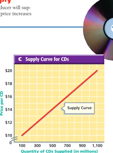
Part A is the supply schedule, or table, showing that as the price per CD increases, the quantity supplied increases. Part B of

Price per CD Points in Part B Quantity supplied (in millions) $10 $11 $12 $13 $14 $15 $16 $17 $18 $19 $20 100 200 300 400 500 600 700 800 900 1,000 1,100 L M N O P Q R S T U V A Supply Schedule for CDs

Part A Supply Schedule The numbers in the supply schedule above show that as the price per CD increases, the quantity supplied increases. Note that at $16 each, a quantity of 700 CDs will be supplied.

Supply Can Be Shown

Visually

Note how the three parts use a different format to show the same thing. Each shows the law of supply—as price rises, quantity supplied increases.

Graphing the Supply Curve

188 C H A P T E R 7

FIGURE 7.8

(24)

supply curve: upward-sloping line that shows in graph form the quantities supplied at each possi-ble price

Figure 7.8is a graph plotting the price and quantity supplied pairs from the supply schedule. Note that the bottom axis shows the quantity supplied. The side axis shows the price per CD. Each intersection of price and quantity supplied represents a point on the graph. We label these points L through V.

When we connect the points from Part B with a line, we end up with the supply curve, as shown in Part C. A supply curve shows the quantities supplied at each possible price. It slopes upward from left to right. You can see that the relationship between price and quantity supplied is direct—or moving in the same direction.

Quantity Supplied vs. Supply

Each point on a supply curve signifies that a producer will sup-ply a certain quantity at each particular price. If the price increases

L M N O P Q R S T U V 100 1,100 Price per CD $20 $18 $16 $14 $12 $10

Quantity of CDs Supplied (in millions)

300 500 700 900 B Plotting the Price –Quantity Pairs

0

Part B Plotting Quantity Supplied Note how the price and quantity supplied numbers in the supply schedule (Part A) have been transferred to a graph in Part B above. Find letter R. Note that it represents a number of CDs supplied (700) at a specific price ($16).

Part C Supply Curve The points in Part B have been connected with a line in Part C above. This line is the supply curve, which always rises from left to right. How many CDs will be supplied at a price of $14 each? 100 1,100 Price per CD $20 $18 $16 $14 $12 $10

Quantity of CDs Supplied (in millions)

300 500 700 900 0

C Supply Curve for CDs

(25)

or decreases, the quantity supplied also increases or decreases. A change in quantity supplied is caused by a change in price and is shown as a movement along the supply curve.

Sometimes, however, producers will supply more goods or fewer goods at every possible price. This is shown as a movement of the entire supply curve and is known as a change in supply. A

change in price does not cause this movement. What does cause

the entire supply curve to shift to the right (increase in supply) or the left (decrease in supply)?

The Determinants of Supply

Four of the major determinants of supply (not quantity supplied) are the price of inputs, the number of firms in the industry, taxes, and technology.

Price of Inputs

If the price of inputs—raw materials, wages, and so on—drops, a producer can supply more at a lower produc-tion cost. This causes the supply curve to shift to the right. This sit-uation occurred, for example, when the price of memory chips fell during the 1980s and 1990s. More computers were supplied at any given price than before. See Part A of Figure 7.9.In contrast, if the cost of inputs increases, suppliers will offer fewer goods for sale at every possible price.

Number of Firms in the Industry

As more firms enter an industry, greater quantities are supplied at every price, and the sup-ply curve shifts to the right. Consider the number of video rentals. As more video rental stores pop up, the supply curve for video rentals shifts to the right. See Part B of Figure 7.9.

Taxes

If the government imposes more taxes, businesses will not be willing to supply as much as before because the cost of production will rise. The supply curve for products will shift to the left, indicating a decrease in supply. For example, if taxes on silk increased, silk businesses would sell fewer quantities at each and every price. The supply curve would shift to the left, as shown in Part C of Figure 7.9.

Technology

The use of science to develop new products and new methods for producing and distributing goods and services is called technology. Any improvement in technology will increase

supply, as shown in Part D.Why? New technology usually reduces

the cost of production. See Figure 7.10 on page 192.

190 C H A P T E R 7

technology: any use of land, labor, and capital that produces goods and services more efficiently

(26)

100 200 300 400 500

Price per Scarf

$120

$90

$60

$30

Quantity of Scarves Supplied S2 S1

C If Taxes Increase

1 2 3 4 5 6 7

Price per Automobile (in $1,000s)

$35 $30 $25 $20 $15 $10

Quantity of Autos Supplied (in 1,000s)

D If Technology Improves Production

S1 S2

Part B Change in Supply if Number of Firms Increases Overall supply will increase if the number of firms in an industry grows. As profits from movie and game rentals increased, for example, the number of video stores supplying these items increased. With more video stores, the supply curve for video rentals increased from S1 to S2.

Part C Change in Supply if Taxes Increase Line S1 indicates the supply of silk scarves beforethe government raised taxes on this business. Line S2 equals the supply afterthe government raised taxes.

Part D Change in Supply if Technology Reduces Costs of Production Any improvement in technology will increase supply—or move the supply curve to the right from S1 to S2. Technology reduces the costs of production, allowing suppliers to make more goods for a lower cost.

100 200 300 400 500

Price per Computer

$2,000 $1,500 $1,000 $500

Quantity of Computers Supplied S1 S2

A If Inputs Become Cheaper

Part A Change in Supply if Price of Inputs Drops

Line S1 shows the supply of computers before the price of memory chips fell. Line S2 shows the increased supply of computers after the price of memory chips fell.

1 2 3 4 5 6 Price per V ideo Rental $3.50 $3.00 $2.50 $2.00 $1.50 $1.00

Quantity of Video Rentals Supplied S2

S1

B If Number of Firms Increases

Changes in Supply

Four major factors affect the supply for a specific product. When supply changes, the entire supply curve shifts to the left or the right.

Determinants of Supply

FIGURE 7.9

(27)

The Law of Diminishing Returns

You want to expand production. Assume you have 10 machines and employ 10 workers. You hire an eleventh worker. CD produc-tion increases by 1,000 per week. When you hire the twelfth worker, CD production might increase by only 900 per week. There are not enough machines to go around, and perhaps work-ers are getting in each other’s way.

This example illustrates the law of diminishing returns.

According to this law, adding units of one factor of production to all the other factors of production increases total output. After a certain point, however, the extra output for each additional

unit hired will begin to decrease.

Technology

In the early 1900s, improved technology for making auto-mobiles drastically reduced the amount of time and other resources it took to make many new automobiles.

Therefore, a larger supply of autos was offered for sale at every price.

1. Define law of supply, quantity supplied, supply schedule, supply curve, technology, law of diminishing returns.

Reviewing Objectives

2.What does the law of supply state?

3.How does the incentive of greater profits affect supply?

4.What do a supply schedule and a supply curve show?

5. Graphic Organizer Create a diagram like the one in the next column to explain the four deter-minants of supply.

6. Supply List at least 10 costs of production if you were to produce and distribute baseball caps to local stores.

7. Synthesizing Information Assume that you are a successful baseball cap maker. Draw a graph that shows the various prices and quantities supplied for your caps.

3

Supply

192 C H A P T E R 7

7.10

key skills with Skillbuilder Interactive Workbook, Level 2. law of diminishing returns:

economic rule that says as more units of a factor of production (such as labor) are added to other factors of production (such as equipment), after some point total output continues to increase but at a diminishing rate

(28)

Understanding cause and effect involves considering why an event occurred. A cause is the action or situation that produces an event. What happens as a result of a cause is an effect.

Critical Thinking Skills

Understanding Cause

and Effect

• Identify two or more events or developments. • Decide whether one event

caused the other. Look for “clue words” such as

because, led to, brought about, produced, as a result of, so that, since,

and therefore.

• Look for logical relation-ships between events, such as “She overslept, and then she missed her bus.”

• Identify the outcomes of events. Remember that some effects have more than one cause, and some causes lead to more than one effect. Also, an effect can become the cause of yet another effect.

Learning the Skill

To identify cause-and-effect relationships, follow the steps listed on the left.

Practicing the Skill

The classic cause-and-effect relationship in econom-ics is between price and quantity demanded/quantity supplied. As the price for a good rises, the quantity demanded goes down and the quantity supplied rises.

1. Look at Figure A. What caused the big sale? What

is the effect on consumers?

2. Look at the demand curve for DVD systems in

Figure B. If the price is $5,000, how many will be demanded per year? If the price drops to $1,000, how many will be demanded per year?

BIG SALE!

PRICES

SLASHED!

Huge inventory needs

to be sold to make room for next

year’s model. 5 4 3 2 1 0 1 2 3 4 5 Quantity demanded (in millions) Price (in $1,000s) Figure A Figure B

Application Activity

In your local newspaper, read an article describing a current event. Determine at least one cause and one effect of that event.

(29)

194 C H A P T E R 7 Terms to Know •equilibrium price •shortage •surplus •price ceiling •rationing •black market •price floor Reading Objectives

1.How is the equilibrium price determined?

2.How do shifts in equilibrium price occur?

3.How do shortages and sur-pluses affect price? 4.How do price ceilings and

price floors restrict the free exchange of prices?

R

EADER

’

S

G

UIDE

W

hat do Furbys™, Beanie Babies™, Tickle Me Elmo™,

and Cabbage Patch Kids™ all have in common? At one point in time, they all were in short supply—and usually right before the Christmas holiday season. As you will read, shortages occur when the quantity demanded is larger than the quantity supplied at the current price.

Equilibrium Price

In the real world, demand and supply operate together. As the price of a good goes down, the quantity demanded rises and the

TIME, NOVEMBER 30, 1998

Your kid won’t stop begging for a Furby, right? . . . And you’ve driven to every mall in the

state and still can’t find it. Your next-door neighbor traded his car for a dozen on a black-market website, but he’s hoarding them until just before Christmas, prime time for scalping. You’re stuck with a K Mart waiting list and cheerful lies from salespeople: “We’ll call you soon.” Makes you wanna gouge those adorable Furby eyes right out of their electronic sockets.

4

(30)

equilibrium price: the price at which the amount producers are willing to supply is equal to the amount consumers are willing to buy

quantity supplied falls. As the price goes up, the quantity demanded falls and the quantity supplied rises.

Is there a price at which the quantity demanded and the quan-tity supplied meet? Yes. This level is called the equilibrium price. At this price, the quantity supplied by sellers is the same as the quantity demanded by buyers. One way to visualize equilibrium price is to put supply and demand curves on one graph, as shown in Figure 7.11. Where the two curves intersect is the equilibrium price. At that price, shown in the graph above, the quantity of CDs that consumers are willing and able to purchase is 600 million per year. And suppliers are willing to supply exactly that same amount.

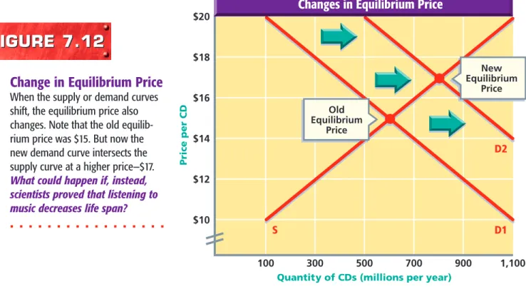
Shifts in Equilibrium Price

What happens when there is an increase in the demand for CDs? Assume that scientists prove that listening to more music increases life span. This discovery will cause the entire demand curve to shift outward to the right, as shown in Figure 7.12 on page 196.

What about changes in supply? You can show these in a similar fashion. Assume that there is a major breakthrough in the technol-ogy of producing CDs. The supply curve shifts outward to the right. The new equilibrium price will fall, and both the quantity suppliedand the quantity demandedwill increase.

Equilibrium Price

In a market economy, the forces underlying demand and sup-ply have a push-pull relation-ship that ultimately leads to an equilibrium price. In our particular example, this is $15 per CD. If the price were to go above $15, the quantity demanded would be less than the quantity supplied. If the price fell below $15 per CD, the quantity demanded would exceed the quantity supplied.

100 300 500 700 900 1,100 Price per CD $20 $18 $16 $14 $12 $10

Quantity of CDs (millions per year)

S D

Equilibrium Price Graphing the Equilibrium Price

FIGURE 7.11

(31)

196 C H A P T E R 7

shortage: situation in which the quantity demanded is greater than the quantity supplied at the current price

surplus: situation in which tity supplied is greater than quan-tity demanded at the current price

Prices Serve as Signals

In the United States and other countries with mainly free enter-prise systems, prices serve as signals to producers and consumers. Rising prices signal producers to produce more and consumers to purchase less. Falling prices signal producers to produce less and consumers to purchase more.

Shortages

A shortage occurs when, at the current price, the quantity demanded is greater than the quantity supplied. If the market is left alone—without government regulations or other restrictions—shortages put pressure on prices to rise. At a higher price, consumers reduce their purchases, whereas suppliers increase the quantity they supply.

Surpluses

At prices above the equilibrium price, suppliers pro-duce more than consumers want to purchase in the marketplace.

Suppliers end up with surpluses—large inventories

of goods—and this and other forces put pressure on the price to drop to the equilibrium price. If the price falls, suppliers have less incentive to supply as much as before, whereas consumers begin to purchase a greater quantity. The decrease in price toward the equilibrium price, therefore, eliminates the surplus.

100 300 500 700 900 1,100 Price per CD $20 $18 $16 $14 $12 $10

Quantity of CDs (millions per year)

S D1 D2 New Equilibrium Price Old Equilibrium Price

Changes in Equilibrium Price

Change in Equilibrium Price

When the supply or demand curves shift, the equilibrium price also changes. Note that the old equilib-rium price was $15. But now the new demand curve intersects the supply curve at a higher price—$17.

What could happen if, instead, scientists proved that listening to music decreases life span?

FIGURE 7.12

(32)

Market Forces

One of the benefits of the market economy is that when it operates without restriction, it eliminates shortages and surpluses. Whenever shortages occur, the market ends up tak-ing care of itself—the price goes up to eliminate the shortage. Whenever surpluses occur, the market again ends up taking care of itself—the price falls to eliminate the surplus. Let’s take a look at what happens to the availability of goods and services when the government—not market forces—becomes involved in setting prices.

Price Controls

Why would the government get involved in setting prices? One reason is that in some instances it believes the market forces of sup-ply and demand are unfair, and it is trying to protect consumers and suppliers. Another reason is that special interest groups use pressure on elected officials to protect certain industries.

Price Ceilings

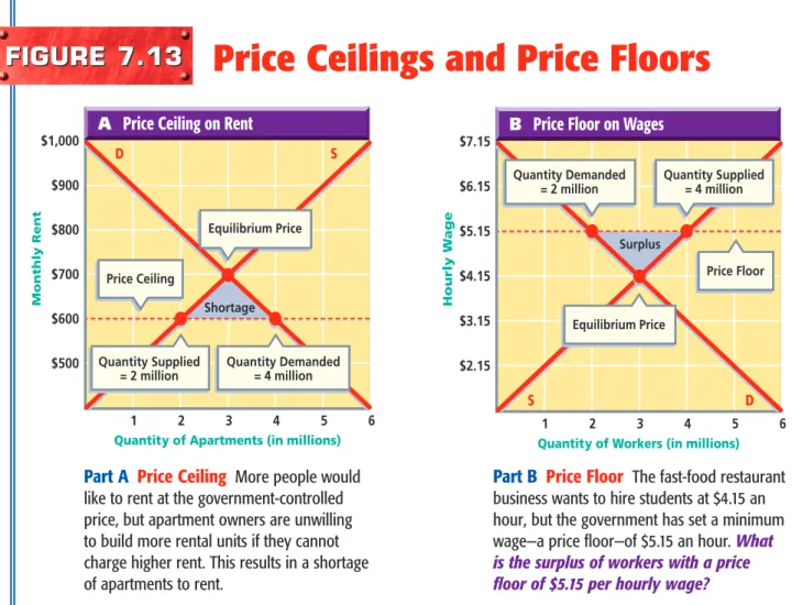
A price ceiling is a government-set maximum price that can be charged for goods and services. Imagine trying to bring a 12-foot tree into your house that has 8-foot ceilings. The ceiling prevents the top of the tree from going up. Similarly, a

price ceiling prevents prices from going above a specified amount. For example, city officials might set a price ceiling on what land-lords can charge for rent. As Part A of Figure 7.13 on page 198 shows, when a price ceiling is set below the equilibrium price, a shortage occurs.

Effective price ceilings—and resulting shortages—often lead to nonmarket ways of distributing goods and services. The govern-ment may resort to rationing, or limiting, items that are in short supply. A policy of rationing is expensive, however. Taxpayers must pay the cost of printing ration coupons, setting up offices to distribute the coupons, and maintaining the bureaucracy involved in enforcing who gets how much of the rationed goods.

Shortages also may lead to a black market, in which illegally high prices are charged for items that are in short supply. As

Figure 7.14 on page 199 shows, items often sold on the black market include tickets to sporting events.

price ceiling: a legal maximum price that may be charged for a particular good or service

rationing: the distribution of goods and services based on something other than price black market: “underground” or illegal market in which goods are traded at prices above their legal maximum prices or in which ille-gal goods are sold

Surplus Cheese

(33)

price floor: a legal minimum price below which a good or serv-ice may not be sold

Price Floors

A price floor, in contrast, is a government-set

minimum price that can be charged for goods and services. Price floors—more common than price ceilings—prevent prices from dropping too low. When are low prices a problem? Assume that about 30 of your classmates all want jobs after school. The local fast-food restaurant can hire 30 students at $4.15 an hour, but the government has set a minimum wage—a price floor—of $5.15 an hour. Some of you will get hired, and you’ll happily earn $5.15 an hour. Not all of you will get hired at that wage, however, which leads to a surplus of unemployed workers as shown in Part B of

Figure 7.13. If the market were left on its own, the equilibrium price of $4.15 per hour would have all of you employed.

Besides affecting the minimum wage, price floors have been used to support agricultural prices. If the nation’s farmers have a bumper crop of wheat, for example, the country has a huge sur-plus of wheat. The market, if left alone, would take care of the

1 2 3 4 5 6 Hourly W age $7.15 $6.15 $5.15 $4.15 $3.15 $2.15 Surplus

Quantity of Workers (in millions)

D S Price Floor Quantity Supplied = 4 million Quantity Demanded = 2 million Equilibrium Price B Price Floor on Wages

Shortage 1 2 3 4 5 6 Monthly Rent $1,000 $900 $800 $700 $600 $500

Quantity of Apartments (in millions)

D S Price Ceiling Quantity Supplied = 2 million Quantity Demanded = 4 million Equilibrium Price A Price Ceiling on Rent

Part A Price Ceiling More people would like to rent at the government-controlled price, but apartment owners are unwilling to build more rental units if they cannot charge higher rent. This results in a shortage of apartments to rent.

Part B Price Floor The fast-food restaurant business wants to hire students at $4.15 an hour, but the government has set a minimum wage—a price floor—of $5.15 an hour. What is the surplus of workers with a price floor of $5.15 per hourly wage?

Price Ceilings and Price Floors

FIGURE 7.13

(34)

surplus by having the price drop. As prices decrease, remember, quantity supplied decreases and quantity demanded increases. But the nation’s farmers might not earn enough to make a profit or even pay their bills if the price drops too much. So the government sometimes sets a price floor for wheat, which stops the price per bushel from dropping below a certain level. The farmers know this, so instead of reducing their acreage of wheat—which would reduce the surplus—they keep producing more wheat.

Black Market

Scalpers selling high-priced, limited tickets—such as these tick-ets to a World Cup Soccer match—are part of the black market. How do price ceil-ings on tickets to sporting events lead to shortages?

7.14

1. Define equilibrium price, shortage, surplus, price ceiling, rationing, black market, price floor. Reviewing Objectives

2.How is the equilibrium price determined?

3.How do shifts in equilibrium price occur?

4. Graphic Organizer Create a diagram like the one below to show how shortages and sur-pluses affect prices.

5.How do price ceilings and price floors restrict the free exchange of prices?

6. Shortages Explain how a shortage of profes-sional sports tickets determines the general price of those tickets.

7. Understanding Cause and Effect Draw a series of three graphs.

•The first graph should show an equilibrium price for sunglasses.

•The second graph should show the shift that would occur if research proved wearing sunglasses increased I.Q.

•The third graph should show the shift that would occur if research proved that wearing sunglasses caused acne. For help in using

graphs, see page xv in the Economic Handbook.

4

Supply Impact on Prices Shortage

(35)

■ _{Began career as a} mathematician ■ Chaired political economy at Cambridge University, England ■ _{Developed supply} and demand analysis ■ _{Published Principles} of Economics (1890) and Elements of Economics (1892)

A

lfred Marshall is known

for introducing the concept of supply and demand analysis to economics. The following excerpt from Elements of Eco-nomics explains the concept of equilibrium:

“

The simplest case of balance, or equilibrium, between desire and effort is found when a person satis-fies one of his wants by his own direct work. When a boy picks blackberries for his own eating, the action of picking may itself be pleasurable for a while. . . .

Equilibrium is reached, when at last his eagerness to play and his disinclination for the work of pick-ing counterbalance the desire for eating. The satisfaction which he can get from picking fruit has arrived at its maximum. . . .

”

Marshall also explained how equilibrium is established in a local market. Buyers and sellers, having perfect knowledge of the market, freely compete for their

own best interests. In so doing they arrive at a price that exactly equates supply and demand.

“

. . . [A price may be] called the true equilibrium price: because if it were fixed on at the beginning, and adhered to throughout, it would exactly equate demand and supply. (i.e. the amount which buy-ers were willing to purchase at that price would be just equal to that for which sellers were willing to take that price). . . .

In our typical market then we assume that the forces of demand and supply have free play; that there is no combination among dealers on either side; but each acts for himself, and there is much free competition; that is, buyers gener-ally compete freely with buyers, and sellers compete freely with sellers.

”

Checking for Understanding

1. What does Marshall mean by “equi-librium between desire and effort”?

2. What is an equilibrium price?