Bias in regression coefficient estimates when
assumptions for handling missing data are
violated: a simulation study
ABSTRACT
Background: The purpose of this simulation study is to compare bias in the estimation of regression coefficients between multiple imputation (MI) and complete case (CC) analysis when assumptions of missing data mechanisms are violated.
Methods: The authors performed a stochastic simulation study in which data were drawn from a multivariate normal distribution, and missing values were created according to different missing data mechanisms (missing completely at random (MCAR), at random (MAR), and not at random (MNAR)). Data were analysed with a linear regression model using CC analysis, and after MI. In addition, characteristics of the data (i.e. correlation, size of the regression coefficients, error variance, proportion of missing data) were varied to assess the influence on the size and sign of bias.
Results: When data were MAR conditional on Y, CC analysis resulted in severely biased regression coefficients; they were consistently underestimated in our scenarios. In the same scenarios, analysis after MI gave correct estimates. Yet, in case of MNAR MI yielded biased regression coefficients, while CC analysis did not result in biased estimates, contrary to expectation.
Conclusion: The authors demonstrated that MI was only superior to CC analysis in case of MCAR or MAR, with respect to bias and precision. In some scenarios CC may be superior to MI. Often it is not feasible to identify the cause of incomplete data in a given dataset. Therefore, emphasis should be placed on reporting the extent of missing values, the method that was used to address the problem, and the assumptions that were made about the mechanism that caused missing data.
Key words: multiple imputation, complete case analysis, missing data, bias, regression
Sander MJ van Kuijk (1,2), Wolfgang Viechtbauer (3), Louis L Peeters (4), Luc Smits (2)
(1) Clinical Epidemiology and Medical Technology Assessment, Maastricht University Medical Centre, Maastricht, The Netherlands (2) Epidemiology, Maastricht University, PO Box 616, 6200 MD, Maastricht, The Netherlands
(3) Statistics and Methodology, Maastricht University, PO Box 616, 6200 MD, Maastricht, The Netherlands
(4) Obstetrics & Gynecology, Maastricht University Medical Centre, PO Box 5800, 6202 AZ, Maastricht, The Netherlands
CORRESPONDING AUTHOR: Sander van Kuijk, PhD, Department of Clinical Epidemiology and Medical Technology Assessment, Maastricht University Medical Centre, P. Debyelaan 25, PO box 5800, 6202 AZ Maastricht.
Phone: +31 043 3874374; Fax: 043-3874419; E-mail: [email protected]
DOI: 10.2427/11598
Accepted on December 28, 2015
INTRODUCTION
One of the most ubiquitous problems in epidemiological studies is that of missing values. The standard approach to handling missing values for most statistical packages,
analysis than planned. Moreover, CC analysis may cause considerable bias in the parameter estimates [1-4].
The extent of the problem has been widely acknowledged for decades by statisticians and many methods to deal with missing values have been developed since. Most methods aim to impute values, providing the analyst with a complete dataset. These methods make specific assumptions about the mechanism(s) that caused the data to be missing. An increasingly popular imputation method among researchers is Multiple Imputation (MI) [5]. This method creates multiple completed datasets, usually 5, 10, or more. For each dataset, missing values are estimated using regression, or predictive mean matching (i.e. a value is drawn at random from a set of donors with predicted values close to the predicted value for the incompletely observed record), or another method, and always introduces a stochastic element that creates inter-dataset variability. Pooling results from these datasets produces estimates that have correct standard errors [2-4,7]. As used in practice, MI usually assumes data are either MCAR or missing conditional on the value of other variables in the model, including the outcome variable. The latter mechanism is called Missing at Random (MAR) [6]. For circumstances in which the MCAR or MAR assumption is met, MI has been shown to be superior to other popular imputation methods such as imputation with the (conditional) mean, the missing-indicator method, last observation carried forward, and single imputation.
The use of any method for handling missing data can introduce bias if the missing data assumptions are not met. However, it is not customary that such methods are reported in detail, and if they are, the authors usually do not provide convincing support for the validity of the assumptions [8]. A third and more problematic missing data mechanism is often overlooked, namely Missing Not at Random (MNAR), in which values are missing conditional on their own true value or the value of covariates that are unmeasured.
In a recent simulation study, White and Carlin [9] showed that when data are not MCAR, there are some scenarios in which a CC analysis yields negligible bias while MI can introduce considerable bias when estimating coefficients of a regression model. They also provide an index for assessing the likely gain in precision from MI. These findings raise some doubt about the routine application of MI as a panacea for dealing with missing data.
In the present article, we focused on bias in the estimation of regression coefficients after MI as compared to CC analysis in scenarios when assumptions were violated, with particular emphasis on scenarios that have received little attention in other simulation studies. Furthermore, we assessed which parameters of the regression model determined the extent of the bias, if any, and whether they influenced the sign of bias. We focused
in particular on MI as the imputation method, since it is commonly considered to be superior to other popular methods. To compare MI with CC analysis, we performed a Monte Carlo simulation study.
METHODS
Study design
We performed a Monte Carlo simulation study to evaluate properties of MI and CC in several missing data scenarios. We simulated data based on a linear model given by
Y = β0 + β1X1 + β2X2 + ε (1)
in which Y is the continuous outcome variable, X1 and
X2 are both continuous independent variables, β0 is the intercept, and X1 and X2 denote the regression coefficients for the corresponding X variables, and ε is the error variable (or residual). The independent variables as well as the error variable were drawn from a multivariate normal distribution with zero means, unit variances and correlation between the independent variables equal to p. The errors were drawn from an independent normal distribution with zero mean and variance equal to σ2. The model intercept,
β0, was set to 0.
To determine the influence of sample size (n), the error variance (σ2), the correlation between the independent
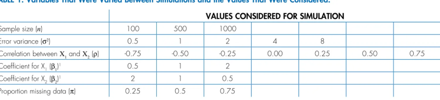
variables (p), and the size of the regression coefficients relative to one another (β1 and β2), we varied all these factors throughout the simulation study. Table 1 shows all the values considered for the different simulations. This amounts to 315 different scenarios of complete data.
Creation of missing values
We created missing values on the X1 variable according to the MCAR, MAR and the MNAR mechanisms. For the MCAR mechanism, a randomly selected proportion of X1 was deleted, independent of the values of any other variable in the model. This was done by simulating a variable from a Bernoulli distribution of the same size as X1, with a probability of success (i.e. the value = 1) equal to the proportion missing values according to the scenario. For each value of the Bernoulli-distributed variable that was ‘1’, the corresponding X1 value was deleted.
The MAR mechanism was divided into MAR conditional on the X2 variable (i.e. the lower the X2
value, the higher the probability that the corresponding
deviation unity and a mean determined by the proportion of missing values that particular scenario dictated. This variable was compared either to X2 or Y, depending on the missing value mechanism. If the value of the random variable was lower than the corresponding X2 or Y, the corresponding X1 value was not manipulated, if it was higher the X1 value deleted.
To simulate a MNAR mechanism, the probability for any value to be missing was associated with its own value (i.e., the lower the value, the higher the probability of being missing). We created these missing values similar to the MAR mechanism. In this case, the normally distributed variable was compared to X1, as opposed to X2 or Y. These 4 mechanisms were applied separately to all 315 datasets. Furthermore, we varied the proportion of missing values in all datasets (π). We created missing values in proportions of 0.25, 0.50 and 0.75. Therefore, a total of 315 * 4 * 3 = 3.780 different conditions were examined in this simulation study.
Data analysis
We analysed all these scenarios using both CC analysis and after MI using linear regression analysis to estimate regression coefficients. The linear model that was analysed was of the same structure as {1}. MI was performed using the mice package (Multiple Imputation using Chained Equations), which was developed by the Netherlands Organization for Applied Scientific Research (TNO) [10]. The default settings were used, which means that the imputations were generated using the frequently employed method of predictive mean matching, and the number of multiple imputations was set to 5. All simulations were performed 1,000 times to obtain stable estimates of regression coefficients and standard errors. R [11] was used for simulating the data and performing all analyses.
RESULTS
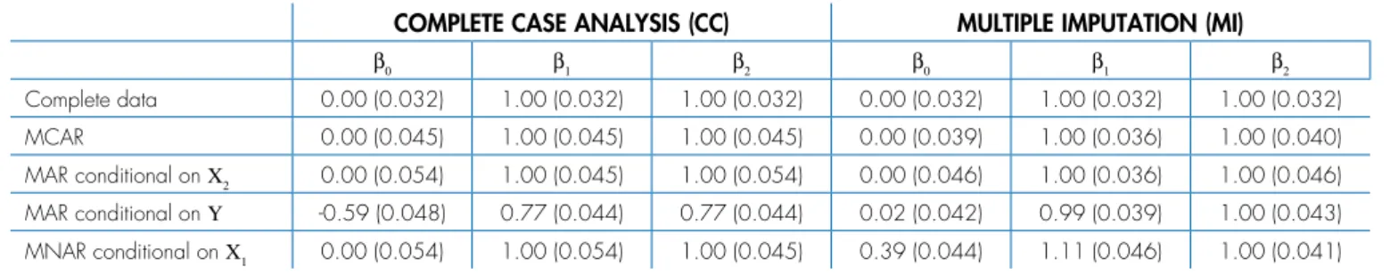
Table 2 shows the mean of the parameter estimates and corresponding standard errors both for the complete
and incomplete data scenarios. The incomplete data were analysed using CC analysis and analysis after MI. All scenarios reported in table 2 had the following settings: n = 1000, σ2 = 1, β
1 = β2 = 1, p = 0.00,
and π = 0.50.
Complete case analysis
Compared to the results generated for the complete data, standard errors increased with an increasing proportion of missing data. When the MCAR assumption held, regression coefficients were unbiased. Moreover, when data were MAR, conditional on X2, or when data were MNAR, conditional on its own true value, CC analysis also yielded unbiased regression parameter estimates. Only when data were MAR, conditional on the outcome variable Y, CC analysis resulted in biased estimates. Both regression coefficients were underestimated, with the intercept being overestimated.
Multiple Imputation
When data were MCAR or MAR, which is an assumption of MI, the analysis yielded unbiased parameter estimates. The standard errors were slightly higher than those computed on the complete data, because the uncertainty of imputation was taken into account. When the MAR assumption was violated (i.e. MNAR), analysis after MI overestimated the regression coefficient of X1, and underestimated the intercept. The regression coefficient of
X2, however, was unbiased.
Influence of model parameters
The following results describe conditions in which the sample size n was 1000 and, unless otherwise stated, the true values of the regression coefficients β1 and β1 were 1, the error variance was 1, the proportion of missing values was 0.5 and the correlation between the independent variables was 0.
VALUES CONSIDERED FOR SIMULATION
Sample size (n) 100 500 1000
Error variance (σ2) 0.5 1 2 4 8
Correlation between X1 and X2 (ρ) -0.75 -0.50 -0.25 0.00 0.25 0.50 0.75
Coefficient for X1 (β1)1 0.5 1 2
Coefficient for X2 (β2)1 2 1 0.5
Proportion missing data (π) 0.25 0.5 0.75
1Not all possible combinations of the regression coefficients were considered, only (β
CC analysis when data are MAR conditional on Y
Figure 1(a-f) shows the influence of model parameters on scenarios in which CC analysis yielded biased results, namely when data were missing at random, conditional on the dependent variable Y. Figure 1a and 1b illustrate that the size of bias in the estimated intercept was greatly influenced by the variance in the error term and consequently the variance of Y. Furthermore, the size of bias was proportional to the proportion of missing values of the X1 variable. The correlation between predictor variables and the true values of the regression coefficients seems to have had no influence on the bias of the mean intercept estimate.
Figures 1c and 1d show the size of the estimated regression coefficient of X1, (i.e. β1). The same conclusions hold as for the estimation of the intercept, but now the correlation between the independent variables X1 and
X2 also influenced bias. The bias was highest with a high negative correlation, and lowest with a high positive correlation. The relation seemed linear within the simulated range. Figure 1d illustrates that the bias depended on the true value of the regression coefficient; it was proportional to its size.
Figure 1e and 1f show the estimation of the regression coefficient β2. For both graphs, the same conclusions can be drawn as for the estimation of the regression coefficient for X1. In our scenarios considering MAR, conditional on the dependent variable Y, CC analysis consistently underestimated the regression coefficients and thus resulted in a negative bias.
Analysis after MI when data are MNAR conditional on X1
Figure 2(a-f) shows the influence of model parameters on scenarios in which analysis after MI yielded biased results, namely when data were missing not at random, conditional on the true value of X1. Figure 2a and 2b show the results for the model intercept, revealing that the bias was dependent on the error variance (thus the variance on Y), the correlation between X1 and X2, the proportion of missing values in the X1 variable and the size of the regression coefficients relative to one another. The
bias increased as a function of the variance of the error term. The weaker the correlation between the independent variables was, the larger the bias in the estimation of the intercept. This relationship can be described by a curve (see figure 2a). Just as in the previous examples with CC analysis, the bias increased as a function of the proportion of missing values. Contrary to results from the CC analysis, the true value of the regression coefficients also influenced bias in the estimated intercept.
Figure 2c and 2d show bias in the estimation of the regression coefficient of X1. The results were similar to those of the estimation of the intercept. However, we observed an inverse relation between the error variance and the magnitude of the bias. It shows that the lower the variance was, the higher the bias. Furthermore, instead of an overestimation of the regression coefficient, scenarios with an error variance of 4 or 8, and a correlation between the independent variables of 0.75 showed a slight underestimation of the regression coefficient. Figure 2d shows that the model slightly overestimated the regression coefficients, the size of bias being proportional to the true value. However, in this scenario bias was not that much affected by the proportion of missing values.
Figure 2e and 2f illustrate bias in the estimation of the regression coefficient for X1 when data were missing not at random. Bias increased as a function of error variance. In these scenarios it was evident that the model underestimated the coefficient in case of a negative correlation between X1 and X2, and overestimated in case of a positive correlation. Bias in the estimation of this coefficient was hardly influenced by both the proportion of missing values, and the true value of the coefficient.
DISCUSSION
Our simulations indicate that estimated regression coefficients for incomplete data can be biased using a standard approach like CC analysis, but also when using a sophisticated method like MI. When data were MCAR or MAR, conditional on X2, both methods performed well, although a larger loss of precision when using CC could be observed because of the omission of patients,
COMPLETE CASE ANALYSIS (CC) MULTIPLE IMPUTATION (MI)
β0 β1 β2 β0 β1 β2
Complete data 0.00 (0.032) 1.00 (0.032) 1.00 (0.032) 0.00 (0.032) 1.00 (0.032) 1.00 (0.032)
MCAR 0.00 (0.045) 1.00 (0.045) 1.00 (0.045) 0.00 (0.039) 1.00 (0.036) 1.00 (0.040)
MAR conditional on X2 0.00 (0.054) 1.00 (0.045) 1.00 (0.054) 0.00 (0.046) 1.00 (0.036) 1.00 (0.046)
MAR conditional on Y -0.59 (0.048) 0.77 (0.044) 0.77 (0.044) 0.02 (0.042) 0.99 (0.039) 1.00 (0.043)
MNAR conditional on X1 0.00 (0.054) 1.00 (0.054) 1.00 (0.045) 0.39 (0.044) 1.11 (0.046) 1.00 (0.041)
TABLE 2. Mean of the Regression Coefficient Estimates (and Corresponding Standard Errors) for complete and missing data scenarios in which n = 1000, σ2 = 1, β
Figure 2(a-f). The mean estimated regression coefficients after MI when data are MNAR conditional on X1. To assess the influence of the β2 value and the proportion of missing values on the mean β2 estimate (figure 2f), we set ρ = 0.50, since figure 2E shows no bias
when ρ = 0.00. The dotted line represents the true value of the regression coefficient. The three graphs on the left show the effect of the correlation between X1 and X2, and the variance of the error term, on the bias in the regression coefficients after MI. In the graphs on the right, the proportion of missing values and the size of the regression coefficients were varied.
which holds for all missing data conditions we analysed. Contrary to what we expected, CC analysis only yielded biased regression coefficients when missing data were
MAR conditional on Y. Moreover, when data were
MNAR results obtained after MI were biased whereas CC yielded correct estimates. This is not likely to hold for all possible MNAR mechanisms, but it did hold for all MNAR mechanisms simulated in this study. In scenarios where CC analysis lead to biased results the regression coefficients were consistently underestimated. Conversely, in scenarios where analysis after MI yielded biased results, the regression coefficients were in most cases overestimated. In most of the scenarios we considered, the magnitude of the bias was influenced by the error variance, or the variance on Y, by the correlation between the independent variables, the proportion of missing values and the true value of the regression coefficients β1 and β2.
Relatively little attention has been given to MNAR in other empirical and simulation studies. It is described as unlikely to occur [12], or described as a scenario for which no universal method can provide reliable estimates of regression coefficients [4,6,12,13]. A prime example of data MNAR is the following. Consider a personal question in a survey that people with a particular value or answer are less likely to complete, for instance asking smoking status among pregnant women. Women who still smoke during pregnancy are more likely to skip the question than women who do not smoke. Another example is asking for income or salary, a question less likely to be completed by people with very low or high incomes. When visiting a gynecologist during pregnancy, body mass index (BMI) may be recorded only when it is suspected to be relevant, that is either very low or very high. For clinical laboratory results, MNAR may occur when a ceiling effect is present, i.e. when a level above which a variable cannot be measured is reached, and is therefore not observed.
It follows from our results that determining the missing data mechanisms are crucial for choosing the correct method for handling missing values. Yet it is hard, if not impossible, to prove empirically that one mechanism in particular can be kept responsible for missing data, or to rule out another. It can only be assumed after detailed inspection of the raw data and thinking thoroughly about the data collection procedure. Furthermore, despite the fact that the missing data mechanisms are usually presented as mutually exclusive, it is likely that, in any given large multivariable dataset, combinations of mechanisms can cause incomplete data, presenting the analyst an even more difficult problem deciding what method to use. A result of this could be that imputation methods perform worse in empirical datasets, compared to the many simulation studies performed under perfect circumstances.
One important drawback of our study is that there are many more theoretical scenarios that can be simulated using some sort of MNAR mechanism, which falls well beyond the scope of this article. We emphasise that,
since these were not simulated, we cannot generalise our results to these many scenarios. This also holds for scenarios in which the model is expanded with more covariates, interaction terms, multilevel structure, or other features. Yet, we aimed to present a simple simulation for illustrative purposes, and discussing many more missing data mechanisms is unlikely to alter our conclusion.
An important improvement would be if authors of empirical articles put more emphasis on the absolute number and proportion of missing values and the missing data. Stating how many patients will be omitted from the analysis if CC analysis is used and how many values are missing on each variable of interest, are of great importance for the interpretation of the results. A sound description of the assumptions that were made and why, and the method or methods chosen for handling these missing values should follow, providing the interested reader with sufficient information to determine the validity of the results in the context of the research question addressed. Any differences between results obtained after CC analysis and analysis after MI could provide insight in the stability of the results.
CONCLUSION
In conclusion, this paper does not intend to discourage the use of MI or CC analysis for that matter. However, we intended to demonstrate the importance of keeping in mind that MI has some pitfalls, and CC analysis may provide valid results in some scenarios where MI fails to do so. An uncertainty is always introduced when missing values are present, and the data analyst should realize that in this case, data used for the analyses never equal the data as they were collected, whatever method is used. Therefore, one should always give enough information for the reader to get an impression of the extent of the problem.
Acknowledgements
We thank our colleagues of the Clinical Epidemiology Research Program at Maastricht University Medical Centre for sharing their insights during the methodology focus meetings.
References
1. van der Heijden GJ, Donders AR, Stijnen T, Moons KG. Imputation of missing values is superior to complete case analysis and the missing-indicator method in multivariable diagnostic research: a clinical example. J Clin Epidemiol 2006; 59:1102-9.
2. Allison PD. Missing Data. Iowa: Sage, 2001.
3. Steyerberg EW. Clinical Prediction Models. New York: Springer; 2009. 4. Harrell Jr FE. Regression Modeling Strategies. New York: Springer;
5. Schafer JL. Multiple imputation: a primer. Stat Methods Med Res 1999; 8:3-15.
6. Rubin DB. Inference and missing data. Biometrika 1976; 63:581-92. 7. Janssen KJ, Vergouwe Y, Donders AR, et al. Dealing with missing
predictor values when applying clinical prediction models. Clin Chem 2009; 55:994-1001.
8. Fernandes-Taylor S, Hyun JK, Reeder RN, Harris AH. Common statistical and research design problems in manuscripts submitted to high-impact medical journals. BMC Res Notes 2011;4:304. 9. White IR, Carlin JB. Bias and efficiency of multiple imputation
compared with complete-case analysis for missing covariate values. Stat Med 2010;29:2920-31.
10. van Buuren S, Oudshoorn CGM. Multivariate Imputation by Chained Equations. MICE V1.0 User’s manual. TNO report PG/ VGZ/00038. 2000.
11. R Development Core Team (2008). R: A language and environment for statistical computing. R Foundation for Statistical Computing, Vienna, Austria. ISBN 3-900051-07-0, Available from http://www.R-project. org.
12. Schafer JL. Analysis of incomplete multivatiate data. London: Chapman &Hall/CRC Press, 1997.