Relative Merits of 3D Visualization for the Detection of Subtle Lung Nodules
Sarah Jonathan Boyce
A dissertation submitted to the faculty of the University of North Carolina at Chapel Hill in partial fulfillment of the requirements for the degree of Doctor of Philosophy in the Department of Biomedical Engineering
Chapel Hill 2013
Approved by:
Ehsan Samei, PhD
David Lalush, PhD
Marija Ivanovic, PhD
Henry Hsiao, PhD
©2013
iii ABSTRACT
SARAH BOYCE: Relative Merits of 3D Visualization for the Detection of Subtle Lung Nodules. (Under the direction of Ehsan Samei)
A new imaging modality called bi-plane correlation imaging (BCI) was examined
to determine the merits of using BCI with stereoscopic visualization to detect subtle lung
nodules. In the first aim of this project, the optimal geometry for conventional projection
imaging applications was assessed using a theoretical model to develop generic results
for MTF, NNPS, eDQE. The theoretical model was tested with a clinical system using
two magnifications and two anthropomorphic chest phantoms to assess the modalities of
single view CXR and stereo/BCI. Results indicated that magnification can potentially
improve the signal and noise performance of digital images. Results also demonstrated
that a cross over point occurs in the spatial frequency above and below which the effects
of magnification differ indicating that there are task dependent tradeoffs associated with
magnification. Results indicated that magnification can potentially improve the detection
performance primarily due to the air gap which reduced scatter by 30-40%. For both
anthropomorphic phantoms, at iso-dose, eDQE(0) for stereo/BCI was ~100 times higher
than that for CXR. Magnification at iso-dose improved eDQE(0) by ~10 times for BCI.
Increasing the dose did not improve results. The findings indicated that stereo/BCI with
magnification may improve detection of subtle lung nodules compared to single view
With quantitative results in place, a pilot clinical trial was constructed. Human
subject data was acquired with a BCI acquisition system. Subjects were imaged in the
PA position as well as two oblique angles. Realistic simulated lesions were added to a
subset of subjects determined to be nodule free. A BCI CAD algorithm was also applied.
In randomized readings, radiologists read the cases according to viewing protocol. For
the radiologist trainees, the AUC of lesion detection was seen to improve by 2.8% (p <
0.05) for stereoscopic viewing after monoscopic viewing compared to monoscopic
viewing only. A 13% decrease in false positives was observed.
Stereo/BCI as an adjunct modality was beneficial. However, the full potential of
stereo/BCI as a replacement modality for single view chest x-ray may be realized with
improved observer training, clinically relevant stereoscopic displays, and more
v
DEDICATION
To daddy, for your unconditional love, your unwavering faith in my abilities, your
ACKNOWLEDGEMENTS
I would like to thank my husband and children for their love and support
throughout this long process.
Many, many thanks to Ehsan Samei for allowing me to study under his expert
guidance and for his patient support.
I would also like to thank Varian Medical Systems, Inc. for equipment and for my
co-workers there who inspired me to achieve this milestone. A special thank you to Rick
Harris, if he had not hired me, I never would have started the journey.
Thank you to Planar Systems, Inc. for equipment used in this study. Thanks are
also due to Robert Saunders and Brian Harrawood for image analysis routines. The
author would like to thank Anne Jarvis, Brenda Prince, Rob Saunders, Ben Pollard, Amar
Chawla and Xiang Li for help coordinating the clinical trial as well as Nicole Ranger and
Jin Wooi Tan for coordinating the observer study. Than you to Michael Flynn of Henry
Ford Health Systems, Detroit, MI for tshow software to optimize images for display and
vii
TABLE OF CONTENTS
ABSTRACT ... iii
LIST OF TABLES ...x
LIST OF FIGURES ... xi
ABBREVIATIONS ... xiv
1 Introduction ...1
1.1 CHALLENGES OF CHEST IMAGING ...1
1.2 DIGITAL DETECTOR TECHNOLOGY ...4
1.3 COMPUTED RADIOGRAPHY ...5
1.4 CCD/CMOS DETECTORS ...7
1.5 FLAT PANEL DETECTORS ...7
1.6 PHOTON COUNTING DETECTORS ...11
1.7 COMPUTER AIDED DETECTION ...12
1.8 APPLICATIONS FOR CHEST IMAGING ...13
1.9 SLOT-SCANNING SYSTEMS ...14
1.10 DUAL-ENERGY SYSTEMS ...15
1.11 TOMOSYNTHESIS SYSTEMS ...16
1.12 BI-PLANE CORRELATION SYSTEMS ...17
1.13 OBJECTIVES AND ORGANIZATION ...19
2 Imaging properties of digital magnification radiography ...21
2.2 METHODS ...22
2.3 RESULTS ...30
2.4 DISCUSSION ...41
2.5 CONCLUSION ...44
3 Physical evaluation of a high frame rate, extended dynamic range flat panel detector for real-time cone beam computed tomography applications ...45
3.1 INTRODUCTION ...45
3.2 METHODS ...45
3.3 RESULTS ...50
3.4 DISCUSSION ...56
3.5 CONCLUSION ...57
4 Effective DQE (eDQE) for monoscopic and stereoscopic chest radiography imaging systems with the incorporation of anatomical noise ...59
4.1 INTRODUCTION ...59
4.2 MATERIALS AND METHODS ...60
4.3 RESULTS ...68
4.4 DISCUSSION ...78
4.5 CONCLUSION ...81
5 Preliminary evaluation of bi-plane correlation (BCI) stereoscopic imaging for lung nodule detection ...82
5.1 INTRODUCTION ...82
5.2 METHODS ...83
5.3 RESULTS ...88
ix
6 Observer study of a bi-plane correlated (BCI) stereoscopic
imaging system for lung nodule detection ...94
6.1 INTRODUCTION ...94
6.2 METHODS ...95
6.3 RESULTS ...103
6.4 DISCUSSION ...105
7 Conclusion ...109
LIST OF TABLES
Table 2.1: Input parameters for MTF and NNPS calculations ...29
Table 2.2: Input parameters for scatter calculations ...30
Table 4.1: Phantom Size and Magnification Distance ...62
Table 4.2: Exposure Condition ...64
Table 4.3: Scatter and Transmission Fractions ...74
Table 4.4: Hotelling SNR2 per unit entrance exposure calculated to the detector plane under various noise conditions ...77
Table 5.1: Observer Performance Statistics ...91
xi
LIST OF FIGURES
Figure 1.1 a. Posterior-Anterior chest radiograph and b. lateral
chest radiograph.[53] ...3
Figure 2.1: System MTF as a function of frequency for three magnifications. a. 100 micron pixel and 0.3 mm focal spot. b. 200 micron pixel, and 0.3 mm focal spot. c. 200 micron pixel and 0.1 mm focal spot. d. 50 micron
pixel and 0.1 mm focal spot. ...31
Figure 2.2: Geometric sharpness as a function of magnification for
three focal spot widths and four pixel sizes. ...33
Figure 2.3: Semilog plot of NNPS as a function of frequency for
three magnifications and four pixel sizes for 74 kVp. ...34
Figure 2.4: Plots of the DQE as a function of frequency for 74 kVp, three magnifications and two pixel sizes, 100
micron (a., b., c.) and 200 micron (d., e., f.). ...36
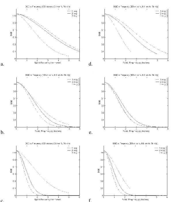
Figure 2.5: DQEeff as a function of frequency for 74 kVp. a. shows
the results for SID of 1 m and b. for SID of 2 m for 100 micron pixel and 0.1 mm focal spot. c. 100 micron pixel and d. 200 micron pixel for 0.3 mm focal spot and SID of 2 m. e. shows 100 micron pixel, 0.6 mm focal
spot and SID of 2 m. ...37
Figure 2.6: DQEeff as a function of frequency for a 100 micron
pixel, 0.3 mm focal spot, and 2 m SID. a.
mammography (28 kVp). b. general radiography (74
kVp). c. chest radiography (120 kVp). ...38
Figure 2.7: Plots of Hotelling SNR2 efficiency for a 1 mm nodule and SID of 1 m and 2 m. a. 100 micron pixel and 0.3 mm focal spot. b. 100 micron pixel and 0.6 mm focal spot. c. 200 micron pixel and 0.3 mm focal spot. d. 200
micron pixel and 0.6 mm focal spot...39
Figure 2.8: Plots of optimal magnification vs. pixel size for three focal spots and two SIDS. a. mammography (28 kVp). b. general radiography (74 kVp). d. chest radiography
(120 kVp). ...40
Figure 2.9: Plots of optimal magnification improvement (in terms of SNR2) vs. pixel size for three focal spots. a.
mammography (28 kVp). b. general radiography (74
Figure 3.1: Linearity as a function of exposure (mR) for all
exposures (a) and for lower exposures (b). ...51
Figure 3.2: Presampled spatial MTF as a function of frequency for
frame rates 100, 500, and 750. ...51
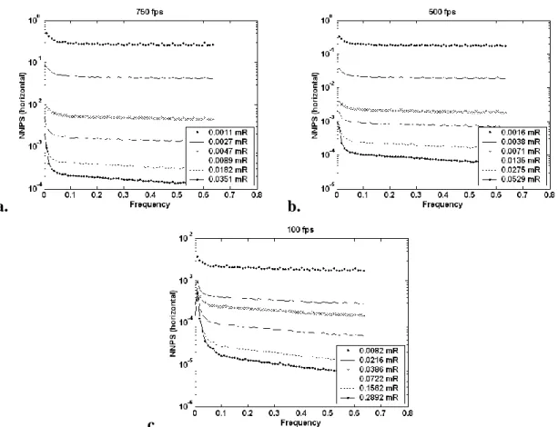
Figure 3.3: NNPSlag in units of mm2 versus frequency in units of
cycles/mm for exposures ranging from 0.001 to 0.289 mR for frame rates 750 fps (a), 500 fps (b), and 100 fps
(c). ...52
Figure 3.4: DQE versus frequency in units of cycles/mm for exposures ranging between 0.001 and 0.271 mR per frame for frame rates of 750 fps (a), 500 fps (b), and 100 fps (c). Figure d. is a plot of DQE(0) as a function
of exposure for frame rates 100, 500 and 750 fps...54
Figure 3.5: (a) Profile of the LSF generated by exposing the detector for a long duration. (b) Profile of falling LSF
determined by differentiating the extracted falling edge. ...55
Figure 3.6: The temporal MTF of falling LSF determined by using the long-exposure technique. The MTF was determined by exposing the detector with x-ray for a long duration
of time. ...55
Figure 4.1: An anthropomorphic chest phantom (left) with realistic
lung vessel structures (right). ...61
Figure 4.2: Examples of ROIs used for eNNPS calculations for single view CXR (a), stereo/BCI (b) and geometrical
phantom (c). ...66
Figure 4.3: eMTF for adult (a) and large adult (b) phantoms at two
different magnifications. ...69
Figure 4.4: CXR, stereo/BCI and geometrical phantom results for eNNPS: adult phantom at E=E0 (a), adult phantom at
E=3.2E0 (b), adult phantom 50% magnification at E=E0
(c), adult phantom 50% magnification at E=3.2E0 (d),
large adult phantom at E=E0 (e), large adult phantom at
E=3.2E0 (f), large adult phantom 50% magnification at
E=E0 (g), large adult phantom 50% magnification at
E=3.2E0 (h). ...72
Figure 4.5: CXR, stereo/BCI and geometrical phantom results for eDQE: adult phantom at E=E0 (a), adult phantom at
xiii
(c), adult phantom 50% magnification at E=3.2E0 (d),
large adult phantom at E=E0 (e), large adult phantom at
E=3.2E0 (f), large adult phantom 50% magnification at
E=E0 (g), large adult phantom 50% magnification at
E=3.2E0 (h). ...76
Figure 5.1: BCI acquisition system[22] ...84
Figure 5.2: BCI acquisition geometry where the angle α = 3o as measured from the center of the beams. ...85
Figure 5.3: Sample images (a-b) and zoom images of lesion (c-d) ...86
Figure 5.4: Stereoscopic viewing system...87
Figure 5.5: Schematic of stereoscopic image formation[94] ...88
Figure 5.6: ROC performance of PA study as dashed lines and BCI study as dotted lines for 4 radiologists (a-d). and e. Average of ROC curves ...90
Figure 6.1: BCI acquisition geometry where the angle α = 3o [15] ...97
Figure 6.2: Stereoscopic viewing system...102
ABBREVIATIONS
ALER alternate line erasure and readout
a-SE amorphous selenium
ASICs application specific integrated circuits
AUC area under the curve
BCI bi-plane correlation imaging
CAD computer aided detection
CCD charge coupled device
CdTe Cadmium Telluride
CMOS complementary metal-oxide semiconductor
CNR contrast to noise ratio
CR computed radiography
CsI cesium iodide
CT computed tomography
CXR Chest x-ray
CZT Cadmium Zinc Telluride
DCE detail contrast enhancement
xv eDQE effective DQE
eMTF effective MTF
eNNPS effective normalized NPS
ESF edge spread function
FOV field-of-view
FP false positive
FPS frames per second
GaAs Gallium Arsenide
HPM chest radiologist
IEC International Electrotechnical Commision
IRB institutional review board
LSF line spread function
MRMC multi-reader, multi-case
MTF modulation transfer function
NLST National Lung Screening Trial
NNPS normalized noise power spectrum
NPS noise power spectrum
PA posterior-anterior
PPV positive predictive value
ROC Receiver operating characteristic
ROI region of interest
Si Silicon
SID source-to-image plane distance
SNR signal-to-noise ratio
s-Si amorphous
CHAPTER 1
Introduction
The leading cause of death due to cancer in the United States is lung cancer which
results in almost one third of total deaths from cancer.[3] More women die from lung
cancer every year than breast cancer.[3] Although smoking is considered the main cause
of most lung cancer incidence, nonsmokers constitute 10-15% of lung cancer cases.[122,
138] The 5 year survival rate for lung cancer is only 16% but if detected early, the 5 year
survival rate increases to 53%.[3] Unfortunately, only 15% of cases are detected in early
stages while localized.[3] Early detection is the key to survivability. Unfortunately, for
lung cancer, there is no standard screening program like mammography for breast cancer
and therefore, most lung cancers are detected during screenings for other purposes at later
stages. A lung cancer screening program has not proven effective.[54, 91] This
dissertation examines bi-plane correlation imaging (BCI) with stereoscopic visualization
as a new modality for use in lung cancer detection. The introduction provides a
description of the challenges of imaging the chest, an overview of digital detectors and
computer aided detection as well as a summary of applications for chest imaging.
1.1 CHALLENGES OF CHEST IMAGING
Today, chest radiography is the most common method of imaging for thoracic
diseases.[76] In 2006, an estimated129 million chest radiographic procedures were
performed, more than double the second most common radiographic procedure and
almost 4 times the number of mammographic procedures.[82] Although a common
procedure, interpretation of a chest radiograph is quite difficult and has been shown to
chest anatomy, detecting subtle lung nodules with chest radiography is limited by
contrast to noise ratio (CNR), anatomical noise, and perceptual errors.[102]
Chest anatomy requires a large field of view which includes high contrast bony
structures and soft tissue structures as well as mostly transparent lung tissue. Examples
of chest radiographs can be seen in Figure 1.1. The ribs and sternum are large bony
structures surrounding the lungs which attenuate x-rays more than lung tissue. The
mediastinum is the area between the lungs which comprises the trachea, esophagus,
bronchi, lymph nodes and the heart as well as large veins and arteries of the heart. These
soft tissue structures are also much denser than lung tissue attenuating x-rays more
effectively resulting in high contrast structures. X-ray transmission through the different
structures of the thoracic cavity can vary by as much as two orders of magnitude.[76]
Visualization of low contrast features over two orders of magnitude is a challenging task.
Adequate penetration of denser structures in the thoracic cavity also necessitates larger
tube potentials which further reduce contrast.[76] The higher tube potentials necessary
together with the soft tissue structures results in Compton scattering which adds another
type of noisy background and negatively affects the image contrast especially of low
contrast features.[76] Scattering in a system without a grid can account for up to 70% of
3
a. b.
Figure 1.1 a. Posterior-Anterior chest radiograph and b. lateral chest radiograph.[53]
Chest radiography is the projection of a 3D structure onto a 2D image. Therefore,
the bony and soft tissue structures contribute to anatomic noise by potentially blocking
the view of lung nodules. Additionally, fine pulmonary vessels are numerous throughout
the lung to provide an efficient exchange of oxygen. These structures form an overall
anatomically noisy background in chest radiography. Samei and colleagues
demonstrated that anatomic noise prevents detection of subtle lung lesions more than
radiographic noise.[108, 110] For a reader to distinguish a lesion in a background of
anatomical noise, the lesion needs to be an order of magnitude larger than the same lesion
on a quantum limited background.[110] Another report determined that anatomical
obstructions result in a 71% miss rate.[130]
Perceptual errors in chest radiography result in a miss rate of 10-22%.[130]
Kundel et al classified observer perceptual errors as scanning errors, recognition errors
and decision making errors.[67] Scanning errors occur when the observer does not
lesions.[67, 76] Recognition errors occur when the observer has insufficient dwell time
in the area of the lesion and account for approximately 25% of missed lesions.[67, 76]
Decision making errors account for an estimated 45% of missed lesions, and occur when
the observer adequately dwells on the lesion but makes an incorrect decision.[67, 76]
The decision making process is hindered by the complicated anatomy of the chest.[93]
In conclusion, the chest radiograph contains several high contrast objects which
also block the lungs and are superimposed on a noisy background. The contrast to noise
ratio has been improved by the introduction of flat panel imaging systems.[35, 101, 104]
However, numerous structures in chest anatomy may prevent observers from cognitively
recognizing pulmonary lesions. If the miss rate from perceptual errors and anatomical
obstructions could be improved on the chest radiograph, lung cancer detection would be
more effective. The ability to view a chest radiograph in 3D may aid in visual
suppression of the anatomical noise.
1.2 DIGITAL DETECTOR TECHNOLOGY
In November of 1895, W. C. Roentgen discovered x-rays and two weeks later,
obtained an image of his wife’s hand.[139] For almost a century, screen-film systems
were the most common form of radiographic imaging system. In the mid 1970s, digital
radiography systems became commercially available.[99] Digital detectors have become
more prevalent in clinical practice. Improvements in memory capacity and processor
speeds of computers, as well as improvements in detector materials and smaller
electronics are some of the advances that have paved the way for digital detector
5
coupled device (CCD) or complementary metal-oxide semiconductor (CMOS) based
detectors, flat panel detectors and the emerging technology of photon counting detectors.
1.3 COMPUTED RADIOGRAPHY
The first digital radiography systems were computed radiography (CR) systems.
The first CR systems were storage phosphor systems which trap a latent image on a
photostimulable phosphor (usually BaFBr or RbBr) screen. A laser beam is used to
extract the latent image which is then detected with a photomultiplier tube (PMT) the
output of which is digitized to form the image. These systems provide a much better
dynamic range than screen-film systems while maintaining flexibility for bedside
applications and are easy to retrofit in existing screen-film systems. The screens can also
be reused for thousands of exposures unlike film. The screen depth dictates the
effectiveness of captured photons but also affects resolution. A thicker screen will have
better stopping power at the expense of decreased resolution. Further reduction in
resolution occurs because the laser beam has a spread at increased depth. Storage
phosphor CR systems lose half the stored signal because the screens emit light promptly
when exposed to radiation.[121] The laser beam activates fewer electrons at increased
depths resulting in a loss of 30% of potential signal and some of the light signal is
attenuated before reaching the surface.[120] Therefore, storage phosphor CR systems are
less efficient with lower image quality than other digital technologies[35, 99, 103] and
require a higher dose than other digital technologies.[120]
Commercial CR systems are usually composed of BaFBr or RbBr granular
phosphors but structured CsBr phosphors (similar to CsI phosphors used for indirect flat
that of flat panel detectors.[97, 120] The structure of CsBr phosphors increases the DQE
by channeling light better than granular phosphors and by allowing for a thicker phosphor
without loss of resolution.[97, 120] An initial bedside clinical study with CsBr
demonstrated improved low-contrast resolution and potential dose reduction compared to
a BaFBr system.[63]
Dual-sided CR systems are made of transparent detector material with two optical
systems to guide and collect emitted light from the front and back of the detector when
scanned by a laser beam. The detection efficiency of the system is improved since more
of the trapped electrons are released and the detector material can be thicker increasing
x-ray absorption efficiency by approximately 50% while not suffering a loss in
resolution.[24, 97] The two signals are combined resulting in over 30% improvement in
signal-to-noise ratio (SNR).[134] The DQE of the dual-sided system approached the
DQE of flat panel detector systems.[134] Dual-sided CR has been shown to improve
detection of chest lesions on a phantom better than storage phosphor CR.[134]
A new scanning technique to replace the laser scanning is line scanning CR that
simultaneously reads a row of pixels using a linear array of laser diodes.[24] The light
emission is focused and collected by optics and a linear array of CCD photosensors. This
technology provides twice the readout speed of typical laser scanning CR systems.[24]
The design is also more compact and provides better photon collection.[24, 120] A
recent study of five different CR systems concluded that a line scanning, structured
phosphor system demonstrated DQE approximately double that of traditional storage
7 1.4 CCD/CMOS DETECTORS
CCD- and CMOS-based detectors are integrated detector arrays optically coupled
to an x-ray phosphor. When the phosphor is stimulated, light is emitted that is sent to a
CCD or CMOS camera which forms a radiograph. CCD and CMOS sensors are typically
noisy due to light collection inefficiency. The detector is smaller than the phosphor
requiring the original image to be reduced in size resulting in an inefficient system since
only a small fraction of light photons are detected by the camera. The loss of light in this
manner is often referred to as a secondary quantum sink. Another disadvantage for CCD
technology is a very limited surface area due to cost, thus, CCDs cannot be used for large
area arrays which limits the field of view. Using multiple detectors improves the
efficiency but increases the cost and requires stitching smaller images together to form
the full image. CMOS technology provides pixel level electronics that improve the
financial restrictions of a large area array. However, excessive noise and high dark
current remain issues. Thick housing necessary to accommodate the electronics makes
retrofitting difficult.[141] The DQE of CCD/CMOS detectors has been shown to be
lower than that of flat panel detectors.[116] Due to the size limitations, most
CCD/CMOS detectors have been used for mammographic and dental applications except
for slot-scanning applications for chest (discussed later in this introduction).
1.5 FLAT PANEL DETECTORS
Imaging modalities such as bi-plane correlation imaging are feasible with the use
of flat panel detectors because of the large field-of-view (FOV), fast acquisition and
other digital technologies,[35, 84] to have better contrast to noise ratio[35, 101, 104] and
provide the ability to acquire digital images quickly.
Flat panel detectors are direct or indirect in design. Direct designs use a
photoconductive layer of amorphous selenium (a-Se) that converts x-ray energy to an
electronic charge. The electronic charge is then guided by an electric field to a storage
capacitor. Indirect designs use a phosphor layer which can be made of a GadOx
(Gd2O2S) screen or cesium iodide (CsI) that converts x-ray photons to visible light
photons that is then converted to a charge by a photodiode. The charge is then stored in a
capacitor until readout. CsI is a structured phosphor which produces better conversion
leading to improved DQE and lower dose; as such, CsI is typically used in medical
applications.[101] Both approaches use amorphous silicon (a-Si) array technology found
in laptops. The individual pixels comprise a storage element and a switching element.
The sensing element has an associated fill factor which depends on the size of the pixel.
The switching device used is typically a thin-film transistor (TFT).
The concept of the image pixel is simple: the pixel is charged by the x-ray
photons incident and then read accordingly when the switching device is activated.
However, design of the pixel results in various tradeoffs. Not only are there cost
consequences for fabrication when designing smaller pixels, but the amount of charge
that can be detected is also affected, particularly for indirect designs. For direct designs,
the electric field shaping within the photoconductor guides the charge to individual pixels
allowing the entire a-Se surface to be available for x-ray conversion.[23, 141] This type
of conversion process results in efficient pixels with fill factors approaching 100%.[23]
9
improves the resolution of the panel but is more costly to fabricate and less efficient since
fewer photons will be detected.
The a-Si array is a 2D rectangular array comprised of pixels where each row of
pixels is connected to the same horizontal control line and each column of pixels is
connected to the same vertical data line. Once an x-ray exposure is made, the
information in the storage elements is read one line at a time such that all the pixels in
that row are connected to their corresponding data line. With TFT switches, the readout
of the capacitor resets the pixel preparing it for the next charge. The readout proceeds
line by line and takes approximately 30-50 msec to complete readout of the full array.
A-Si technology suffers from charge carryover or ghosting effects due to charge trapping in
the a-Si elements[16, 128] and sensitivity variations in the photoconductor or
phosphor.[141] Once the array is read, the signal is amplified by application specific
integrated circuits (ASICs) tailored to the specific characteristics of the a-Si array. The
noise components of the ASICs must be closely monitored. After the signal is amplified,
it is digitized and stored. To maintain a compact profile, the electronics are typically
folded beneath the array using a flexible tab package. However, the compact design also
leads to thermal drift issues requiring frequent dark current calibrations.
Direct detectors exhibit nearly perfect modulation transfer function (MTF) since
there is no phosphor for light spread. The MTF of indirect detectors is comparable to that
of CR systems. The noise power spectrum (NPS) of direct detectors is similar to white
noise. The light spread in indirect detectors generally improves the NPS by introducing
blur into the system, thus noise is reduced compared to direct detectors. The absorption
but the almost ideal MTF of the direct system results in a better DQE for higher
frequencies. This indicates there is a task dependent tradeoff such that direct detectors
may exhibit improved performance for high detail and high contrast structures and
indirect may have improved performance for low contrast objects in noisy backgrounds
like chest radiography.[105] Bacher, et al confirmed this result in an observer study to
compare direct and indirect flat panel detector systems when detecting subtle lung
nodules.[7] A recent study for chest radiography showed that a reduced dose could be
used with an indirect system that achieved equal or superior performance compared to a
direct system.[7]
The DQE of flat panel detectors has been found to be better than that of CR
systems.[104] Due to the various stages of signal loss in CR systems compared to
indirect flat panel detector systems, this result is not unexpected. One study concluded
that an indirect flat panel detector could be operated at exposure levels 3.7 times lower
than a comparable CR system.[104] Flat panel detectors have inherent dark current noise
that CR systems do not possess.[99] Currently, flat panel detectors are more expensive
than CR systems but work is being done to reduce the cost while flat panel detector
technology continues to improve. Advances under investigation to improve the gain and
thus the SNR include replacing discrete photodiodes in indirect designs with a continuous
photodiode to increase the pixel fill factor, using amplifier circuits in the pixel for direct
or indirect designs and incorporating photoconductive materials with higher signal
11
1.6 PHOTON COUNTING DETECTORS
A promising technology beginning to attract more attention in digital radiography
is photon counting detectors. X-ray sources used in medical imaging produce
bremsstrahlung radiation which has a broad energy spectrum. Previous detectors
discussed based on phosphor technology are integrating systems which integrate all
energies into a single energy bin. With photon counting detectors, x-ray energy
discrimination can be performed such that the low energies enhance the softer tissues
while high energies enhance harder tissue like bone. Photon counting detectors possess
low noise, linearity and infinite dynamic range[36, 123] while providing the ability to
reject scatter, improve SNR and decrease dose.[98] Compositions of GaAs (Gallium
Arsenide), Si (Silicon), CdTe (Cadmium Telluride), and CZT (Cadmium Zinc Telluride)
as well as others under investigation have been used for photon counting detectors.[98]
Several issues with this technology need to be resolved such as energy window
optimization or resolution, spatial resolution, choice of detector material, and fabrication
complications.[36, 98, 123] Narrow energy window selections will result in quantum
limited noise while wider energy windows will result in less energy discrimination or
resolution. Spatial resolution depends on the pixel size but is also affected by blurring
due to charge sharing between pixels.[123, 126] Charge sharing depends upon the
thickness of the material and the applied electric field.[126] Detector materials used need
to have good absorption of incident photons and be resilient when exposed to high
temperatures and shearing while maintaining minimum leakage which allows for more of
challenging task but as electronic circuits continue to be improved, fabrication should
become more feasible with minimal spacing between pixels for lower cost.
1.7 COMPUTER AIDED DETECTION
Approximately 30% of lung nodules are not detected during a first reading but
can be detected when viewed retrospectively.[66, 85] As previously discussed,
perceptual errors by the observer result in a high miss rate and observers are known to
have subjective and inconsistent decision criteria.[44] Due to time and cost constraints,
having an observer perform a second reading is not always practical; therefore, computer
aided detection (CAD) can be used as a second reader by directing the attention of the
observer to suspect nodules. CAD involves the segmentation, extraction and
identification of potential pulmonary nodule candidates. CAD algorithms start with
image enhancement in the form of histogram equalization and filtering. As stated
previously, the biggest hurdle to lung nodule detection is overlapping anatomy in chest
radiography. Therefore, the first step after initial image enhancement in CAD routines is
the suppression of overlying anatomy typically by means of image subtraction techniques
that attempt to remove normal structures like ribs and soft tissue. Lung field
segmentation using rule-based reasoning or pixel classification is performed to limit the
search area.[45] Initial nodule candidates are then determined by various methods
including filtering and unsharp masking to enhance the nodules and then template
matching or Hough transforms to detect candidates. Specific nodule features such as
radius, circularity, diameter, curvature, ellipticity and contrast are then used to minimize
the set of false positives. The final detected set of nodules is presented to the observer to
13
positives accurately is a difficult task. Using data from multiprojection images to
correlate the CAD findings could result in further reductions of false positives.[102, 117]
Limited commercial options for chest CAD (Edda Techonology and Riverain
Technologies) currently exist, but CAD could become a useful tool in clinical settings as
techniques/algorithms continue to evolve. CAD as a second reader with a commercially
available system has been shown to improve the detection of lung nodules with chest
radiography and to be more effective for less experienced radiologists.[61, 70] Work still
remains to test the clinical effectiveness of CAD on large data sets.
1.8 APPLICATIONS FOR CHEST IMAGING
Recently, the National Lung Screening Trial (NLST) has shown a 20 percent
decrease in death due to lung cancer.[60] The NLST used computed tomography (CT) as
the image screening tool. CT limits anatomical obstructions compared to chest
radiography; however, in comparison, CT requires a much higher radiation dose. One
study reported that the average effective dose from a chest posterior-anterior (PA) exam
is 0.039 mSv while the average effective dose of a chest CT exam is 3.2 mSv.[142] The
number of CT exams has increased rapidly in the last decade and CT is one of the largest
sources of radiation exposure from medical imaging.[12, 18, 32, 51, 81] One study
reported that CT and nuclear imaging procedures were performed on 21% of the study
population but the exposure was 75.4% of total effective dose.[32] In contrast, 71.4% of
the population received radiography exams which comprised only 10.6% of the total
effective dose.[32] Dose reduction strategies for CT are being pursued;[77] however, CT
exams are a larger financial burden that require more extensive postprocessing techniques
tool, a low dose, low cost option would also be beneficial. Lower dose applications
currently available that minimize anatomical structure noise are dual-energy[5, 69, 100]
and tomosynthesis[28, 29, 136]. Slot-scanning systems have also demonstrated improved
detection of subtle lung nodules through reduced scatter. Bi-plane correlation imaging is
a recently proposed application for detecting subtle lung nodules.
1.9 SLOT-SCANNING SYSTEMS
Slot-scanning systems incorporate a moving CCD based detector synchronized
with a moving beam source that is collimated to produce a narrow fan beam. The
collimated beam eliminates the need for an anti-scatter grid while providing better scatter
rejection than full field applications with anti-scatter grids. One study of a slot-scan
system for chest reported scatter fraction reductions of 22-25% in the lung and 16-18% in
the denser regions with an anti-scatter grid while the slot-scan system at the same tube
potential demonstrated scatter fraction reductions of 54% and 47-57% respectively, a
significant improvement.[111] In the same study, the PA dose from the slot-scan system
was 16% higher than the full field chest system. Although the flat panel detector in the
full field chest system has a higher DQE, the reduction of scatter in the slot-scan CCD
system resulted in an improved SNR.[111, 116, 120] Slot-scan systems using CCDs
require careful alignment and synchronization between the CCD detector and the fan
beam.[72, 73] Slot-scanning systems have inefficient tube usage and the total imaging
time is 1.3 seconds compared to 20 msec for standard PA studies[116]. Recent studies
have investigated using flat panel detectors in slot-scan systems. The readout electronics
of the flat panel detector are modified using an alternate line erasure and readout (ALER)
15
instead of line by line.[72, 73] The leading edge line is reset to erase the scatter
component while the trailing edge is read to acquire the exposed image.[72, 73] Using
this method with an 18 mm slot width, the scatter was reduced by over 86%.[72]
Improved scatter rejection results in better image contrast.[72] As Liu, et al emphasizes,
the scatter reduction is dependent on the slot width which is more easily altered with
digital collimation. One concern with the ALER technique is adequate erasure of the
scattered radiation but Liu, et al demonstrated that erasure is successful. A slot-scan
system takes longer to acquire the image but only a small portion of the image is being
acquired at any given time therefore, patient motion is not a significant factor.[72, 116]
With slot-scan systems, there is a tradeoff between tube loading and slot width. A wider
slot-width decreases the necessary tube loading at the expense of increased scatter.[72]
Determining optimal imaging parameters remains an issue with slot-scan systems.
1.10 DUAL-ENERGY SYSTEMS
Dual-energy systems require a double exposure with different dose techniques
which are then subtracted to remove anatomical structures, particularly bone and soft
tissue. Dual-energy with CR systems allows the low and high energy images to be
recorded concurrently with a single exposure. The CR system is composed of a copper
filter between two plates. The first plate records a typical PA chest image, and then the
copper filter hardens the beam such that the second plate records the higher energy beam.
Since the two images are taken in one exposure, there is no time delay and therefore, no
patient motion so the two images can be subtracted cleanly. Dual-energy with flat panel
detectors requires two exposures in which, although only separated by milliseconds,
post-processing for noise reduction and image registration.[96, 100] When the two
images are subtracted, edge artifacts typically exist in the bone and tissue images.[5, 34,
76] The flat panel detector dual-energy systems have better energy discrimination and
lower noise due to better image quality than the CR systems[5] but are higher dose.
Recent studies of dual-energy systems in conjunction with PA chest radiographs
demonstrated improved detection, but the value of the modality for lung nodule detection
and type of imaging parameters employed are still under discussion.[69, 100] Flat panel
detector systems also provide the ability for dynamic dual-energy studies. Recent
advances demonstrated feasibility of dynamic dual-energy flat panel detector systems for
use in functional lung imaging and tumor motion.[140] Photon counting detectors
composed of CdTe recently developed for use in a dual-energy application demonstrated
count rates and noise limits suitable for use in dual-energy radiography applications.[8]
1.11 TOMOSYNTHESIS SYSTEMS
Tomosynthesis is a form of limited angle tomography that provides a reduction in
anatomical noise similar to CT at a much lower dose and cost.[28, 136] Tomosynthesis
systems incorporate a conventional x-ray tube source, digital detector and a custom tube
mover allowing for easy implementation. Most tomosynthesis images are acquired in the
conventional PA projection. The high DQE and scanning rate of flat panel detectors have
made tomosynthesis practical for clinical use. Imaging time for tomosynthesis is
typically one breath hold or about 10-11s and the dose is comparable to conventional
chest radiography.[29] Similar to CT, projection images are acquired as the x-ray tube
moves, for tomosynthesis, movement occurs along a vertical path. The projection images
17
simple shift and add equivalent to simple backprojection.[29] Changing the shift
parameter generates slices throughout the entire volume bringing different planes into
focus. The shift and add technique is simple, but results in blur that must be minimized
through various deblurring techniques including matrix inversion, filtered backprojection
and iterative restoration.[29] Although tomosynthesis does not provide the depth
resolution of CT, the performance is superior to conventional chest radiography. Recent
clinical studies demonstrated improved detection of lung nodules using tomosynthesis
compared to chest radiography.[26, 136] Tomosynthesis reconstructions may contain
artifacts from the limited angle acquisition and further analysis needs to be performed to
ascertain clinical effectiveness in detection of pulmonary nodules.[28, 29, 136]
1.12 BI-PLANE CORRELATION SYSTEMS
A low dose, low cost, fast acquisition modality that may provide a feasible
alternative for lung cancer screening without post-processing algorithms is bi-plane
correlation imaging (BCI) with stereoscopic display. The use of stereo/BCI has become
feasible with flat panel detector systems which provide fast acquisitions necessary for
minimal motion artifacts resulting in successful correlation without the use of registration
algorithms. Viewing bi-plane correlation images in 3D on a stereographic display will
suppress anatomical obstructions. Studies for stereomammography have shown that
stereo/BCI of the breast is feasible.[42, 43, 119] Preliminary studies of BCI for chest
using phantoms and a small patient subset demonstrated that chest BCI is feasible.[102,
117] The preliminary studies also explored the use of computer-aided detection (CAD)
with the correlated images.[88, 89, 102, 117] CAD algorithms as second readers in chest
result in high false positive findings.[13, 61] The angular images from BCI provide
correlated data to use in CAD algorithms which improve the false positive rate. 5,25
Viewing the bi-plane images stereoscopically provides the radiologist with a
visual reduction of anatomical noise. Stereoscopic photography was popular at the turn
of the twentieth century and physicians at that time developed techniques for viewing
medical images stereoscopically.[42] Viewing the x-ray films required awkward
handheld viewing devices and involved difficult alignment of the images.[42] However,
stereoscopic imaging was used in radiology departments until CT and MRI systems
became available.[42] Stereoscopic vision occurs because the human eyes are
approximately 65 mm apart causing horizontal parallax so that the left eye and right eye
receive slightly different views resulting in a horizontal angular disparity of points in the
retinal images from each eye. Within the visual cortex, these two views are fused into a
single view with depth perception. Stereoscopic monitors are designed to display the left
image only to the left eye and the right image only to the right eye. Two types of
monitors exist for viewing images stereoscopically. Autostereoscopic monitors do not
require the use of special glasses or headgear while stereoscopic monitors do require the
use of special equipment.
Autostereoscopic monitors use parallax barriers or lenticular lenses. Parallax
barriers interleave the left and right eye images on the display. Early systems did this
with various types of grid plates that provided vertical strips alternating the left and right
images but recent technology uses tiny lenses integrated into the layered liquid crystal
displays. Each layer contains small stripes that hide specific pixels such that some are
19
to remain in a fixed location. Lenticular lens sheets contain lenses that refract left and
right images. Recent advances in 3D monitor technology have multiple lenticular lenses
at different angles so the observer does not need to remain in a fixed position since the
image received depends on the viewing angle.
Stereoscopic displays that require special viewing equipment simultaneously
provide left and right images through separate channels and are said to be spatially
multiplexed.[42] Analog methods of separating the channels either split the screen into
left and right images or uses two monitors to display the left and right images. Then a
device with mirrors and optics is attached to the system to deliver the appropriate image
to the appropriate eye. The images can be displayed on a single monitor using temporal
multiplexing where the left and right images are alternately displayed. These systems
require optical shutters in the eyewear to insure that the left image is only shown to the
left eye and the right image is only shown to the right eye and the shutters in the eyewear
have to be synchronized to the display and require a high refresh rate to avoid flicker.
1.13 OBJECTIVES AND ORGANIZATION
This study explores the feasibility of stereo/BCI systems for detecting subtle lung
nodules in human subjects by optimizing system geometry, investigating the effective
DQE (eDQE) of a clinical imaging system, characterizing flat panel detectors and
stereoscopically viewing bi-plane images in observer studies. The work was undertaken
to assess the effectiveness of BCI viewed stereoscopically for detection of lung nodules.
The first part of the study involved a theoretical assessment of system geometry
for standard PA chest exams and extension of the DQE to analyze the effective DQE
commercially available CsI flat panel detector was also performed. Initial introduction of
flat panel detectors resulted in a simple substitution of the flat panel detector for the
analog screen film or CR cassette. Studies have since shown that flat panel detectors
improve DQE such that dose can be reduced compared to screen film and CR.[33, 35]
However, the optimal system geometry of flat panel detectors has not been sufficiently
evaluated. In Chapter Two a theoretical framework was established to assess the tradeoff
of different geometries for standard PA acquisitions. The flat panel detector used for the
prototype bi-plane correlation system was characterized for image quality in Chapter
Three. DQE has been the standard metric used to describe system performance;
however, DQE is a detector specific metric.[112] The eDQE has been investigated as a
metric to more accurately describe overall system performance.[113] Chapter Four
examines the eDQE of a clinical system used for chest radiography.
For the second part, observer studies were performed on bi-plane human subject
data viewed stereoscopically. The BCI system acquired a PA image as well as images at
oblique angles or ± 3 degrees of PA in the horizontal direction as determined in previous
studies.[88, 89, 102, 117] Chapter Five reports the preliminary results of the observer
study. After the preliminary study, simulated lesions were added to the normal cases and
the order of viewing the images was modified for a second observer study. In addition, a
correlated CAD algorithm was used to act as a second reader during the second observer
CHAPTER 2
Imaging properties of digital magnification radiography 2.1 INTRODUCTION
Flat panel detectors are becoming increasingly prevalent in the imaging market
for many applications including those in medicine, veterinary medicine, and
manufacturing. Studies are being performed to use these devices in all areas of clinical
radiology including diagnostic radiography, fluoroscopy, and mammography, as well as
research areas of tomosynthesis and cone beam computed tomography (CT).[78, 79] In
most situations, flat panel detectors have simply replaced the current receptor in a system
without changing other parameters of the acquisition such as the geometry. Several
studies have been performed to show that flat panel detectors offer improved SNR over
competing technologies.[6, 21, 38, 49, 127] However, some studies have suggested
potential benefits of magnification for various radiology examinations using film or flat
panel detectors.[14, 86, 124, 129, 132] In particular, standard clinical practice is to use
magnification mammography with film-screen systems for diagnostic follow-up to
screening mammography.[25, 52, 68, 75, 92] To date, clinical applications have not
taken advantage of the improvements offered by magnification.
The goal of the current work was to examine the effects of geometry by studying
the impact of magnification on image quality in radiographic imaging. A theoretical
model was developed to investigate how the geometry of image acquisition with a flat
panel detector can be optimized in terms of various acquisition parameters such as focal
____________________
This chapter is based on a paper by Sarah J. Boyce and Ehsan Samei published in Medical Physics 2006.
spot size, pixel size, SID (source-to-image plane distance), and air gap. The image
quality for optimization was assessed using standard metrics, MTF, NPS, DQE, and
effective DQE (eDQE).[111, 116] Furthermore, the framework was applied to three
specific imaging applications, mammography, general radiography (also applicable to
mammotomography[79]), and chest radiography, to investigate how these applications
can be optimized from a geometrical perspective.
2.2 METHODS
This work uses the traditional cascaded system model of
source-object-detector-observer to study optimum geometry. Optimum geometry is determined by examining
image acquisition parameters that affect system performance in terms of resolution,
noise, SNR, and SNR in the presence of scattered radiation. Traditional image quality
parameters such as MTF for resolution, NPS for noise characterization, DQE for SNR,
and effective DQE for overall SNR are examined in terms of tradeoffs between image
acquisition parameters such as focal spot size, SID, air gap, and pixel size. These image
quality parameters are adequately described in Fourier space if the system is assumed to
be shift invariant and linear.[127] When possible, these metrics are reduced to scalar
figures of merit to characterize the overall system performance.
All image quality characteristics are determined in the frequency domain of the
object plane denoted by primes with u’ representing the frequency in the object plane and
u representing the frequency in the image plane. Thus, if the resolution limit (i.e., the
cutoff frequency or highest spatial frequency which can be reliably reproduced) is
23
where m is the magnification factor. For simplicity, all model calculations are performed
for a single dimension and assumptions made for calculations are equally applicable to
the two dimensional case. The linearized-single dimension treatment provides a
reasonable approximation for inherent response of a digital radiographic system, as long
as the approximation does not extend to spatial frequencies close to the Nyquist
frequency where the system response becomes non-stationary, violating one of the
requirements of the linear system analysis.
2.2.1 Modulation Transfer Function Model
The modulation transfer function (MTF) as a function of the amplitude of the
Fourier transform of the point spread function versus spatial frequency is the most
common metric to characterize the spatial resolution of an imaging system.[90, 103, 104,
118] The MTF is often characterized in the image plane. In the object plane, the system
MTF, MTF(u’) = MTF(u/m), represents the MTF in the image plane scaled by
magnification.
In Fourier space, the total MTF for the system results from multiplying the MTFs
of the individual system components. Our model includes the resolution of two
components, the detector MTF and the focal spot MTF.
The MTF for the detector is derived in the object plane by treating the pixel and
the phosphor as two separate elements of the detector. The theoretical phosphor MTF
where u’ is the spatial frequency in the object plane, assumes the form
o phos u u' αln erfc 2 1 (u' M TF
based on the Burgess model for phosphors which has been shown to correspond well with
empirical data.[19, 103] For this model, α is the slope and u0 is the frequency where the
MTF is 0.5. The pixel MTF is modeled as a sinc function,
u' w ) u' sin(w (u' M TF pix pix
pix
, (2.2)
where wpix is the pixel width assuming square pixels. The total detector MTF which
combines Eqs. (2.1) and (2.2) is then
MTF (u' MTF (u'
(u'
MTFpanel pix phos
. (2.3)
Although the source distribution may be complex,[9] the MTF associated with the focal
spot blur may be reasonably modeled using a Gaussian distribution as in previous work
by Siewerdsen and Shaw[124, 129]
2 ' w m 1 -m -fs fs e M TF
u , (2.4)
where wfs is the full width at half maximum (FWHM) of the focal spot and m is the
magnification. The presampled system MTF in the object plane can therefore be
represented as
MTF (u' MTF (u'
MTF(u' panel fs
. (2.5)
Geometric sharpness[129] provides a scalar figure of merit for characterizing the overall
resolution across the frequency range. The geometric sharpness can be defined as the
integral of the square of the MTF[129]
N
f
0 2
geo M TF (u')du'
s
, (2.6)
25 2.2.2 Noise Power Spectrum Model
A quantitative representation of the noise properties of flat panel detectors is
commonly provided by the noise power spectrum (NPS) which can by thought of as the
variance of image noise across various frequencies.[41, 103, 104, 135] In this work, the
theoretical model for the presampled NPS (NPSpre(u)) is based on the assumption that the
correlated noise component is proportional to the receptor MTF2 for a deterministic
spreading stage which generalizes the model described by Siewerdsen[127] for a
cascaded, linear flat panel detector. Thus
additive 2
panel(u NPS
MTF * η
NPS(u , (2.7)
where η is the scale factor accounting for specific receptor properties,[127] NPSadditive
represents the additive noise component from the gain stage of the digital detector and is
assumed to have a scalar value, and MTF2panel is the panel MTF obtained by aliasing the
presampled MTF as,
) u' (2f MTF ) (u' MTF ) (u'
MTFsam pre pre
, (2.8)
where f is half the sampling rate. The normalized sampled NPS (NNPS(u’)) is then
obtained by performing a non-linear fit of the model in Eq. (2.7) to experimental data
from a previous study.[103, 135]
The model provides the NPS in the image plane, NPS(u). Since NPS is a function
of area, the effect of magnification must be considered to account for the difference
between the pixel size in the image plane and the effective pixel size in the object plane,
thus
NPS(u/m) m
1 ) NPS(u' 2
represents the NPS in the object plane.[111, 116, 124]
2.2.3 Scatter Rejection Model
Compton scatter is the primary source of scattered photons associated with x-ray
imaging and if detected, leads to a loss of contrast and added noise.[129] Increasing the
object-image distance not only increases magnification, but also reduces scatter. Air gaps
and grids are often used to reduce scatter. In this work, only the air gap technique is
considered as it provides equivalent or even potentially superior scatter rejection
performance compared to grids without any loss of primary radiation associated with
grids.[64, 111]
The effects of scatter on the geometry are described using the effective scatter
point source (ESPS) model first developed by Muntz et al.[87] Muntz et al. described
scatter rejection from an air gap by defining an effective scatter point source located
between the source and the exit surface of the object. In this model, the
scatter-to-primary ratio at the image plane (SP) can be calculated as
SF 1 SF m x x SP SP 2 2 s s o
g , (2.10)
where xs is the distance between the effective scatter source and the object exit plane, SPo
is the scatter-to-primary ratio at the object plane, g is the air gap distance, m is the
magnification, and SF is the scatter fraction. Our model was modified such that the
effective scatter point source is located between the source and the center of the object.
2.2.4 Detective Quantum Efficiency Model
The DQE is commonly used as an image quality metric for signal to noise
27
is calculated in the object plane with the system MTF from Eq. (2.5) and the sampled
NNPS as described in section II. B. as
) NNPS(u' qEm ) (u' M TF ) DQE(u' 2 2
, (2.11)
where q is the square of the ideal signal-to-noise ratio (SNR2) per exposure with units of
mm-2-mR-1 and E is the exposure in units of mR. The m2 factor accounts for the change
in exposure as a function of magnification and cancels the 1/m2 factor inherent in the
NNPS(u’), Eq. (2.9).
This model does not account for x-ray scatter effects that introduce extra noise
into the image. To describe this effect, the effective DQE as proposed by Samei et.
al.[111, 116] is used,
) SF)DQE(u' t(1
)
eDQE(u' , (2.12)
where t is the transmission of primary x-rays through the extra detector elements prior to
reaching the detector, and SF is the scatter fraction that reaches the detector [where SF =
SP/(SP + 1)].
2.2.5 Observer Model
While DQE and eDQE provide generic descriptions of SNR, they do not reflect
the effects of a specific signal on object detectability. This can be achieved using the
Hotelling SNR2 which includes a signal term.[107] The Hotelling SNR2 efficiency is the
Hotelling SNR2 per unit exposure defined as
du' )u' eDQE(u' ) (u' S 2π F N f 0 2
where eDQE(u’) is the effective DQE as defined by Eq. (2.12), and S(u’) is the Fourier
transform of the nodule model.
The nodule was modeled using the designer profile defined by Samei and
Burgess[20, 107] calculated using the Hankel transform
1 n 1
n
designer(u') J (2 Ru')/(2 Ru')
S , (2.14)
where Jn+1(2πRu’) is a first order Bessel function, R is the diameter of the nodule, and n
is an exponent defining the shape of the nodule. Values of n between 1 and 2 represent
reasonable lesion approximation.
2.2.6 Model Input Parameters
Pixel sizes were varied within a 50-200 micron range. For each pixel size, the
nominal focal spot sizes of 0.1, 0.3, and 0.6 mm were used. For each combination of
pixel size and focal spot size, magnification values from 1 to 3 were considered. The
initial MTF and NNPS experimental data were obtained at 28 kVp with exposure of 32.8
mR and a q of 53300 photons/mm2-mR,[135] 74 kVp with exposure of 0.27 mR and a q
of 255855 photons/mm2-mR,[103] and 120 kVp with exposure of 0.24 mR and a q of
259231 photons/mm2-mR.[104] The MTF data were fitted to the Burgess model of Eq.
(2.1) which was then assumed to have fixed α and u0 values for model MTF calculations
associated with each technique. The NNPS data were used to perform a nonlinear fit to
the generic model in Eq. (2.7) which was then assumed to have fixed η and NPSadditive
components. These assumptions were made as the thickness of the phosphor was not
considered as a variable parameter in the model. Table 2.1 summarizes the input
29
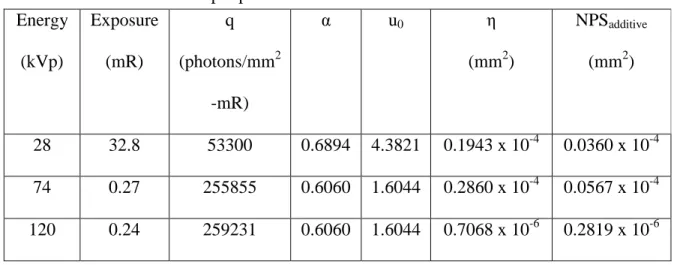
Table 2.1: Input parameters for MTF and NNPS calculations Energy
(kVp)
Exposure
(mR)
q
(photons/mm2
-mR)
α u0 η
(mm2)
NPSadditive
(mm2)
28 32.8 53300 0.6894 4.3821 0.1943 x 10⁻⁴ 0.0360 x 10⁻⁴
74 0.27 255855 0.6060 1.6044 0.2860 x 10⁻⁴ 0.0567 x 10⁻⁴
120 0.24 259231 0.6060 1.6044 0.7068 x 10⁻⁶ 0.2819 x 10⁻⁶
Table 2.2 summarizes input parameters for scatter calculations. The desired field
size used was 120 cm2. The tissue thickness (assumed uniform), xs, and SP0 values for
28 kVp were obtained from work done by Krol et. al.[64] while those for 74 kVp and 120
kVp were derived using a linear fit to data from Sorensen and Floch.[132] The SID was
assumed fixed and the air gap distance was varied by moving the object. Two values for
SID were used, 1 m and 2 m. The designer nodule was used with a diameter of 1 mm and
Table 2.2: Input parameters for scatter calculations Application Energy
(kVp)
Tissue
Thickness
(cm)
xs (cm) SP0
Mammography 28 6.2 16 1.00
General
Radiography
74 8 15.78 2.01
Chest
Radiography
120 8 13.79 2.32
2.3 RESULTS
From the multiple combinatorial set of model results for all the influencing
parameters, the following results considered the effects of each of the factors, focal spot
size, pixel size, scatter fraction, and SID, on magnification and the corresponding effects
on the MTF, NPS, and DQE.
2.3.1 Effects of Magnification on MTF
The focal spot MTF degraded with magnification while the detector MTF
improved with magnification. Representative results shown in Figure 2.1 demonstrate
that the improvement of the MTF depended on the tradeoff between focal spot size and
pixel size. A large focal spot (0.6 mm) resulted in little or no resolution improvement
with the use of geometric magnification. Since the focal spot blur dominated the system
sharpness, reducing the effective pixel size did not compensate for the loss of resolution.
31
improvement in resolution for lower frequencies but not for higher frequencies
suggesting a task dependent tradeoff for this combination (i.e., depending on the
characteristics of the features that need to be imaged, different parameters may be
optimal). A 0.3 mm focal spot with a 200 micron pixel size showed an improved MTF
for all magnification values although there was an optimum magnification. Magnification
with a 0.1 mm focal spot resulted in improved MTF out to very high frequencies
regardless of pixel size; specifically for large pixel sizes as the resolution of systems with
large pixel sizes and small focal spots were dominated by the pixel size. Magnification in
such systems resulted in a smaller effective pixel size thus increasing the overall system
resolution.
a. b.
c. d.
The geometric sharpness was used as an overall figure of merit for spatial
resolution averaging across frequencies. Figure 2.2 provides a composite graphic for
identifying the optimum magnification as a tradeoff between pixel size and focal spot
size. Note the shape of the curves differ for each focal spot size indicating that the
maximum benefit from magnification varies as a function of focal spot and pixel size. If
focal spot blur does not dominate the spatial resolution (0.1 mm focal spot),
magnification provides improvement for all pixel sizes. As focal spot blur begins to
dominate spatial resolution (0.3 mm focal spot), the improvement from magnification
reaches a maximum in the range of 1.3-1.5. For 0.6 mm focal spot, the focal spot blur
dominates the spatial resolution of the system such that magnification provides minimal
33
a. b.
c. d.
Figure 2.2: Geometric sharpness as a function of magnification for three focal spot widths and four pixel sizes.
As an implicit assumption of this study, the MTF did not change with beam
quality and thus the results shown are representative of all the radiographic imaging
applications considered in this study.
2.3.2 Effects of Magnification on NPS
Figure 2.3 shows that NNPS decreased with increased magnification for lower
frequencies primarily due to the 1/m2 factor used to estimate the NNPS in the object
plane. The magnification factor can be seen on the y-axis in the difference of the
a. b.
c. d.
Figure 2.3: Semilog plot of NNPS as a function of frequency for three magnifications and four pixel sizes for 74 kVp.
Magnification also increases the cutoff frequency as shown in Figure 2.3. Notice
the aliasing at higher frequencies, evident by the curves beginning to curve upwards in
the vicinity of the cutoff frequency. Furthermore, for smaller pixel sizes, the NNPS is
higher at higher frequencies. This effect is a result of magnification. Since magnification
decreases effective pixel size in the object plane, the frequency shift parallels an
improvement in resolution. Improved spatial resolution means less blurring which results
in increased noise.
The results shown in Figure 2.3 at 74 kVp are representative of NNPS figures at
35 2.3.3 Effects of Magnification on DQE
Figure 2.4 reports the effects of geometric magnification on the DQE for the
combinations of parameters previously defined. Results match experimental results of
Samei et. al. For small focal spot sizes (0.1 mm), magnification improves the DQE
across all frequencies. A noticeable improvement occurs at higher frequencies since
magnification shifts the cutoff frequency. For mid-range focal spot sizes (0.3 mm), the
effect of magnification is varied. Magnification improves the DQE for larger pixel sizes
(150 and 200 microns) but only marginally at lower frequencies for smaller pixel sizes
(50 and 100 microns). Also of note is that a crossover point occurs for 0.3 mm focal spot
size. For large focal spot sizes (0.6 mm), magnification provides no improvement in the
a. d.
b. e.
c. f.
Figure 2.4: Plots of the DQE as a function of frequency for 74 kVp, three magnifications and two pixel sizes, 100 micron (a., b., c.) and 200 micron (d., e., f.).
Figure 2.5 shows the eDQEresults. Since the eDQE accounts for scatter in the
system, the eDQE values are lower than the DQE values. Magnification and larger SID
37
scatter. The scatter reduction and thus the eDQE improves for the same magnification
when a larger SID is used. The magnification shows an optimum value around 1.5.
a. b.
c. d.
e.
Figure 2.5: DQEeff as a function of frequency for 74 kVp. a. shows the results for SID of
![Figure 1.1 a. Posterior-Anterior chest radiograph and b. lateral chest radiograph.[53]](https://thumb-us.123doks.com/thumbv2/123dok_us/8110634.2150733/19.918.147.764.120.410/figure-posterior-anterior-chest-radiograph-lateral-chest-radiograph.webp)