The aim of this paper is to highlight problems encountered in the factor analysis of items and to demonstrate two ways in which these problems may be dealt with, namely item response theory and item parcelling. Factor analysis is an analytic technique used to identify a reduced set of latent variables, called factors, which explain or account for the covariances of a larger set of related observed variables. In unrestricted or exploratory factor analysis, the aim is to establish the minimum number of latent variables that can adequately explain the covariances among the observed variables.
In an unrestricted factor analysis the meaning of a latent variable is typically determined by inspecting the content of the observed variables that have strong relations with it. For instance, if a factor has strong relations with observed variables that reflect the ability to solve verbal problems, one may conclude that the factor represents verbal ability. In restricted or confirmatory factor analysis, however, the researcher has an explicit hypothesis regarding the number of latent variables, the meaning of the latent variables, and how they relate to the observed variables. The aim of confirmatory factor analysis is to examine how well the hypothesised factor structure accounts for the covariances among the observed variables.
Within the context of psychological test construction, individual items typically represent the observed variables, and the constructs that the test or scale is supposed to measure represent the latent variables or factors. By subjecting items to an unrestricted factor analysis, test constructors hope to discover a smaller number of psychologically meaningful factors that account for the covariances among the items. Clusters of items with strong relations with a factor are typically combined to form a scale.
Very often, however, test constructors have explicit hypotheses regarding the way items should combine to form scales. Confirmatory factor analysis may be used to test the validity of
these hypotheses. Here the items serve as observable indicators of the latent constructs that directly correspond to the traits or characteristics that the researcher wishes to measure.
Although it is widely used in the test construction process, empirical studies have shown that the unrestricted factor analysis of items often produces factors that do not correspond with the anticipated constructs and/or the scoring key of the scale or scales. Furthermore, in confirmatory factor analysis, test constructors often conclude that the hypothesised factors do not adequately account for the relations among the observed indicators.
Problems with the factor analysis of items
Several authors have commented on the problems associated with the factor analysis of items (Bernstein & Teng, 1989; Gorsuch, 1997; Reise, 1999; Waller, Tellegen, McDonald & Lykken, 1996). Three points that summarise these problems are emphasised in the paragraphs that follow.
In the first place, in comparison with scales, items are unreliable, which leads to attenuated correlations between the items, low factor loadings, low communalities, and large unique variances relative to shared variance. In unrestricted factor analysis the unreliability of items may contribute to difficulties in rotating factors to independent clusters (Kishton & Widaman, 1994). In confirmatory factor analyses the unique variances of items may be correlated. Such correlations are likely to manifest if two or more variables share a source of non-random or reliable variance that is not specified in the confirmatory factor analysis model. Correlations between unique variances occur when two or more items share a specific component in addition to the major construct of interest. This is mostly due to overlap in item content (Floyd & Widaman, 1995), but may also be due to shared method variance. The fit of the measurement model to the data may be improved by explicitly modelling shared unique variance (by allowing the unique factors to be correlated), but when large sets of items are analysed researchers are seldom able to specify such relations a priori (Little, Cunningham, Shahar & Widaman, 2002).
GIDEON P. DE BRUIN
Institute for Child and Adult GuidanceRand Afrikaans University
ABSTRACT
The factor analysis of items often produces spurious results in the sense that unidimensional scales appear multidimensional. This may be ascribed to failure in meeting the assumptions of linearity and normality on which factor analysis is based. Item response theory is explicitly designed for the modelling of the non-linear relations between ordinal variables and provides a strong alternative to the factor analysis of items. Items may also be combined in parcels that are more likely to satisfy the assumptions of factor analysis than do the items. The use of the Rasch rating scale model and the factor analysis of parcels is illustrated with data obtained with the Locus of Control Inventory. The results of these analyses are compared with the results obtained through the factor analysis of items. It is shown that the Rasch rating scale model and the factoring of parcels produce superior results to the factor analysis of items. Recommendations for the analysis of scales are made.
OPSOMMING
Die faktorontleding van items lewer dikwels misleidende resultate op, veral in die opsig dat eendimensionele skale as meerdimensioneel voorkom. Hierdie resultate kan dikwels daaraan toegeskryf word dat daar nie aan die aannames van lineariteit en normaliteit waarop faktorontleding berus, voldoen word nie. Itemresponsteorie, wat eksplisiet vir die modellering van die nie-liniêre verbande tussen ordinale items ontwerp is, bied ’n aantreklike alternatief vir die faktorontleding van items. Items kan ook in pakkies gegroepeer word wat meer waarskynlik aan die aannames van faktorontleding voldoen as individuele items. Die gebruik van die Rasch beoordelingskaalmodel en die faktorontleding van pakkies word aan die hand van data wat met die Lokus van Beheervraelys verkry is, gedemonstreer. Die resultate van hierdie ontledings word vergelyk met die resultate wat deur ‘n faktorontleding van die individuele items verkry is. Die resultate dui daarop dat die Rasch ontleding en die faktorontleding van pakkies meer bevredigende resultate lewer as die faktorontleding van items. Aanbevelings vir die ontleding van skale word gemaak.
PROBLEMS WITH THE FACTOR ANALYSIS OF ITEMS: SOLUTIONS
BASED ON ITEM RESPONSE THEORY AND ITEM PARCELLING
Requests for copies should be addressed to: D De Bruin, Institute for Child and Adult Guidance, RAU, PO Box 524, Auckland Park, 2006
In the second place, the relations between items are often non-linear, which violates the assumption of linearity and normality underlying factor analysis (Bernstein & Teng, 1989; Waller et al., 1996). The problems with non-linearity, which is reflected in significant univariate skewness, univariate kurtosis and multivariate kurtosis, manifest in so called “difficulty factors”, where items with similar distributions tend to form clusters or factors irrespective of their content (Finch & West, 1997; Gorsuch, 1997; McDonald, 1999). Such factors are often spurious with little if any psychological meaning.
In the third place, the intervals between the scale points of items are likely to be fewer, larger, and less equal than that of scales (Little et al., 2002). Bandalos (2002) described the intervals between scale points of items as “coarse categorisations”. The lack of equal intervals violates the assumption that the input variables are linear and measured on at least an interval scale level (Finch & West, 1997).
In confirmatory factor analysis the consequences of the violation of the assumptions are reflected in inflated likelihood chi-square tests of fit, reduced standard errors, and inflated error variances (Finch & West, 1997). However, these consequences become less acute when the item response scales contain more scale points or categories. For instance, an item with an ordered seven-point response scale is more likely to approximately satisfy the assumptions of factor analysis than a dichotomous item. Byrne (2001) pointed out that when categorical variables approximate a normal distribution the number of categories does not appreciably influence the chi-square test of fit between the model and the data. Furthermore, under these conditions factor loadings and factor correlations are only modestly underestimated. Overall, research suggests that items with five or more ordered response categories perform relatively well in confirmatory factor analyses when responses to these items follow an approximate normal distribution (Byrne, 2001).
Two approaches to dealing with normality and non-linearity in the analysis of items will be discussed in the paragraphs that follow, namely (a) using measurement models from item response theory, and (b) using item parcels rather than individual items as the basic units of factor analysis. Item response theory techniques are useful in the analysis of unidimensional scales, whereas the factor analysis of item parcels is appropriate when the research focuses on the relations between latent variables or factors rather than the items themselves.
Item analysis using item response theory based methods Item response theory focuses explicitly on the non-linear relations between items and the hypothetical latent trait that underlies the items. There are several competing item response theory models, of which the most popular are (a) Rasch’s (1960) logistic model, which is also sometimes called the one-parameter logistic model, (b) the two-one-parameter logistic model, and (c) the three-parameter logistic model (Embretson & Reise, 2000). In the present study the focus falls on the Rasch model.
The Danish mathematician, Georg Rasch, developed a mathematical model where the probability of a correct or incorrect response to a dichotomous item may be predicted as a function of an individual’s standing on the latent trait (or ability) that is measured by the items. The probability that an individual will endorse or correctly answer an item depends on two aspects only, namely (a) the ability, or whatever is being measured, of the individual (q), and (b) the difficulty of the item (b). In Rasch analysis person ability and item difficulty are expressed on the same logit scale, which allows for a direct comparison of persons and items. If an individual’s ability matches the difficulty of an item, the Rasch model predicts that he or she will have a 50% probability of answering the item correctly or endorsing the item. If, however, the individual’s ability exceeds the item difficulty, there is a greater than 50%
chance that he or she will answer the item correctly or endorse the item. Similarly, if the item’s difficulty exceeds the individual’s ability, there is a less than 50% chance that he or she will answer the item correctly or endorse the item (Bond & Fox, 2001). These relationships can be mathematically expressed by the following formula:
where Pni(xni= 1/qn, bi) is the probability of person non item i scoring a correct (x= 1) response given person ability (qn) and item difficulty (bi), and eis the natural log function.
Andrich (1978a, 1978b) extended the Rasch model for dichotomous items to a rating scale model for ordered category items. In the rating scale model each item is described by a single item location or difficulty parameter (b). In addition, an item with m+ 1 ordered categories or response options is modelled as having m thresholds or category intersection parameters (d). Each threshold corresponds with the difficulty of making the step from one category to the next. In the rating scale model the same set of category intersection parameters is estimated for all the items in the scale (this requires that all items must have the same number of categories). The item difficulty parameter serves to move the item thresholds up or down the logit scale (b). The probability of person n endorsing category j on item i is estimated by the following formula:
where Pni(xni= 1/qn, bi) is the probability of person non item i endorsing category j (x = j), given person ability (qn), item difficulty (bi) and the category intersection parameter (dj), and e is the natural log function.
Person ability and item difficulty may be estimated by joint, marginal, or conditional maximum likelihood procedures. In the present study all parameters are estimated with the Winsteps programme (Linacre, 2003), which uses an unconditional or joint maximum likelihood method. One of the attractive theoretical features of the Rasch model is that the raw scores for persons and items are sufficient statistics for the estimation of person and item parameters (Embretson & Reise, 2000). The property of sufficient statistics leads to a condition called specific objectivity, which holds that person ability can be estimated separately from item difficulty and vice versa. This means that an individual’s ability estimate is independent of the particular sample of items that were chosen and that an item’s difficulty estimate is independent of the particular persons that were chosen for the calibration of the items (Andrich, 1989; Embretson & Reise, 2000; Fischer, 1995).
The estimated person and item parameters can be used to estimate the probability of each individual endorsing a particular item. These probabilities may then be compared with the actual data and on the basis of this comparison the fit of the items and persons to the rating scale model may be computed. Commonly used fit statistics are the INFIT mean square and the OUTFIT mean square (Wright & Masters, 1982). For each individual an expected item score, Eni, is calculated which is then subtracted from the observed item score, Xnito produce a score residual, Yni, which is standardised to give a standardised score residual Zni. By summing the squared standardised residuals a chi-square statistic is obtained, which when divided by N, gives the OUTFIT mean square. The INFIT statistic weighs the squared standardised individual items by their standard deviations, rendering it more sensitive to deviations from the measurement model for on-target items (i.e. when the difficulty of an item
–
–
( 1/ , , )
1 n i j ni nij n i j
n i j e P x
e
θ β + δ θ β +δ
= θ β δ = +
– ( – )
( 1/ , ) 1
i n
ni ni n i n i
e P x
e
θ β θ β
matches the ability of an individual). In contrast, the unweighted OUFTIT mean square is more sensitive to deviations from the measurement model for off-target items. INFIT and OUTFIT mean squares range between zero and infinity and have an expected value of 1,0. Values below 1,0 indicate that the person or item overfits the model (i.e. there is less variation in the observed responses than were modelled), whereas values above 1,0 indicate a less than desirable fit (i.e. there is more variation in the observed responses than was modelled). Generally, fit values below 1,0 are of less concern than fit values greater than 1,0. The Rasch model presents a mathematical ideal and it is unrealistic to expect that items or persons will fit the model exactly. Hence, following the recommendations of Linacre and Wright (1994) for the analysis of rating scales, items with INFIT and OUTFIT mean squares between 0,7 and 1,4 may be regarded as demonstrating adequate fit. When the items fit the model it provides evidence that all the items are measuring the same latent trait.
Note that the Rasch model does not include an item discrimination parameter to be estimated. Hence, the model proceeds on the requirement that all items discriminate equally well. Items that do not satisf y this requirement may be measuring something in addition to the trait of interest and will not fit the rating scale model properly (as indicated by INFIT and OUTFIT). Wright (1999) demonstrated that the introduction of a discrimination parameter destroys the property of specific objectivity and therefore the separation of item and person parameters.
The properties described in the paragraphs above suggest that the Rasch model may be fruitfully applied in the analysis of items. Specifically, a Rasch analysis can show whether (a) the items in a scale fit the requirements of the model and therefore measure the same trait, (b) the categories of the rating scale function appropriately, (c) the items succeed in separating individuals with different standings on the trait of interest, and (d) the items form a meaningful hierarchy in terms of the probability of endorsement. Furthermore, a Rasch analysis produces standard errors for each item calibration and person measure, which may be used to construct confidence intervals around individual observations. The standard errors for persons may be plotted against the person measures to show how precisely the scale measures over different levels of the latent trait.
Item parcelling
Although a Rasch analysis may shed important light on the functioning of items within a unidimensional scale, researchers may be interested in the multidimensional structure of a set of items. A common strategy is to subject the items of the scales to a factor analysis (Gorsuch, 1997). As pointed out in the preceding paragraphs, however, items violate the assumptions of factor analysis because they are ordinal and have non-linear relations with each other, and are relatively unreliable.
Some researchers deal with the problems associated with the factor analysis of items by using item parcels rather than individual items as the basic units of analysis. An item parcel may be defined as “an aggregate-level indicator comprised of the sum (or average) of two or more items …” (Little et al., 2002, p. 152). Parcels are more reliable than individual items, have more scale points, and are more likely to have linear relations with each other and with factors (Comrey, 1988; Little et al., 2002; Kishton & Widaman, 1994). Hence, one would expect the factor analysis of parcels to provide more satisfactory factor analytical results with improved model-data fit.
The proponents of parcelling view it as an attempt to iron out the inevitable empirical “wrinkles” caused by the unreliability of items, the non-linear relations between items, the unequal intervals between scale points, the smaller ratio of common
variance to unique variance, and the tendency for unique variances to be correlated in confirmatory factor analyses. Such “wrinkles” may lead to unsatisfactory factor analytic results and the rejection of useful measurement models (Little et al., 2002).
When items are aggregated their shared variance is pooled, which means that the proportion of common variance increases relative to the proportion of unique variance. This leads to stronger factor loadings and communalities. Furthermore, the distributions of parcels are likely to be more normal than the distributions of individual items. Further advantages are that the number of scale points in parcels is increased and that the distances between scale points are likely to be reduced.
Bandalos (2002) demonstrated that when items within a particular scale have a unidimensional structure, the factor analysis of parcels leads to improved model-data fit and less biased structural parameters. When the items have a multidimensional structure, however, the factor analysis of parcels may mask the multidimensionality and lead to the acceptance of misspecified models. Furthermore, under these conditions parcelling may lead to biased structural parameters. Hence, it is recommended that parcelling should be used only when the items within a scale have a unidimensional structure (Bandalos, 2002; Little et al., 2002).
The general practice of parcelling is criticised by some authors (see Bandalos, 2002; Little et al., 2002). The critics, whom Little et al. (2002) described as philosophically empirical-conservative, argue that parcelling distorts the reality and that it serves as a smoke screen that clouds the issues of incorrect model specification and/or poor item selection. These critics believe that all sources of variance in an item should be reflected in a confirmatory factor analysis. In contrast, the proponents of parcelling, described as philosophically pragmatic-liberal, take the view that it is impossible to account a priori for every possible source of variance in each item (Little et al., 2002).
Three methods of parcelling are briefly described in the paragraphs that follow, namely (a) random assignment of items to parcels, (b) a priori parcel construction, and (c) empirical assignment of items to parcels. Random assignment of items to parcels is justified when the items form an essentially unidimensional scale. Under this condition each item may be seen as an alternative and equivalent indicator of the construct or factor. Here the researcher first decides on the number of parcels he or she prefers and then randomly assigns (without replacement) items to the parcels. The random assignment of items to parcels is the method used in the present study.
A second approach to parcelling is to intentionally construct homogenous sets of items that are aggregated to form parcels. This approach requires of the researcher to first specify the number of parcels and the content or meaning of the parcels. Homogeneous sets of items are then written for each parcel. Comrey (1970) followed this approach in the construction of the Comrey Personality Scales (note, however, that Comrey used a combined empirical and rational approach in determining the content of each parcel).
In the last place, parcels may also be formed empirically, where the total pool of items is subjected to a factor analysis. Clusters of highly correlating items are then combined to form parcels, which then serve as the input variables for further analyses (see Cattell & Burdsal, 1975; Gorsuch, 1997; Schepers, 1992).
METHOD
Participants
Participants were 1662 first-year students who completed the Locus of Control Inventory (Schepers, 1995) as part of a larger test battery. The test results are used for counselling and research purposes and are dealt with confidentially.
Instrument
The Locus of Control Inventory (Schepers, 1995) consists of 80 items that measure three constructs, namely External Control, Internal Control, and Autonomy. On the basis of a previous item analysis, three items were rejected due to poor item characteristics, resulting in a total of 77 items (J.M. Schepers, personal communication). The reliabilities of the three scales for the present group of participants, as estimated by means of Cronbach’s coefficient alpha, may be described as satisfactory: External Control (25 items), a = 0,84; Internal Control (26 items), a= 0,83; and Autonomy (26 items), a= 0,87. Each item is endorsed on a seven-point scale. All negatively phrased items were reflected for the purposes of the Rasch analyses in the present study.
RESULTS
The first step in the analysis process was to investigate the distributions of the items. The Mardia coefficient of multivariate kurtosis for the items was 914,99 (normalised multivariate kurtosis = 169,09), which clearly indicated a violation of the assumption of multivariate normality. Table 1 shows the skewness and kurtosis coefficients for each of the items. Inspection of Table 1 shows that several of the items were not normally distributed.
Principal axis factor analysis of the Locus of Control Inventory items
To provide a basis for comparison, the 77 selected items of the Locus of Control Inventory were subjected to an unrestricted principal axis factor analysis. The eigenvalues-greater-than-unity criterion, which is often used as a guide to the number of factors that should be extracted, suggested that 19 factors should be extracted from the intercorrelations of the 77 items. However, on theoretical grounds, as reflected in the scoring key, one would have expected only three factors.
Separate factor analyses of the items within each of the three scales obtained by Schepers (1995) were also conducted. The eigenvalues-greater-than-unity criterion suggested five factors for the Autonomy items, six for the External Control items, and five for the Internal Control items. On face value, these findings suggest that the three scales are multi-dimensional and that the existing scoring key of the Locus of Control Inventory, which treats each of the three scales as unidimensional, might be inappropriate. As explained in the introduction, however, these results may reflect methodological artefacts rather than psychologically meaningful and replicable factors.
Rasch rating scale analysis
An important goal of the Rasch rating scale analysis was to determine whether the items of each of the three Locus of Control Inventory scales form a unidimensional scale. From the Rasch perspective, the investigation of unidimensionality proceeds by diagnosing idiosyncratic response patterns using item fit statistics. The item calibrations and fit statistics for the Autonomy items are given in Table 2. Inspection of the INFIT and OUTFIT mean squares shows that only one item did not fit the rating scale model, namely item 62 (OUTFIT mean square = 1,44). This item should be scrutinised to identify the reason for
TABLE1
SKEWNESS AND KURTOSIS OF THE80 LOCUS OF CONTROL INVENTORY ITEMS
Item Skewness Kurtosis Item Skewness Kurtosis Item Skewness Kurtosis
1 -0,476 -0,414 28 -1,021 0,896 55 -0,708 0,972
2 -0,838 0,354 29 -0,639 0,267 56 0,529 -0,577
3 -0,301 -0,459 30 -0,613 0,026 57 0,286 -0,626
4 0,166 -1,128 31 -1,149 1,544 58 1,173 0,577
5 -0,596 0,573 32 -0,621 0,352 59 -1,216 1,108
6 -0,804 0,796 33 0,582 -0,386 60 -1,623 3,064
7 -0,695 0,449 34 0,715 -0,286 61 -1,614 3,410
8 -1,005 1,125 35 0,535 -0,336 62 -1,036 1,369
9 -0,509 -0,001 36 0,294 -0,631 63 -1,259 2,221
10 -1,291 2,632 37 -1,497 3,692 64 -0,411 -0,081
11 0,994 0,503 38 0,152 -0,604 65 -0,033 -0,885
12 0,592 -0,416 39 -0,510 -0,370 66 -0,946 0,988
13 -1,059 2,183 40 -0,849 0,299 67 -0,960 1,350
14 -0,606 0,356 41 0,839 0,094 68 -0,773 0,918
15 -0,327 -0,710 42 -1,578 3,324 69 -0,935 1,029
16 -0,993 0,193 43 0,408 -0,784 70 -0,821 0,346
17 -0,670 0,182 44 -0,526 0,643 71 -0,180 -0,444
18 -1,441 3,068 45 0,977 0,550 72 -0,041 -0,553
19 -1,759 5,194 46 -0,737 0,797 73 -0,826 0,362
20 0,166 -0,584 47 -0,382 -0,389 74 -0,602 0,319
21 0,187 -0,537 48 -0,903 0,686 75 -1,247 1,890
22 -0,995 1,003 49 -1,407 2,951 76 -0,732 -0,141
23 0,631 -0,145 50 -0,391 -0,202 77 -0,271 -0,863
24 -0,883 0,662 51 -0,082 -0,617 78 0,750 -0,359
25 -0,609 0,088 52 1,432 1,426 79 0,681 -0,318
26 -0,486 -0,438 53 1,243 1,186 80 0,043 -0,833
27 -0,698 0,467 54 -0,854 0,816
the misfit. The mean INFIT value was 1,01 (SD = 0,20) and the mean OUTFIT value was 1,04 (SD = 0,22), suggesting a reasonable fit between the data and the model as a whole. The difficulty calibrations of the 25 items ranged between -0,91 (item 66) and 0,74 (item 72), indicating a reasonable spread of item difficulties. The standard error of each item difficulty calibration was low (either 0,02 or 0,03), indicating that the calibrations were precise. The range of item-score correlations was relatively small (between 0,33 and 0,57), which shows that the items related similarly to the latent trait. The person separation reliability, which is similar in interpretation to Cronbach’s alpha coefficient, was 0,85, suggesting that the items succeeded in separating individuals with different trait levels.
Three items of the External Control Scale had INFIT or OUTFIT mean squares greater than 1,40, namely items 4, 78, and 52 (see Table 3). Note that these items had relatively low item-score correlations, suggesting that they measure something different from the other items in the scale. The mean INFIT value was 1.02 (SD = 0,23) and the mean OUTFIT value was 1,03 (SD = 0,23), which showed good overall fit between the External Control items and the rating scale model. The item difficulty calibrations ranged between -0,99 (item 9) and 0,64 (item 52) and the standard errors of the calibrations were low (0,02 for each item). The person separation reliability was 0,82, which may be described as satisfactory.
Five items of the Internal Control Scale had INFIT or OUTFIT mean squares greater than 1,40, namely items 16, 59, 26, 76 and 60 (see Table 4). Note that the OUTFIT mean square for item 16 was particularly high (OUTFIT mean square = 1,83), suggesting that this item detracts from the measurement quality of the Internal Control scale. The mean INFIT value was 1,03 (SD = 0,22),
which might be described as satisfactory. The mean OUTFIT value was 1,11 (SD = 0,26), which is less satisfactory and shows that some of the items were responded to in an inconsistent way. The item difficulty calibrations ranged between -0,73 (item 19) and 0,78 (item 26) and the standard errors of the calibrations ranged between 0,02 and 0,03. The person separation reliability was 0,79, which although lower than that of the Autonomy and External Control scales, might still be regarded as satisfactory.
Overall, the Rasch rating scale analysis suggested that the majority of the Locus of Control Inventory items showed adequate fit to the Rasch model. A reasonable spread of item difficulty calibrations was observed for each scale and the standard errors of the calibrations were very small. Furthermore, the person separation reliabilities of the three scales were satisfactory. Hence, it was concluded that each scale measures an essentially unidimensional construct. However, some items were identified that did not fit the model very well. Although one might decide to eliminate these items, it may be more fruitful to study them in order to identify the reasons for their poor fit. Close scrutiny of these items may reveal the reasons for the misfit and may provide some illumination as to the meaning of the constructs that are measured by the scales.
Unrestricted maximum-likelihood factor analysis of the item parcels
On the basis of the Rasch analyses each of the three Locus of Control Inventory scales was treated as unidimensional. Within each scale the items were randomly assigned to one of five item parcels, giving a total of 15 parcels (parcels A1 to A5 represented the Autonomy items, parcels E1 to E5 the External Control items, and parcels I1 to I5 the Internal Control items). Each parcel contained between five and seven items.
TABLE2
ITEM CALIBRATIONS AND FIT INDICES FOR THE AUTONOMY SCALE
Item Measure Error Infit Infit Outfit Outfit Item-score
MSQ t-value MSQ t-value Correlation
Item 62 -0,33 0,03 1,36 8, 6 1,44 9,9 0,33
Item 2 -0,20 0,02 1,30 7,4 1,37 9,0 0,42
Item 17 -0,03 0,02 1,26 6,7 1,32 8,1 0,38
Item 28 -0,17 0,02 1,32 7,8 1,28 7,1 0,51
Item 39 0,40 0,02 1,22 6,0 1,25 6,8 0,41
Item 3 0,60 0,02 1,15 4,5 1,24 6,8 0,36
Item 15 0,46 0,02 1,16 4,5 1,21 5,8 0,53
Item 70 -0,36 0,03 1,17 4,4 1,18 4,5 0,50
Item 72 0,74 0,02 1,08 2,5 1,15 4,5 0,39
Item 1 0,39 0,02 1,09 2,7 1,13 3,8 0,46
Item 30 0,06 0,02 1,10 2,8 1,11 3,0 0,50
Item 73 0,07 0,02 1,07 2,0 1,09 2,4 0,48
Item 64 0,70 0,02 1,02 0,6 1,06 1,8 0,39
Item 24 -0,15 0,02 1,05 1,4 1,06 1,5 0,52
Item 29 -0,01 0,02 ,98 -0,6 1,02 0,50 0,47
Item 22 -0,53 0,03 1,00 0,0 0,99 -0,20 0,54
Item 71 0,64 0,02 ,95 -1,6 0,98 -0,60 0,45
Item 67 -0,48 0,03 ,94 -1,5 0,96 -1,1 0,50
Item 66 -0,91 0,03 ,90 -2,7 0,86 -3,8 0,50
Item 46 -0,11 0,02 ,86 -4,0 0,89 -3,2 0,49
Item 68 -0,46 0,03 ,81 -5,3 0,81 -5,5 0,53
Item 14 0,07 0,02 ,78 -6,8 0,79 -6,3 0,56
Item 74 0,06 0,02 ,73 -8,3 0,74 -7,9 0,57
Item 13 -0,52 0,03 ,73 -7,9 0,74 -7,7 0,54
Item 44 0,08 0,02 ,64 -9,9 0,66 -9,9 0,53
Item 5 0,02 0,02 ,62 -9,9 0,64 -9,9 0,54
Mean 0,00 0,02 1,01 0,1 1,04 0,7
S.D. 0,42 0,00 0,20 5,5 0,22 5,9
TABLE3
ITEM CALIBRATIONS AND FIT INDICES FOR THE EXTERNAL CONTROL SCALE
Item Measure Error Infit Infit Outfit Outfit Item-score
MSQ t-value MSQ t-value Correlation
Item 4 -0,24 0,02 1,50 9,9 1,53 9,9 0,34
Item 78 0,12 0,02 1,41 9,9 1,50 9,9 0,34
Item 52 0,64 0,02 1,47 9,9 1,48 9,9 0,38
Item 58 0,48 0,02 1,35 8,8 1,26 6,2 0,47
Item 77 -0,59 0,02 1,34 9,8 1,35 9,9 0,43
Item 65 -0,29 0,02 1,19 5,8 1,20 6,3 0,40
Item 43 0,01 0,02 1,10 3,1 1,13 3,9 0,46
Item 11 0,40 0,02 1,10 2,8 1,12 3,2 0,38
Item 34 0,29 0,02 1,10 3,0 1,09 2,6 0,46
Item 35 0,16 0,02 1,03 0,8 1,05 1,6 0,47
Item 53 0,61 0,02 1,03 0,1 1,01 0,3 0,47
Item 47 -0,75 0,02 1,00 0,0 1,00 0,1 0,37
Item 38 -0,22 0,02 0,94 -2,1 0,97 -1,0 0,36
Item 56 0,06 0,02 0,96 -1,4 0,97 -1,0 0,46
Item 12 0,20 0,02 0,92 -2,6 0,93 -2,2 0,56
Item 41 0,35 0,02 0,92 -2,5 0,89 -3,2 0,56
Item 45 0,37 0,02 0,86 -4,3 0,88 -3,4 0,53
Item 9 -0,99 0,02 0,87 -4,2 0,87 -3,9 0,40
Item 20 -0,13 0,02 0,81 -6,6 0,86 -4,7 0,41
Item 80 -0,25 0,02 0,84 -5,6 0,84 -5,5 0,54
Item 79 0,26 0,02 0,84 -5,2 0,83 -5,3 0,60
Item 21 -0,14 0,02 0,78 -7,8 0,81 -6,6 0,40
Item 36 -0,02 0,02 0,80 -7,0 0,80 -6,7 0,53
Item 57 -0,07 0,02 0,76 -8,8 0,76 -8,2 0,56
Item 51 -0,26 0,02 0,72 -9,9 0,73 -9,6 0,50
Mean 0,00 0,02 1,02 -0,1 1,03 0,1
S.D. 0,40 0,00 0,23 6,2 0,23 5,9
Note. Fit mean squares >1,40 are printed in bold face. Items are sorted in descending order according to the OUTFIT mean square.
TABLE4
ITEM CALIBRATIONS AND FIT INDICES FOR THE INTERNAL CONTROL SCALE
Item Measure Error Infit Infit Outfit Outfit Item-score
MSQ t-value MSQ t-value Correlation
Item 16 0,46 0,02 1,57 9,9 1,83 9,9 0,33
Item 59 0,01 0,02 1,48 9,9 1,61 9,9 0,37
Item 26 0,78 0,02 1,33 9,1 1,51 9,9 0,31
Item 76 0,56 0,02 1,29 7,6 1,50 9,9 0,35
Item 60 -0,43 0,03 1,41 8,2 1,38 8,0 0,41
Item 48 0,33 0,02 1,07 1,8 1,21 5,1 0,38
Item 25 0,39 0,02 1,03 0,9 1,18 4,4 0,38
Item 40 0,37 0,02 1,07 1,7 1,16 4,1 0,39
Item 61 -0,23 0,03 1,15 3,2 1,16 3,7 0,45
Item 42 -0,39 0,03 1,11 2,4 1,07 1,5 0,48
Item 18 -0,34 0,03 1,04 1,0 1,09 2,1 0,41
Item 8 0,13 0,02 0,98 -0,5 1,08 1,9 0,37
Item 31 -0,07 0,02 1,00 -0,1 1,05 1,2 0,44
Item 10 -0,42 0,03 0,92 -1,9 1,02 0,4 0,42
Item 75 -0,23 0,03 0,99 -0,2 1,02 0,4 0,51
Item 6 0,06 0,02 0,87 -3,4 0,98 -0,5 0,43
Item 19 -0,73 0,03 0,97 -0,6 0,95 -1,2 0,46
Item 32 0,41 0,02 0,85 -4,2 0,96 -0,9 0,44
Item 63 -0,52 0,03 0,93 -1,6 0,96 -0,9 0,44
Item 54 0,28 0,02 0,88 -3,2 0,95 -1,2 0,42
Item 69 0,01 0,02 0,89 -2,8 0,94 -1,6 0,48
Item 49 -0,56 0,03 0,93 -1,6 0,91 -2,1 0,46
Item 37 -0,21 0,03 0,90 -2,3 0,88 -3,1 0,49
Item 27 0,12 0,02 0,79 -5,5 0,89 -2,7 0,46
Item 7 0,08 0,02 0,77 -6,1 0,85 -3,8 0,44
Item 55 0,15 0,02 0,56 -9,9 0,61 -9,9 0,56
Mean 0,00 0,02 1,03 0,4 1,11 1,7
S.D. 0,38 0,00 0,22 5,0 0,26 4,8
Mardia’s coefficient of multivariate kurtosis for the 15 parcels was 35,72 (normalised multivariate kurtosis = 32,24), which showed that the violation of multivariate normality was less extreme than for the items. The skewness and kurtosis coefficients of each of the 15 parcels are reflected in Table 5. Comparison of this table with Table 1 also shows that the parcels deviated less severely from normality than did the items.
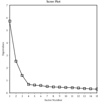
The 15 item parcels were subjected to an unrestricted maximum-likelihood factor analysis with oblique Promax rotation (k = 4). The Scree-plot suggested that three factors should be extracted (see Figure 1), which jointly explained 63.52% of the variance. Although the significant likelihood chi-square suggested that more factors might be extracted, c2(63) = 229,61, p < 0,001, inspection of the residual matrix showed only two residuals > 0,05 (see Table 6). The overall smallness of the residuals showed that the extraction of more factors was not warranted. Moreover, the extraction of only three factors was consistent with the theoretical measurement model that underlies the Locus of Control Inventory.
The Promax rotated factor pattern matrix is presented in Table 7. Inspection of this table shows that each factor was well defined: Factor 1 by item parcels A1 to A5, Factor 2 by item parcels I1 to I5, and Factor 3 by item parcels E1 to E5. The primary factor pattern coefficients ranged between 0,53 (I1 on Factor 2) and 0,82 (A2 on Factor 1). The highest secondary factor pattern coefficient of any parcel was 0.16 (A1 on Factor 2), suggesting that each parcel was a relatively pure indicator of its respective factor.
The correlations between the factors were as follows: Factor 1 (Autonomy) and Factor 2 (Internal Control), r= 0,64; Factor 1 (Autonomy) and Factor 3 (External Control), r= -0,38; and Factor 2 (Internal Control) and Factor 1 (External Control), r = -0,24.
Overall, the findings of the unrestricted factor analysis of the item parcels are consistent with the postulated structure of the Locus of Control Inventory and provide support for the construct validity of the three scales.
Figure 1. Scree plot of eigenvalues for the item parcel solution
Maximum-likelihood confirmatory factor analysis
The construct validity of the postulated factor structure of the Locus of Control Inventory was also examined with a maximum-likelihood confirmatory factor analysis. The first TABLE5
SKEWNESS AND KURTOSIS OF THE15 LOCUS OF CONTROL INVENTORY ITEM PARCELS
Parcel Skewness Kurtosis Parcel Skewness Kurtosis Parcel Skewness Kurtosis
E1 0,167 -0,444 I1 -0,294 0,048 A1 -0,374 -0,001
E2 0,114 -0,164 I2 -0,828 1,075 A2 -0,055 -0,078
E3 0,365 -0,095 I3 -0,550 0,334 A3 -0,236 -0,011
E4 0,090 -0,229 I4 -0,388 0,096 A4 -0,121 -0,048
E5 0,446 0,031 I5 -0,342 0,072 A5 -0,172 -0,220
Note. Mardia coefficient of multivariate kurtosis = 35,72; Normalised multivariate kurtosis = 32,242
TABLE6
STANDARDISED REESIDUAL MATRIX AFTER UNRESTRICTED MAXIMUM LIKELIHOOD EXTRACTION OF THREE FACTORS
E1 E2 E3 E4 E5 I1 I2 I3 I4 I5 A1 A2 A3 A4
E2 0,07
E3 -0,02 -0,04
E4 -0,01 0,04 -0,02
E5 -0,03 -0,04 0,07 -0,01
I1 0,00 -0,01 0,02 0,00 -0,01
I2 0,01 0,01 -0,03 0,01 0,01 -0,01
I3 0,01 0,00 0,01 -0,03 0,00 -0,02 0,00
I4 -0,01 0,00 0,02 0,00 -0,01 0,02 0,00 0,01
I5 -0,01 0,00 -0,01 0,02 0,01 0,01 0,01 0,01 -0,02
A1 -0,01 -0,01 0,01 0,00 0,00 -0,02 0,02 -0,02 0,00 0,00
A2 0,01 0,00 0,02 -0,02 -0,01 0,00 -0,01 0,03 0,00 -0,01 -0,01
A3 -0,02 -0,02 0,00 0,02 0,02 -0,01 -0,01 -0,01 0,00 0,01 0,01 0,00
A4 0,01 0,02 -0,02 0,02 -0,03 0,00 0,01 -0,02 0,00 0,00 -0,01 0,02 -0,01
A5 0,01 0,00 -0,01 -0,01 0,01 0,01 0,00 0,00 -0,01 0,00 0,01 0,00 0,00 -0,01
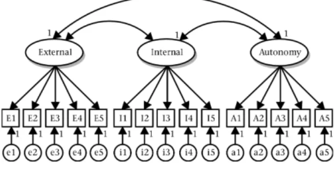
step in the confirmatory factor analysis was to specif y the measurement model (see Figure 2). This model, which was labelled Model 1, postulated that parcels E1 to E5 were indicators of an External Control factor, parcels I1 to I5 were indicators of an Internal Control factor, and parcels A1 to A5 were indicators of an Autonomy factor. Model 1 is consistent with the scoring key of the Locus of Control Inventory. In accordance with common factor theory, each parcel was also influenced by a unique factor that represented error variance and specific variance. The unique variances and the loadings of the factors on their respective indicators were freely estimated from the data. The loadings of a factor on the parcels that do not serve as indicator of that factor were constrained to zero (for instance the loading of Autonomy on parcel E1 was hypothesised to be equal to zero). The correlations between the factors were also freely estimated from the data. To statistically identif y the model, the variances of the factors and the regression weights of the parcels on the unique factors were fixed to unity. In the last place, the correlations between all unique factors were constrained to be equal to zero.
TABLE7
UNRESTRICTED PROMAX ROTATED FACTOR PATTERN MATRIX
(K= 4) OF ITEM PARCELS
Parcel Factor
1 2 3 h2
E1 -0,03 -0,07 0,67 0,49
E2 0,07 0,04 0,76 0,53
E3 0,06 -0,04 0,75 0,54
E4 -0,01 0,06 0,68 0,46
E5 -0,14 -0,02 0,66 0,53
I1 0,14 0,53 -0,04 0,41
I2 -0,14 0,81 -0,01 0,53
I3 -0,06 0,74 -0,10 0,53
I4 0,14 0,71 0,03 0,63
I5 0,07 0,71 0,10 0,54
A1 0,69 0,16 0,11 0,58
A2 0,82 -0,06 0,04 0,59
A3 0,76 0,02 0,04 0,53
A4 0,73 -0,09 -0,12 0,52
A5 0,75 0,06 -0,10 0,69
Note. Factor loadings > 0,15 are printed in bold face.
Figure 2: Confirmatory factor analysis model for the Locus of Control Inventory
The fit indices (see Appendix A for explanations of the fit indices) obtained in this study were as follows: c2 (87) = 628,51; Goodness of Fit Index (GFI) = 0,95; Adjusted Goodness of Fit Index (AGFI) = 0,93; Tucker-Lewis Index (TLI) = 0,94; Comparative Fit Index (CFI) = 0,95; Root Mean Square Error of Approximation (RMSEA) = 0,062 (,058 – 0,067); and Standardised Root Mean Squared Residual (SRMR) = 0,05. Although the hypothesis of an exact fit was rejected, the GFI, AGFI, TLI, CFI, RMSEA, and SRMR suggested satisfactory fit bet ween Model 1 and the data. The rejection of the hypothesis of exact fit was not unexpected, because with a sample size of 1662 the chi-square was rendered so powerful that even very small discrepancies would have led to a significant chi-square.
Inspection of the standardised residual matrix shows that, for the most part, the residuals were small (see Table 8). It does seem, however, that the External Control and Autonomy parcels share some variance that is not adequately modelled. The statistical fit of Model 1 could be improved by estimating the correlations bet ween the External Control and Autonomy unique variances. This was not done, however, because in the absence of theoretical justification for such correlations, they would have been difficult to explain.
The standardised estimated factor loadings of Model 1 are summarised in Table 9. Each of the factors had high and statistically significant loadings on their respective parcels, which shows that the parcels are good indicators of the constructs. The loadings ranged from 0,65 (I1 on the Internal Control factor) to 0,84 (A5 on the Autonomy factor). Note that these loadings, and therefore also the communalities, are higher than what would have obtained
TABLE8
STANDARDISED RESIDUAL MATRIX AFTER CONIRMATORY MAXIMUM LIKELIHOOD AXTRACTION OF THREE FACTORS
E1 E2 E3 E4 E5 I1 I2 I3 I4 I5 A1 A2 A3 A4
E2 0,07
E3 -0,03 -0,02
E4 -0,02 0,06 -0,01
E5 -0,04 -0,05 0,06 -0,02
I1 -0,08 0,00 -0,01 -0,01 -0,11
I2 -0,02 0,08 -0,01 0,06 -0,03 -0,02
I3 -0,08 0,01 -0,04 -0,03 -0,10 -0,02 0,03
I4 -0,06 0,08 0,04 0,05 -0,08 0,00 0,00 0,00
I5 0,00 0,12 0,06 0,12 0,00 0,00 0,03 0,01 -0,02
A1 0,02 0,14 0,12 0,10 -0,01 0,06 0,02 0,01 0,09 0,06
A2 0,00 0,10 0,08 0,02 -0,07 0,02 -0,10 -0,03 0,00 -0,03 -0,01
A3 -0,02 0,08 0,07 0,07 -0,04 0,03 -0,07 -0,03 0,03 0,01 0,02 0,01
A4 -0,08 0,01 -0,06 -0,02 -0,17 0,02 -0,09 -0,07 -0,02 -0,05 -0,02 0,04 0,00
A5 -0,07 0,03 -0,02 -0,03 -0,12 0,06 -0,05 -0,01 0,03 0,00 0,00 0,00 -0,01 0,00
if individual items served as the units of analysis. The correlations between the three factors were as follows: External Control and Internal Control, r = -0,27; External Control and Autonomy, r = -0,42; and Autonomy and Internal Control, r= 0,69.
TABLE9
STANDARDISED CONFIRMATORY FACTOR PATTERN MATRIX FOR THE15 PARCELS
Parcel External Internal Autonomy t-statistic
Control Control
E1 0,70 (0,02) 0,00 0,00 45,19*
E2 0,71 (0,02) 0,00 0,00 46,77*
E3 0,73 (0,02) 0,00 0,00 49,93*
E4 0,66 (0,02) 0,00 0,00 40,16*
E5 0,73 (0,02) 0,00 0,00 49,91*
I1 0,00 0,65 (0,02) 0,00 39,72*
I2 0,00 0,69 (0,02) 0,00 45,60*
I3 0,00 0,72 (0,01) 0,00 49,79*
I4 0,00 0,81 (0,01) 0,00 70,51*
I5 0,00 0,72 (0,02) 0,00 51,01*
A1 0,00 0,00 0,75 (0,01) 59,92*
A2 0,00 0,00 0,75 (0,01) 60,09*
A3 0,00 0,00 0,75 (0,01) 60,55*
A4 0,00 0,00 0,70 (0,01) 49,39*
A5 0,00 0,00 0,84 (0,01) 88,52*
Note. Standard errors of the factor pattern coefficients are given in parenthesis.
* p < 0,01
To provide a further basis for comparison, the confirmatory factor analysis was also conducted with the 77 items as the units of analysis (Model 2). Each item was assigned to a factor in accordance with the scoring key. Factor loadings and error variances were freely estimated, but the variances of the factors and the regression of the parcels on the unique factors were fixed to unity. The goodness of fit indices for Model 2 were as follows: c2(2846) = 12374,31; GFI = 0,80; AGFI = 0,79; TLI = 0,66; CFI = 0,67; RMSEA = 0,052 (0,052 – 0,053); and SRMR = 0,06. For all the indices, except the RMSEA and the SRMR, Model 2 (item model) fit the data substantially poorer than Model 1 (parcel model). To allow for quick comparison, the fit of the two models is summarised in Table 10.
TABLE10
COMPARISON OF FIT INDICES FOR ITEM VERSUS PARCEL BASED MEASUREMENT MODELS
Fit index Item model Parcel model
Chi square 12374,31 628,51
df 2846 87
Jöreskog and Sörbom GFI 0,80 0,95
Jöreskog and Sörbom AGFI 0,79 0,93
TLI 0,66 0,94
CFI 0,67 0,95
RMSEA 0,052 (0,052 – 0,053) 0,062 (0,058 – 0,067)
SRMS 0,06 0,05
Note. For the RMSEA 90% confidence intervals are given in parenthesis.
Overall, the confirmatory factor analysis of the item parcels revealed a good fit between the model and the data. The item parcels were shown to be strong indicators of their respective factors. The correlations between the factors were moderately
high to high. Note that Autonomy and Internal Control shared approximately 50% of their reliable variance, suggesting that they might be combined into a single factor. Inspection of the Modification Indices, however, showed that the fit of the model could not be improved by allowing the indicators of the two factors to have cross loadings or by allowing the unique factors of these indicators to be correlated. Moreover, a model where the correlation between the Autonomy and Internal Control factors was constrained to unity (Model 3), showed relatively poor fit: c2 (88) = 1170,46; GFI = 0,91; AGFI = 0,88; TLI = 0,88; CFI = 0,90; and RMSEA = 0,086 (,082 - 0,090). Because Model 3 was nested within Model 1, the difference in their respective chi-squares could be interpreted for significance. This difference was statistically significant, c2(1) = 542,13, suggesting that the original three-factor model (Model 1) fit the data significantly better than Model 3. These findings provide support for the construct validity of the three scales of the Locus of Control Inventory.
DISCUSSION
The purpose of this article was to examine problems encountered in the factor analysis of items and to demonstrate two methods that may be used to address these problems, namely item response theory models, and the factor analysis of item parcels rather than individual items. It was pointed out in the introduction that the problems might be attributed to the violation of some of the assumptions on which factor analysis is based. The first assumption is that the input data are continuous and measured on an interval level, but items provide ordinal data that typically contain only a limited number of ordered categories. Secondly, the distributions of items are often nonnormal, which violates the assumption of normality. Thirdly, the relations between items and the traits that underlie them are nonlinear, which violates the assumption of linear relations. Furthermore, in comparison to scales items are unreliable, which leads to low communalities, poor factor solutions, and correlated unique factors.
The factor analysis of items, the Rasch rating scale model, and the factoring of item parcels were applied to the items of the Locus of Control Inventory. This inventory consists of three scales, namely Autonomy, Internal Control and External Control. A central focus of this study was to examine the degree to which the different analytic methods support the construct validity of the three scales.
Unrestricted principal axis factor analysis of the Locus of Control Inventory items
On theoretical grounds one would expect three factors to explain the covariances of the 77 items of the Locus of Control Inventory. However, when subjected to a principal factor analysis the eigenvalues-greater-than-unity criterion suggested 19 factors. When the items of the three scales were analysed separately the eigenvalues-greater-than-unity criterion suggested five factors for the Autonomy scale, five factors for the Internal Control scale, and six factors for the External Control scale. On the basis of these results one might conclude that the scales are multidimensional rather than unidimensional and that their scoring keys may have to be revised to reflect this multidimensionality. However, it should be kept in mind that the observed multidimensional structure might be a methodological artefact. Nunnally and Bernstein (1994) warned in this regard:
Rasch rating scale analysis
The Rasch model represents a mathematical ideal for measurement, which requires that all the items should relate in a consistent way to the trait of interest. Only two factors influence an individual’s response to an item in the Rasch model: (a) the individual’s standing on the latent trait that the item measures, and (b) the difficulty or endorsability of the particular item. From this it follows that if the data fit the model, then the items constitute an essentially unidimensional scale.
The Rasch rating scale analysis of the Locus of Control Inventory items showed that with the exception of a small number of items, the fit between the data and the model was satisfactory for all three scales. Hence, it is concluded that each of the Autonomy, Internal Control and External Control scales measure an unidimensional trait and that the items in each scale function properly. These results are in contrast to that of the principal factor analysis of the same data, which suggested that the scales are multidimensional. A possible reason for the different results might be that the Rasch model was explicitly designed for the analysis of ordinal items and explicitly models non-linear relations between items and the latent trait that they measure, whereas factor analysis is more appropriate for the analysis of continuous, normally distributed data.
Some authors argue that it is not necessary to employ the Rasch or other item response theory models, because the person measures produced by these models correlate very strongly with ordinary summated total scores (Fan, 1998). One should note, however, that a very strong correlation is only observed if the data fit the Rasch model. Under these conditions the total score contains all the information necessary to estimate a person’s standing on the latent trait (Andrich, 1989). When the data do not fit the model, the total score is not a sufficient statistic for the estimation of a person’s standing on the latent trait and the correlation between total scores and the Rasch person measures will be lower. From this perspective the Rasch model provides justification for the calculation of total scores ifthe data fit the model. Rasch measures are to be preferred over total scores because total scores represent the ordinal-scale measurement, whereas Rasch measures are at an interval level. Furthermore, Rasch measures are independent of the particular sample of items, and as a consequence are not adversely affected by missing data. In the last place a Rasch analysis allows for the identification of individuals whose responses do not fit the model and for whom the total score might not be an adequate indicator of his or her standing on the latent trait.
Unrestricted factor analysis of the item parcels
The 77 items of the Locus of Control Inventory were reduced to 15 parcels through the random assignment of items within a particular scale to a parcel. Each parcel contained five or six items and each of the External Control, Internal Control, and Autonomy scales was represented by three parcels. Note that the parcelling was only performed after the Rasch analysis had supported the unidimensionality of the three scales. Hence, each parcel might be considered to be a mini-version of the full scale to which it belongs.
The unrestricted factor analysis of the 15 item parcels with Promax rotation provided strong support for the validity of a three-factor solution to the Locus of Control Inventory. These factors corresponded with the External Control, Internal Control, and Autonomy scales. The residual covariances of the parcels were very small indicating that no additional factors with substance could be extracted from them. These results are in contrast with those of the unrestricted principal axis factor analysis of the 77 items as described in the paragraphs above. The factor analysis of the parcels produced results that are in accordance with the theory that underlies the Locus of Control Inventory.
Confirmatory factor analysis of the item parcels
The effect of item parcelling in confirmatory factor analysis was investigated by comparing the results of an item-level confirmatory model with those of a parcel-level confirmatory model. In the
item-level model the 77 items served as indicators of the Internal Control, External Control, and Autonomy factors, and in the parcel-level model the 15 parcels served as the indicators of these three factors. A comparison of the two models showed that the parcel-level model fit the data much better than the item-level model. The fit of the parcel-level model was very good, indicating that the covariances of the parcels were adequately explained by the three postulated factors of the Locus of Control Inventory. In contrast, the results of the item-level analysis indicated poor fit.
The superior fit of the parcel-level model in the unrestricted and confirmatory factor analyses may be ascribed to the fact that parcels are more reliable, have more scale points, more closely approximate an interval-scale level, more closely approximate normality, and therefore more closely satisfy the assumptions of factor analysis than do individual items. In addition, parcels have proportionally smaller unique variances, which lessens the likelihood of correlations between unique factors.
One should consider the possibility that the parcelling procedure might have masked poorly fitting items and model mis-specification, but in this study the parcels were formed after the Rasch analysis had confirmed that a common thread runs through all the items in a particular scale. Hence, it appears safe to conclude that the random assignment of items to parcels was justified.
RECOMMENDATIONS
Taking into consideration the results of this study and the work of others, the following three-step strategy is recommended for the analysis of questionnaires or inventories with more than one scale (of which the Locus of Control Inventory is an example). This recommendation is based on the assumption that the scales were constructed on the basis of strong theory and that the researcher has a very clear idea of the constructs that each of the items serve to indicate.
As a first step, one should determine whether each of the scales measure a single dominant trait. A satisfactory fit between the data and the Rasch model, which was explicitly designed for the analysis of items, provides strong justification for the presence of such a dominant trait. The Rasch model may also be used to identify weak items that are in need of revision or items that should be eliminated from the scale.
As a second step, researchers may randomly assign the items within a scale to parcels. Note that the random assignment of items to parcels is only justified if the items within a scale measure a unidimensional or dominant trait. In the absence of unidimen-sionality it is not clear what parcels formed by random assignment represent and any further analysis of the parcels will be meaningless.
As a third step, the parcels may serve as the input variables for unrestricted or confirmatory factor analysis. If the results of the factor analysis correspond with the anticipated structure it provides support for the construct validity of the scales. In addition, the preceding analyses will have confirmed the quality of the items that comprise the scales. However, if the results do not correspond with the anticipated structure the construct validity of the scales should be questioned. It is possible that the original items do not serve as adequate indicators of the relevant constructs or it may be that the theory on which the scales are based may need to be revised.
REFERENCES
Andrich, D. (1978a). A rating scale formulation for ordered response categories. Psychometrika, 43, 561-573.
Andrich, D. (1989). Rasch models for measurement. Thousand Oaks, CA: Sage.
Bandalos, D.L. (2002). The effects of item parcelling on goodness-of-fit and parameter estimate bias in structural equation modelling. Structural Equation Modeling, 9, 78-102. Bernstein, I.H. & Teng, G. (1989). Factoring items and factoring scales are different: Spurious evidence for multidimensionality due to item categorization. Psychological Bulletin, 105, 467-477. Bond, T.G. & Fox, C.M. (2001). Applying the Rasch model: Fundamentals of measurement in the human sciences. Mahwah, NJ: Erlbaum.
Browne, M.W. & Cudeck, R. (1993). Alternative ways of assessing model fit. In K.A. Bollen & J.S. Long (Eds) Testing structural equation models(pp. 445-455). Newbury Park, CA: Sage. Byrne, B.M. (2001). Structural equation modeling with AMOS: Basic
concepts, applications and programming. Mahwah, NJ: Erlbaum. Cattell, R.B. & Burdsal, C.A. (1975). The radial parcel double
factor design: A solution to the item-versus-parcel controversy. Multivariate Behavioral Research, 10, 165-179. Comrey, A.L. (1970). The Comrey Personality Scales. San Diego,
CA: Edits.
Comrey, A.L. (1988). Factor analytic methods of scale development in personality and clinical psychology. Journal of Consulting and Clinical Psychology, 56, 754-761.
Embretson, S.E. & Reise, S.P. (2000). Item response theory for psychologists. Mahwah, NJ: Erlbaum.
Fan, X. (1998). Item response theory and classical test theory: An empirical comparison of their item/person statistics. Educational and Psychological Measurement, 58, 357-381. Finch, J.F. & West, S.G. (1997). The investigation of personality
structure: Statistical models. Journal of Research in Personality, 31, 439-485.
Fischer, G.H. (1995). Derivations of the Rasch model. In G.H. Fischer & I.W. Molenaar (Eds), Rasch models: Foundations, recent developments, and applications(pp. 15-38). New York: Springer-Verlag.
Floyd, F.J. & Widaman, K.F. (1995). Factor analysis in the development and refinement of clinical assessment instruments. Psychological Assessment, 7, 286-299.
Gorsuch, R.L. (1997). Exploratory factor analysis: Its role in item analysis. Journal of Personality Assessment, 68, 532-560. Hu, L. & Bentler, P.M. (1999). Cutoff criteria for fit indexes in
covariance structure analysis: Conventional criteria versus new alternatives. Structural Equation Modeling, 6, 1-55. Jöreskog, K.G. (1969). A general approach to confirmatory
maximum likelihood factor analysis. Psychometrika, 34, 183-202.
Jöreskog, K.G. & Sörbom, D. (1989). LISREL 7: A guide to the program and applications(2nded.). Chicago: SPSS Inc. Kishton, J.M. & Widaman, K.F. (1994). Unidimensional versus
domain representative parceling of questionnaire items. Educational and Psychological Measurement, 54, 757-765. Linacre, J.M. (2003). Winsteps. Chicago: MESA Press.
Linacre, J.M. & Wright. B.D. (1994). Reasonable mean square fit values. Rasch Measurement Transactions, 8(3), 370.
Little, T.D., Cunningham, W.A., Shahar, G. & Widaman, K.F. (2002). To parcel or not to parcel: Exploring the question, weighing the merits. Structural Equation Modeling, 9, 151-173. McDonald, R.P. (1999). Test theory. Mahwah, NJ: Erlbaum. Nunnally, J.C. & Bernstein, I.H. (1994). Psychometric theory. New
York: McGraw-Hill.
Rasch, G. (1960). Probalistic models for some intelligence and attainment tests. Copenhagen: Danmarks Paedagogiske Institut. Reise, S.P. (1999). Personality measurement issues viewed through the eyes of IRT. In S.E. Embretson & S.L. Hersberger (Eds), The new rules of measurement (pp. 219-242). Mahwah, NJ: Erlbaum. Schepers, J.M. (1992). Toetskonstruksie: Teorie en praktyk.
Johannesburg: RAU.
Schepers, J.M. (1995). Locus of Control Inventory. Johannesburg: RAU. Waller, N.G., Tellegen, A., McDonald, R.P. & Lykken, D. (1996).
Exploring non-linear models in personality assessment: Development and preliminary validation of a negative emotionality scale. Journal of Personality, 64, 545-576.
Wright, B.D. (1999). Fundamental measurement for psychology. In S.E. Embretson & S.L. Hershberger (Eds), The new rules of measurement: What every educator and psychologist should know (pp. 65-104). Mahwah, NJ: Erlbaum.
Wright, B.D. & Masters, G.N. (1982). Rating scale analysis: Rasch measurement. Chicago: MESA Press.
APPENDIX A
Goodness of fit of the confirmatory factor analysis models The fit between the hypothesised measurement model and the empirical data was evaluated by means of so-called goodness of fit indicators. The hypothesis of an exact fit was tested with the likelihood chi square, which states that the discrepancy between the observed covariances of the indicators (which may be items or parcels) and the covariances reconstructed on the basis of the model parameters are zero. Some authors argue that the exact fit test is too stringent, since it is unlikely that a hypothesised model will ever fit the data exactly (Browne & Cudeck, 1993; McDonald, 1999). Furthermore, with increasing sample size the chi-square test may become so powerful that even trivial differences between the two matrices may lead to the rejection of the hypothesised model (Byrne, 2001). This problem may be summarised as follows:
Such a hypothesis (of perfect fit) may be quite unrealistic in most empirical work with test data. If a sufficiently large sample were obtained this statistic would, no doubt, indicate that any such non-trivial hypothesis is statistically untenable. (Jöreskog, 1969, p. 200)
Several heuristic indicators of the “practical” fit between the model and the data have been devised. In this study the following indicators were used: Jöreskog and Sörbom’s Goodness of Fit Index (GFI) and Adjusted Goodness of Fit Index (AGFI), the Tucker-Lewis Indicator (TLI), the Comparitive Fit Index (CFI), the Root Mean Square Error of Approximation (RMSEA) and the Standardised Root Mean Squared Residual (SRMSR). The GFI and AGFI are measures of absolute fit between the model and the data. Loosely stated, the GFI reflects the proportion of variance accounted for by the proposed model and in this sense it is analogous to the R2of a multiple regression analysis. The AGFI is the GFI corrected for the complexity of the model, where models with less degrees of freedom are penalised. Generally, GFI and AGFI values greater than 0.90 are thought to indicate satisfactory fit.
The TLI and CFI compare the fit of the hypothesised model to that of a baseline model (which is usually an independance model where all variables are hypothesised to have zero covariances). The TLI and CFI generally range between zero and unity (the TLI can have values greater than unity in some cases) and a rule of thumb is that values of approximately 0.95 and higher indicate satisfactory fit (Hu & Bentler, 1999).
The RMSEA expresses the error of approximation per degree of freedom. Writing within the context of testing for exact fit versus testing for close fit (or practical fit), Browne and Cudeck (1993) summarised guidelines for interpreting the RMSEA as follows:
Practical experience has made us feel that a value of the RMSEA of about 0,5 or less would indicate a close fit of the model in relation to the degrees of freedom. This figure is based on subjective judgement. It cannot be regarded as infallible or correct, but is more reasonable than the requirement of exact fit with the RMSEA = 0,0. We are also of the opinion that a value of about 0.08 or less for the RMSEA would indicate a reasonable error of approximation and would not want to employ a model with a RMSEA greater than 0.1 (Browne and Cudeck, 1993).