Vol 60, No 4 (2017)

TECHNICAL UNIVERSITY OF CLUJ-NAPOCA

ACTA TECHNICA NAPOCENSIS

Series: Applied Mathematics, Mechanics, and Engineering Vol. 60, Issue IV, November, 2017

DYNAMICS CONTROL FUNCTIONS FOR A BALL SCREW

TRANSMISSION AXIS

Claudiu SCHONSTEIN, Iuliu NEGREAN

Abstract: In the paper, will be established the driving moment for a translational robot axis based on ball screw transmission. It is presented a detailed dynamic study of transmission gearing, and implicit a rigorous determination of the dynamic control functions, along the cinematic chain of the mechanical robotic system. The study is a fundamental aspect, with deep implications in optimal robot design in terms of sizing, power consumption and accuracy.

Key words: dynamics, ball screw, control, acceleration energy, polynomial interpolating functions. 1. INTRODUCTION

In achieving high performance of any mechanical structure, an important role is assigned to the transmission elements that make the connections between the mechanical system components. The mathematical modeling process is based on simplifying assumptions, in order to obtain workable and easy to use dynamic equations. One of the assumptions is the rigidity of the component elements of the structure, according to which the relative position and orientation of the components of each kinetic assembly does not change during the operation of the system. Another hypothesis is linked to negligible clearances, included in the precision of the mechanical ensemble.

The establishing of dynamic equations for a robotic system, mean to determine the motion equations for the constituting elements of the assembly, using fundamental notions in the advanced mechanics of the mechanical systems. A complete dynamic model includes the dynamic model of the robot's driving system and the dynamic model of the transmission chain.

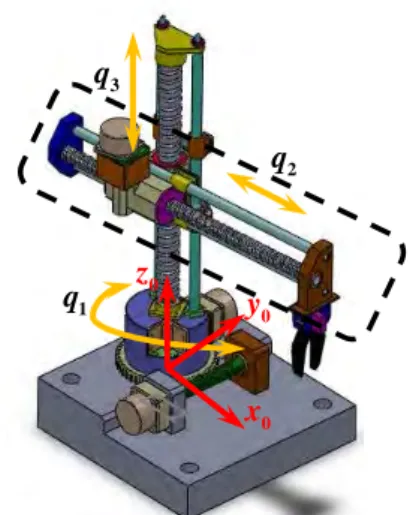
In the first part of the paper, based on the differential principles of advanced mechanics specific to mechanical olonomous systems, there is considered in Figure 1, a R2T serial robot structure.

Using advanced notions as the acceleration energy as presented in [1] and [2] there will be established analytically the generalized driving force for a horizontally axis. In the second part, there will be analyzed the transmission chain, whereas regardless of the type or complexity degree of the application where is implemented the robot structure, the performance accuracy imposed are increasingly larger. The third part is dedicated to graphically representation of the kinematical parameters and the driving moments for the considered axis, in the case of a working task performed by the robot.

Fig. 1 The R2T proposed serial structure

0 O 0 x

0 z

0 y

3 q

1 q

2

q

0

x

0

y

0

2. THE GENERALIZED DRIVING FORCE FOR A SERIAL ROBOT STRUCTURE

In order to determine the dynamics equations for the considered axis, according to [1]-[3], the moving differential equations for any mechanical system can be established by means of the differential principles considered as fundamental notions in the study of the dynamics of mechanical systems with links, on the basis of which is expressed the generalized driving force, as being:

i i i i

m i g SU

Q∗ Q Q Q

= F + + (1)

where, Qi_iF is the generalized inertia force, i SU Q is the generalized handling force, Qi_g and Qi_m∗ _are

generalized gravitational and generalized driving forces, which are characterizing every i 1= →3 driving joint of the proposed robot structure. In the study, there is used as fundamental notion of advanced mechanics the acceleration energy, which is integrated in the following expression of the generalized inertia force [1]:

n

i A i

i A

i 1

i i

E

Q E

q q =

∂ ∂  

= = _∑ _

∂_&& ∂_&&  

F ; (2) where,EiA =EiA

(

q ;q ;q ; j 1j & &&j j = →i

)

and

(

q ;q ;qj & &&j j

)

are generalized coordinates,

velocities and accelerations, for each joint of robot.

In the expression (1), the term Qi_iF is substituted by (2) based on acceleration energy,

(

)

i

A j j j

E q ;q ;q ; j 1& && = →i [1], [4] of each kinetic link belonging to mechanical structure, expressed as:

(

)

{

}

( )

i i T i

A j j j i C_i C_i

i T i * i i i * i

i i i i i i

i T i i * i

i i i i

T i T i i i T i i i

i i pi i i pi i i

1

E q ;q ;q M v v

2 1

I I

2 1

I 2

1

Tr I I

2

= ⋅ ⋅ ⋅ +

 

+ ⋅ ω ⋅ ⋅ ω + ω ×_ ⋅ ω_ +

 

+ ⋅ ω ⋅ ω ×_ ⋅ ω +_

 

+ ⋅ω ⋅ ω ⋅_ ⋅ ω − ω ⋅ ⋅ ω ⋅ ω_

& &

& &&

& &

&

(3)

In (3), M is the mass corresponding to each _i kinetic link of the robot, i *I_i represents the axial centrifugal inertia tensor and iI the inertia _pi

tensor planar centrifugal that characterizes the entire kinetic assembly

_{( )}

i , relative to the frame

_{{ }}

i , applied in the mass center of each linkC . In the same expression, _i iv_Ci and

i Ci

v& are the velocity and the acceleration of

mass center, iω_i and iω&_i are the angular velocity and acceleration of the kinetic link

_{( )}

i relative to the moving frame

_{{ }}

i attached to the robot. [2]

On the basis of expression (3), by particularization, the total acceleration energy for the considered R2T serial structure, is:

( ) ( ) ( )

{

}

3 _i

A A j j j

i 1

3 2

1 3 3 3 3

3 2

3 3 3 3

6 2 2

3 1

2 6 4

2 3

E t , t , t E q ,q ,q ; j 1 i

q 1,9722 10 q s(q ) q c(q )

5,2092 10 q c(q ) q s(q ) 760,4409 10 q 3,7317 q

1,8412 q 772,2409 10 q

= −

−

−

−

_{θ θ θ} ₌∑  _{= → ≡}

   

 

≡ ⋅ ⋅ ⋅_ ⋅ + ⋅ _+

 

+ ⋅ ⋅_ ⋅ − ⋅ _ +

+ ⋅ ⋅ + ⋅ +

+ ⋅ + ⋅ ⋅

& && _{& &&}

&& && &

&& &

&& &&

&& &

(4)

where sq_i =sin(q )_i and cq_i =cos(q )_i .

According to [4], there are determined for the second translational axis (see Figure1):

( )

( )

T

( )

2 0 0

2 2 _X2

C C A

2

2 2 2

Q J

E E E

d

3,6824 q

dt q q q

∗

θ = θ ⋅ θ =

∂  ∂ ∂

=   − = = ⋅

∂ ∂ ∂

 &  && &&

F F

(5)

( )

2 g

Q θ =0 (6)

( )

2 SU

Q θ =0 (7) the generalized inertia force (5), gravitational force (6), and the generalized handling force (7), for the kinematic axis belonging to the structure.

Substituting (5)-(7) in (1), the dynamic equation for the considered robot axis, is:

2

m 2

Q ∗ 3,6824 q

= ⋅&& (8)

and represents the the generalized driving force in analytical form on the output shafts of driving motor.

3 DRIVING MOMENTS FOR SECOND KINEMATIC AXIS OF R2T ROBOT

Further there is analyzed, the translation along x₂ axis of the R2T serial structure, presented in Figure1. In order to realize the translation, the transmission gearing consisting in a worm gear which meshes with a toothed wheel, fixed jointly with the ball screw`s nut.

The analysis of the motor torque required to move the second coupling is expressed as the driving moment of the nut generated by the axial force of the contact between the worm and the worm gear. There is considered the first subassembly consisting of the screw that performs a rotation motion, and the nut that performs the translation, as in Figure 2.

According to [5], in ball screw transmission the stress is manifested by an axial force transmitted through balls, considered uniformly spread over the number of balls n_b of the working area, along the n_i axis (line joining the points of contact between the ball – nut, respectively ball – screw)

3.1 Establishing of screw`s driving moment The driving moment necessary to translation motion is due to the torque of the screw, which is generated by the axial force of the contact between the worm and the worm wheel. First, is determined the driving moment of the nu, then is established the axial force at the contact between worm and the worm wheel.

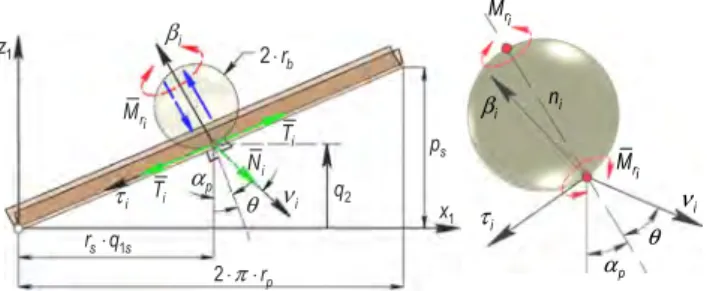
In concordance with Figure 3 depending on the helix of the nut’s threadα_p, there is written:

p ₂

p

p p 2p

p _q

tg

2 r r q

α = =

⋅ π ⋅ ⋅ (9)

where r_pis the radius of the nut, p_p thread pitch of the nut, and q₂ the generalized coordinate.

In keeping with the previous expression, the rotation angle of the screw is determined as:

2p 2

p

2

q q

p ⋅ π

= ⋅ (10) where q₂ =q₂

_{( )}

τ is a polynomial function of

the robot coordinates from the driving joint [2] hence, the angular velocity and acceleration of the screw are expressed:

( )

( )

( )

( )

2p 2 2p 2

p p

2 2

q q ; q q

p p

⋅ π ⋅π

τ = ⋅ τ τ = ⋅ τ

& & && && (11)

According to Figure 2, and knowing the number of the balls contained by the ball screw assembly n , as well as the rolling friction _b coefficient µ_sbp between the screw-balls,

respectively balls-nut, is determined the generalized driving force of the ball screw as:

2 nb

₍

₎

m i p sbp p

i 1

Q N c s

=

=∑ ⋅ α − µ ⋅ α (12) where θ represents the contact angle, having a direct influence on this type of transmission.

According to [6], the optimal value of the contact angle is θ =0, but considering that it is very difficult from technological point of view the achievement of this value, the producing companies are realizing these transmissions with a value of θ = π 4. Knowing the fact that between balls and screw/nut is appearing a rolling friction, the resistant moment in the screw-nut assembly, is:

n_b n_b

2

mfp i p p sbp i p p

i 1 i 1

nb

r_i p

i 1

Q N r s N r c

M s c 0

= =

=

+∑ ⋅ ⋅ α − µ∑ ⋅ ⋅ ⋅ α −

−∑ ⋅ θ⋅ α =

(13)

In the previous relation, the rolling friction moment is expressed as following:

i

n

p

α

ri

M

θ

i

ν

i

τ

i

β

ri

M

i

β

i T 1

z

p

α

2 q

1 x i

T ri M

2⋅ ⋅π rp

θ νi

2⋅r_b

1 s s r q⋅

s p i

N

i

τ

Fig.3 The ball-screw evolvent

2

q&

1p

q&

2

q

2

q

&&

1p

q

&&

2

x

2

y

2

m

Q

2

mp

Q

2

O

2

z

2

mfp

Q

r_i i b sbp

M =N r⋅ ⋅ µ (14) where, r_b is the radius of a ball.

Substituting the expression of the rolling friction moment in (13), the resistant moment in the screw-nut assembly is rewritten in final form as:

p sbp p

2 2

mfp m p

p sbp p

p b

sbp

p p sbp p

c s c

Q Q r

c c s

c r

s

r c c s

θ ⋅ α − µ ⋅ α



= − ⋅ ⋅ −

θ⋅ α + µ ⋅ α



α 

− ⋅µ ⋅ θ⋅ 

θ⋅ α + µ ⋅ α _

(15)

Knowing the radius of the worm wheel r_2m (fixed with the nut), and r_p the radius of the nut, there can be approximated the mechanical axial inertia moment of the assembly screw-worm wheel, equivalent with:

2 ₂

p p

2 2m 2m

2p

M r _{M r}

I

2 2

∗ ₌ ⋅ ₊ ⋅ _{, (16)}

where M and _p M_2m are the mass of the nut, respectively of the worm wheel.

According to the same Figure 2, in keeping with angular momentum theorem, there is written the identity:

( )

( )

( )

2 2 2

2p 2p mp mfp

I∗ q Q Q

⋅&& τ = τ + τ (17)

Considering the mechanical axial inertia moment of the assembly nut-worm wheel 2I2p∗ , defined with (16), as well as the angular acceleration of the ball screw (11), the driving moment of the ball screw is:

( )

( )

( )

( )

( )

2 2 2 2

mp 2p 2p mfp 2p 2

p

p sbp p

2

m p

p sbp p

p b

sbp

p p sbp p

2

Q I q Q I q

p

c s c

Q r

c c s

c r

s

r c c s

∗ ∗ ⋅π

τ = ⋅ τ − τ = ⋅ ⋅ τ +

θ⋅ α −µ ⋅ α



+ τ ⋅ ⋅ − θ⋅ α +µ ⋅ α



α 

− ⋅µ ⋅ θ⋅ 

θ⋅ α +µ ⋅ α _ && &&

(18)

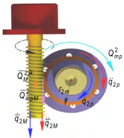
3.2 Establishing the axial force at the contact between the worm and the worm wheel To determine the axial force at the contact between the worm and the worm wheel, there is considered the second assemble presented in Figure 4.

Further is determined the angular velocity and acceleration of the worm, and implicitly of the shaft of the driving motor, as:

( )

( )

( )

( )

( )

2

2M 2m 2 2m 2

2M 2M p

2

2M 2m 2

2M p

2 4

q r q r q ;

p p p

4

q r q

p p

⋅π ⋅π

τ = ⋅ ⋅ τ = ⋅ ⋅ τ

⋅

⋅π

τ = ⋅ ⋅ τ

⋅

& & &

&& &&

(19)

where p_2Mis the worm`s step.

The axial force at the contact between the worm and worm wheel is:

( )

( )

2 2

mpM mp

2m 1

Q Q

r

τ = ⋅ τ (20)

In keeping with the fact that are known the values of the helix of the worm α_2M, as well as the sliding friction coefficient µ_2M between the worm and worm wheel, there can be written:

( )

{

( )

p sbp p

2 2

mfpM m p

p sbp p

p b

sbp

p p sbp p

2 2M 2M 2M 2M

2p 2

p 2m 2M 2M 2M

c s c

Q Q r

c c s

c r

s

r c c s

r s c

2

I q

p r c s

∗

θ⋅ α −µ ⋅ α



= − τ ⋅ ⋅ −

θ⋅ α +µ ⋅ α



α 

− ⋅µ ⋅ θ⋅ −

θ⋅ α +µ ⋅ α _

α −µ ⋅ α

⋅π 

− ⋅ ⋅ τ ⋅_ ⋅

α +µ ⋅ α

 &&

(21)

is the resistant moment of the worm wheel.

3.3 Determining the driving force that moves the nut

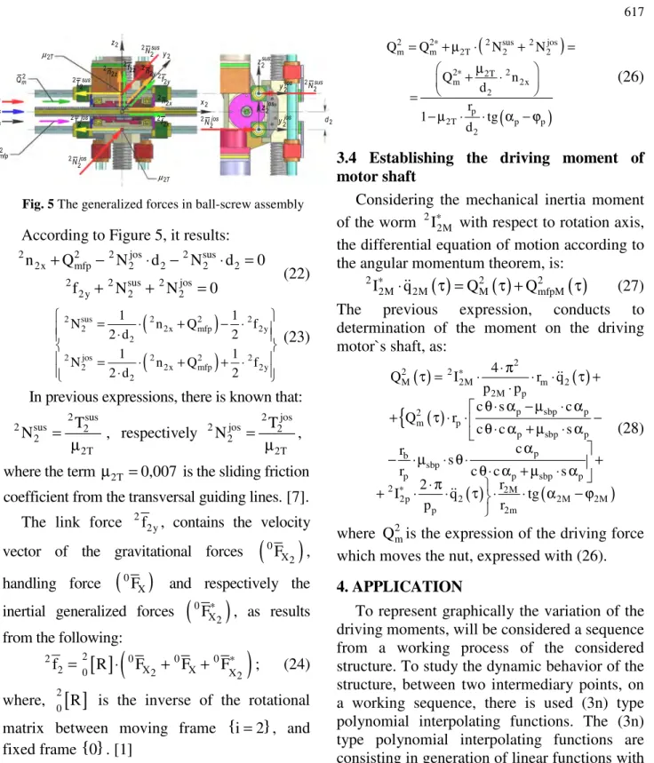
The resistant moment from ball screw assembly becomes driving moment for the screw, as shown in Figure 5. In order to establish the driving force that moves the nut, further there will be written the dynamic equilibrium equations for the nut.

&_2M

q

2p

q&

&&_2M

q

2p

q&&

2

m pM

Q

2

m p

Q

2jk M

Q

2m

r

Fig. 4 The gearing wheel –worm

According to Figure 5, it results:

2 2 2 jos 2 sus

2x mfp 2 2 2 2

2 2 sus 2 jos

2y 2 2

n Q N d N d 0

f N N 0

+ − ⋅ − ⋅ =

+ + = (22)

(

)

(

)

2 sus 2 2 2

2 2x mfp 2y

2

2 jos 2 2 2

2 2x mfp 2y

2

1 1

N n Q f

2 d 2

1 1

N n Q f

2 d 2

  = ⋅ + − ⋅  _⋅       _{= ⋅ + + ⋅}   ⋅    (23)

In previous expressions, there is known that:

2 sus 2 jos

2 sus 2 2 jos 2

2 2

2T 2T

T T

N = , respectively N =

µ µ ,

where the term µ_2T =0,007 is the sliding friction coefficient from the transversal guiding lines. [7].

The link force 2 2y

f , contains the velocity vector of the gravitational forces

(

0

)

X2 F ,

handling force

(

0

)

X

F and respectively the inertial generalized forces

(

0F_X2∗

)

_{, as results}

from the following:

[ ]

(

)

2

2 0 0 0

2 0 X2 X _X2

f R F F F∗

= ⋅ + + ; (24)

where, 2₀

_{[ ]}

R is the inverse of the rotational matrix between moving frame {_{i 2=} }_{, and}

fixed frame { }0 . [1]

The moment of linkage forces between the elements (_{i 1−} ) _and ( )_{i , applied to the origin}

of the frame { }_{i is:}

[ ]

(

)

2

2 0 0 0

2x ₀ X₂ X _X2

n ₌ R _⋅ N ₊ N ₊ N∗ ₍₂₅₎

and contains the resultant moments of the gravitational, handling and inertia system of forces.

The driving force necessary to generate the translation motion along x axis of the nut is: ₂

(

)

(

)

2 2 2 sus 2 jos

m m 2T 2 2

2 2T 2

m 2x

2

p

2T p p

2

Q Q N N

Q n d r 1 tg d ∗ ∗

= + µ ⋅ + =

µ   + ⋅     =

− µ ⋅ ⋅ α − ϕ

(26)

3.4 Establishing the driving moment of motor shaft

Considering the mechanical inertia moment of the worm 2I_2M∗ _{with respect to rotation axis,}

the differential equation of motion according to the angular momentum theorem, is:

( )

( )

( )

2 2 2

2M 2M M mfpM

I∗ q Q Q

⋅&& τ = τ + τ (27)

The previous expression, conducts to determination of the moment on the driving motor`s shaft, as:

( )

( )

( )

{

( )

(

)

2 2 2

M 2M m 2

2M p

p sbp p

2

m p

p sbp p

p b

sbp

p p sbp p

2 2M

2p 2 2M 2M

p 2m

4

Q I r q

p p

c s c

Q r

c c s

c r

s

r c c s

r 2

I q tg

p r

∗

∗

⋅ π

τ = ⋅ ⋅ ⋅ τ +

⋅

θ⋅ α − µ ⋅ α



+ τ ⋅ ⋅ −

θ ⋅ α + µ ⋅ α



α 

− ⋅µ ⋅ θ ⋅ _+

θ⋅ α + µ ⋅ α _

⋅ π 

+ ⋅ ⋅ τ _⋅ ⋅ α − ϕ



&&

&&

(28)

where Q2_mis the expression of the driving force which moves the nut, expressed with (26).

4. APPLICATION

To represent graphically the variation of the driving moments, will be considered a sequence from a working process of the considered structure. To study the dynamic behavior of the structure, between two intermediary points, on a working sequence, there is used (3n) type polynomial interpolating functions. The (3n) type polynomial interpolating functions are consisting in generation of linear functions with respect to time for generalized accelerations in the considered axis of the robot.

According to [8], [9], [4] is generated a linear function with respect to time as:

( )

m

(

)

m 1

( )

2m 2m m 1 2m m

m m

q q q

t t

− −

τ −τ τ−τ

τ = ⋅ τ + ⋅ τ

&& && && (29)

where t_m = τ − τ_{m m 1−} represents the duration

of each

(

m 1= →3

)

segment of the trajectory. Fig. 5 The generalized forces in ball-screw assembly

2 d 2 z 2 jos y 2 y 2s q 2s q& 2s q&& 2 2 jos T 2 2 sus N 2 2 sus T 2 2 jos N 2T µ 2T µ 2 2x n 2 2z

The unknowns are the generalized accelerations atτ_{m 1−} and τ_m, defined as:

(

)

( )

2m m 1 2m 1 2m m 2m

q τ ₋ = q ₋ ; q τ = q

&& && && && . (30)

After a few transformations, are obtained the functions for generalized velocities and coordination as shown:

( )

(

)

(

)

2 2

m m 1

2m 2m 1 2m

m i

2m m 2m 1 m

2m 2m 1

m m

q q q

2 t 2 t

q t q t

q q

t 6 t 6

− −

−

−

τ −τ τ−τ

τ = − ⋅ + ⋅ +

⋅ ⋅

   

+ − ⋅ − − ⋅ 

   

& && &&

&& &&

(31)

( )

(

)

(

)

(

)

(

)

3 3

m m 1

2m 2m 1 2m

l i

2m m 2m 1 m

2m m 1 2m 1 m

m m

q q q

6 t 6 t

q t _q q t _q

t 6 t 6

− −

−

− −

τ −τ τ−τ

τ = ⋅ + ⋅ +

⋅ ⋅

   

+ − ⋅ ⋅ τ−τ + − ⋅ ⋅ τ −τ

   

&& &&

&& &&

(32)

In order to express the driving moments of the mobile structure, the input parameters for study are presented as follows in the Table 1, where is considered that the first sequence is a translation along +Ox, and the second sequence is a translation along -Ox.

Table 1 Seq. Time

m s

τ

Duration m t s

Coordinates values

2m

q m

Translation along +Ox

9 0 0,125

10 1 11 1

12 1 0,25

Translation along -Ox

35,5 0 0,25

36,5 1 37,5 1

38,5 1 0,125

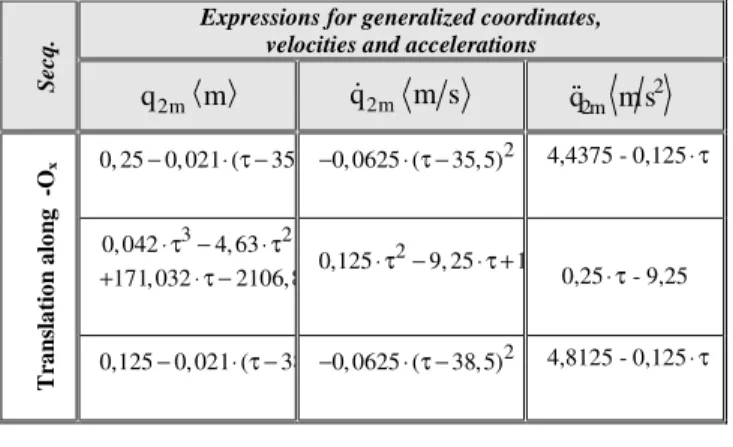
On the basis of the parameters presented in Table 1 in keeping with (30)-(32), are determined the expressions for coordinates, velocities and accelerations as seen in Table 2.

Table 2

S

ec

q

. Expressions for generalized coordinates, _{velocities and accelerations}

2m

q m q&2m m s &&q2m ms2

T

ra

n

sl

a

ti

o

n

a

lo

n

g

+

Ox

3 0, 21 ( 9)

0,125

⋅ τ − +

+ ₂

0,063 (⋅ τ −9) 0,125 - 1,125⋅ τ

3 2

0,042 1,312 13,69 47, 44

− ⋅ τ + ⋅ τ − ⋅ τ +

2 0,125 2,63 13,69

− ⋅ τ + ⋅ τ −

+ _{2,625 - 0,25⋅ τ}

3

0,021 (⋅ τ −12) +0, 25 ₂

0,0625 (⋅ τ −12) 0,125 - 1,5⋅ τ

S

ec

q

. Expressions for generalized coordinates, _{velocities and accelerations}

2m

q m q&2m m s q&&2m ms2

T

ra

n

sl

a

ti

o

n

a

lo

n

g

-O

x 0, 25 0,021 (− ⋅ τ −35,5)−0,0625 (⋅ τ −35,5)2 4,4375 - 0,125⋅ τ

3 2

0,042 4,63 171,032 2106,89

⋅ τ − ⋅ τ + ⋅ τ −

2

0,125⋅ τ −9, 25⋅ τ +171,0313_{0,25 - 9,25}

⋅ τ

0,125 0,021 (− ⋅ τ −38,5)−0,0625 (⋅ τ −38,5)2 4,8125 - 0,125⋅ τ

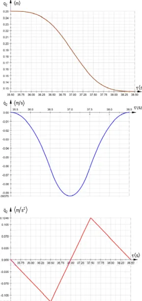
On the basis of Table 2, there are represented graphically, the generalized coordinates, velocities and accelerations, as in Figure 6 and Figure7.

2

q m

s

τ

s

τ

2

q m s

&

2 2

q m s

&&

s

τ

Fig. 6 The variation of kinematical parameters in

Taking into account the expression (28), where are known all the constructive and dynamic parameters of the component parts of the transmission gearing [4], and the input data contained in Table 1 and Table 2, there are determined the numerical value for the driving moments on the motor shaft, necessary to move the axis:

( )

x/ x

M 2

Q 0,04719029335 q -0,0000004469021

+ −

τ = ⋅&& ₍₃₃₎

As it can be seen from previous expression, (33) the total driving moment, has a dynamic respectively a static component.

On the basis of the same expression (33) are represented graphically the variation for the

driving moments, as results from Figure 8 and Figure 9.

4. CONCLUSION

The paper presents a detailed study concerning the dynamic behavior of a translational robot axis based on ball screw transmission. Using the acceleration energy as fundamental notion and the algorithm of generalized forces, in the first part of the paper it was analytically established the generalized driving moment for a horizontally axis belonging to a serial robot, without taking into account the transmission system of the structure from the driving motor to the kinematic chain. This generalized driving moment, had been included in the expression of the driving

2

q m

s

τ

s

τ

2

q& m s

2 2

q m s

&&

s

τ

Fig. 7 The variation of kinematical parameters in

translation along -Ox

Fig. 8 The variation of driving moment in

translation along +Ox

Qm N m⋅

τs

Total value of driving moment Dynamic value of driving moment Static value of driving moment

Qm N m⋅

τs

Fig. 9 The variation of driving moment in

moment of the motor shaft, established in the second part of the paper.

In the second part, was analyzed the transmission gearing, in keeping with the motion transmission chain. Hence, it has been presented the transmission gearing consisting in a worm gear which meshes with a toothed wheel, fixed with a ball screw, which interacts with a nut. For each subassembly, there have been established the analytical form of the moments, in keeping with the parameters of the considered kinematic axis, with the observation that in determining of the moments it were considered the specific existing frictions in mechanical transmission system.

In the last part of the paper, the analytical form of the driving moment motor it has been represented graphically. For this, it was considered two sequences of working task for the robot. The trajectory on considered sequences was divided into three segments, for each sequence, having as input data the displacement of the kinetic link and the correspondent time. Using the

( )

3n type polynomial interpolating functions there have been established the variation laws for accelerations, component of the driving moment on the motor shaft.

An important remark is that generally through an accurate and real determination of the driving moment the motors necessary for the operation of the kinematic axis, or the braking systems related can be sized rigorously, thus enabling to avoid critical situations, which can lead to damage of mechanical structure.

5. REFERENCES

[1] I., Negrean, Mecanică Avansată în Robotică, Editura UT PRESS, Cluj-Napoca, 2008, ISBN 978-973-662-420-9.

[2] Negrean, I., Schonstein, C., Kacso, K., Duca, A., Formulations in Advanced Dynamics of Mechanical Systems, The 11 th IFTOMM International Symposium on Science of Mechanisms and Machines, Mechanisms and Machine Science 18, DOI:10.1007/978-3-319-01845-4-19 Springer International Publishing Switzerland, pp. 185-195.

[3] D. Ardema, ”Analytical Dynamics Theory and Applications”, Springer US, ISBN 978-0-306-48681-4, pp. 225-243, 245-259, 2006. [4] Schonstein, C., Contribuții în dezvoltarea unei

structuri robotizate hibride, PhD Thesis, Cluj-Napoca, 2011.

[5] Pelecudi, Ch., Precizia mecanismelor, Editura Academiei Romane, Bucureşti, 1975.

[6] Gafiteanu, M., s.a., Organe de masini, vol 1, Editura Tehnică, Bucuresti, 1981.

[7]http://www.roymech.co.uk/Useful_Tables/Tribol ogy/co_of_frict.htm

[8] Negrean, I, Vuşcan, I, Haiduc, N, Robotică. Modelarea cinematică şi dinamică, Editura Didactică şi Pedagogică, R.A., Bucureşi, 1997.

[9] Fu, K., Gonzales, R. and Lee, C., Robotics: Control, Sensing, Vision and Intelligence, McGraw-Hill Book Co., International Edition, 1987.

Funcţii de control dinamic pentru o axă de transmisie cu şurub cu bile

În lucrare, se vor stabili momentele motoare pentru o axă de translaţie orizontală cu șurub cu bile a unui robot. Se

prezintă un studiu dinamic detaliat al mecanismului de transmisie și implicit o determinare riguroasă a funcțiilor de

control dinamic, de-a lungul lanțului cinematic al sistemului mecanic robotizat. Studiul are un aspect fundamental, cu implicații profunde în designul optim al unui robot în ceea ce privește dimensionarea, consumul de energie și precizia. Claudiu SCHONSTEIN, Lecturer, Ph.D, Eng, Technical University of Cluj-Napoca, Department of

Mechanical Systems Engineering, E-mail: [email protected], No.103-105, Muncii Blvd., Office C103A, 400641, Cluj-Napoca.

Iuliu NEGREAN Professor Ph.D., Member of the Academy of Technical Sciences of Romania,

Director of Department of Mechanical Systems Engineering, Technical University of Cluj-Napoca,