Econ Journal Watch
Scholarly Comments on Academic Economics
Volume 5, Issue 2, May 2008Comments
The Soviet Economic Decline Revisited,
Brendan K. Beare 135-144
Reply to Beare,
William Easterly and Stanley Fischer 145-147
The Diluted Economics of Casinos and Crime: A Rejoinder to Grinols and Mustard’s Reply,
Douglas M. Walker 148-155
Connecting Casinos and Crime: More Corrections of Walker
Earl L. Grinols and David B. Mustard 156-162
Smoking in Restaurants: Rejoinder to Alamar and Glantz
David R. Henderson 163-168
Externalities in the Workplace: A Response to a Rejoinder to Response to a Response to a Paper,
Benjamin C. Alamar and Stanton A. Glantz 169-173
InvestIgatIngthe apparatus
symposIum: genderand eConomICs Reaching the Top?
On Gender Balance in the Economics Profession,
On Gender Balance in the Economics Profession,
Ann Mari May 193-198
Mr. Max and the Substantial Errors of Manly Economics,
Deirdre N. McCloskey 199-203
Diversity in Tastes, Values, and Preferences: Comment on Jonung and Ståhlberg,
Catherine Hakim 204-218
Preferences Underlying Women’s Choices in Academic Economics,
John A. Johnson 219-226
What is the Right Number of Women?
Hints and Puzzles from Cognitive Ability Research,
Garett Jones 227-239
Christina Jonung and Ann-Charlotte Ståhlberg will reply in the September 2008 issue.
CharaCter Issues
Honestly, Who Else Would Fund Such Research? Reflections of a Non-Smoking Scholar,
Michael L. Marlow 240-268
B
rendanK. B
eare1a commenton: Wiliam eaSterly anD Stanley FiScher, “the Soviet economic Decline,” World Bank Economic rEviEW 9(3), September 1995: 341-371.
abStract
IntheIrpaper “the SovIet economIc declIne”, puBlIShedInthe World Bank Economic Review in 1995, William Easterly and Stanley Fischer study the decline of the Soviet economy during the period 1950-1987. The authors begin by showing that, conditional on standard growth determinants such as national investment and human capital accumulation, Soviet per capita economic growth was the worst in the world, and worsening, 1960-1987. This is despite the fact that during the 1950s Soviet growth per capita was significantly above the world average. The purpose of Easterly and Fischer’s study is to explain this poor economic performance. Two candidate explanations—that the Soviet economy was overly burdened by excessive military spending, and that central planning stymied the effectiveness of spending on research and development—are briefly considered, but Easterly and Fischer find that neither provides a plausible explanation for the extreme nature of the Soviet experience.
Instead, Easterly and Fischer focus on an explanation for the Soviet growth slowdown known as the extensive growth hypothesis, or low elasticity of substitution hypothesis. Extensive growth refers to growth that is driven primarily by input accu-mulation rather than productivity growth. As discussed by Easterly and Fischer, the decline in Soviet economic growth after the 1950s was accompanied by a substantial increase in the national investment rate, which more than doubled between 1950 and
1 Postdoctoral Prize Research Fellow, Nuffield College, University of Oxford. Oxford, UK OX1 1NF. The first version of this comment was written while the author was a graduate student in the Depart-ment of Economics at Yale University. I thank Timothy Guinnane, Valery Lazarev, Peter Phillips, an EJW reader, and an anonymous referee for their comments, and Yale University and the Cowles Foundation for financial support. The opinions expressed here are my own.
The Soviet Economic Decline Revisited
brenDan K. beare
1987. Similar increases in the investment rate were experienced in a number of newly industrializing East Asian economies, including Japan and Korea. Whereas extensive growth via capital accumulation led to rapid economic growth in much of East Asia, the rising investment rate in the Soviet economy was accompanied by a declining rate of growth. The extensive growth hypothesis, proposed earlier by Weitzman (1970), posits that this decline was due to sharply diminishing returns to capital brought about by a low elasticity of substitution between capital and labor. Easterly and Fischer argue that the elasticity of substitution was indeed much lower in the Soviet economy than in the newly industrializing East Asian economies, and suggest that the difference may be fundamentally related to the contrasting nature of planned and market economies.
The model of the Soviet economy used by Easterly and Fischer is a constant elasticity of substitution (CES) growth equation:
€
lnYt= d0+ d1t50−59+ d2t60−69+ d3t70−79+ d4t80−87+ g
g −1lnaKt g −1
( )/g+
(
1− a)
L tg −1( )/g
[
]
(1)
This is labeled as equation 6 in Easterly and Fischer’s paper (with ln Lt subtracted from both sides of the equation). In each period t, Yt denotes output, Kt denotes capi-tal, and Lt denotes labor. t50-59is equal to the product of t and a dummy variable that is equal to one in periods corresponding to the years 1950 to 1959, and equal to zero in other periods. The other trend variables are defined similarly. The parameters a, g ∈ (0,1) correspond to the share of capital in production and the elasticity of substitution between capital and labor. The log of technology, assumed by Easterly and Fischer to be Hicks-neutral, is equal to the sum of the first five terms on the right hand side of (1). Thus, d1 through d4 represent decade-specific rates of technical change. The pur-pose of the decade-specific trend functions is to allow for a modicum of flexibility in the evolution of technological progress over the sample period.
Easterly and Fischer seek to appraise the extensive growth hypothesis by empirically estimating (1) using nonlinear least squares. In a CES model of eco-nomic growth, an elasticity of substitution below one implies decreasing returns to capital accumulation. Thus, an estimate of g significantly (in both the statisti-cal and the economic sense) below one would provide support for the extensive growth hypothesis. Relatively constant estimates of d1 through d4 would provide further support for the extensive growth hypothesis, by showing that the bulk of the decline in Soviet growth can be explained by decreasing returns to capital ac-cumulation. An estimate of g close to one, and declining estimates of d1 through d4, would provide evidence against the extensive growth hypothesis.
from various sources.2 Three main sources are involved: a dataset constructed by
the U.S. Central Intelligence Agency (CIA), a dataset constructed by the Russian economist Khanin, and the official Soviet statistics.3 Easterly and Fischer report
estimates of (1) using the CIA data at the total economy and industrial sector lev-els. They also discuss briefly the results obtained using the other datasets.
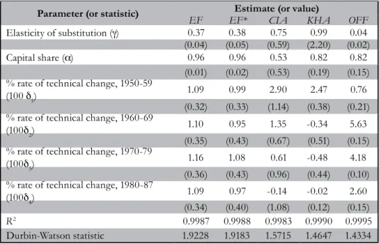
The results of Easterly and Fischer’s analysis using the CIA total econo-my data are displayed in the column labeled EF in Table 1. These estimates are taken from Table 6 in their paper. Using the original data and the equation they specified,4 I attempted to derive the same estimates. My own estimates are
dis-played in the column labeled EF* in Table 1. The figures in columns EF and EF* are similar, but not identical. Without the precise details of the numerical optimi-zation routine used by Easterly and Fischer, or access to the code used to generate their results, it is difficult to know exactly why the figures differ. Note that the R-squared values in columns EF and EF* are extremely close to one another. See McCullough and Vinod (2003) for a discussion of numerical discrepancies aris-ing from differences between econometric software packages and optimization settings. The figures in column EF* were obtained by performing a grid search over the nonlinear parameters g and a, running from 0.01 to 0.99 in increments of 0.01, and estimating the other parameters by linear regression conditional on g and a at each point in the grid. This approach was used to avoid the sensitivity of results to the choice of starting values in more sophisticated optimization rou-tines, a problem which appears to be substantial in this instance.
The estimates in column EF appear to provide striking support for the extensive growth hypothesis. The estimated elasticity of substitution is 0.37; well below one. Moreover, the estimated standard error for this parameter is only 0.04. The capital share parameter is estimated at 0.96, with a standard error of only 0.01. This estimate seems extremely high, even in view of the intensive capital accu-mulation in the Soviet economy during the sample period. The rates of technical change are less precisely estimated than the other parameters, but it is notable that they do not appear to decline over the sample period. The same qualitative state-ments hold true for our own estimates reported in column EF*.
2 The data are downloadable from the World Bank website: www.worldbank.org.
brenDan K. beare
Table 1: Parameter Estimates for the Soviet Production Function, 1950-1987
Parameter (or statistic) Estimate (or value)
EF EF* CIA KHA OFF
Elasticity of substitution (g) 0.37 0.38 0.75 0.99 0.04 (0.04) (0.05) (0.59) (2.20) (0.02)
Capital share (a) 0.96 0.96 0.53 0.82 0.82
(0.01) (0.02) (0.53) (0.19) (0.15) % rate of technical change, 1950-59
(100 d1)
1.09 0.99 2.90 2.47 0.76
(0.32) (0.33) (1.14) (0.38) (0.21) % rate of technical change, 1960-69
(100d2) 1.10 0.95 1.35 -0.34 5.63
(0.35) (0.43) (0.67) (0.51) (0.15) % rate of technical change, 1970-79
(100d3) 1.16 1.08 0.61 -0.48 4.18
(0.36) (0.43) (0.96) (0.44) (0.10) % rate of technical change, 1980-87
(100d4) 1.09 0.97 -0.14 -0.02 2.60
(0.34) (0.40) (1.08) (0.12) (0.15)
R2 0.9987 0.9988 0.9983 0.9990 0.9995
Durbin-Watson statistic 1.9228 1.9183 1.5715 1.4647 1.4334 Note: Estimated standard errors in parentheses. EF: Easterly-Fischer estimates based on CIA total economy data, equation (1); EF*: Author’s estimates based on CIA total economy data, equation (1); CIA: Author’s estimates based on CIA total economy data, equation (2); KHA: Author’s estimates
based on Khanin material sector data, equation (2); OFF: Author’s estimates based on official material sector data, equation (2).
The results obtained by Easterly and Fischer using the other datasets are mixed. Specifically, Easterly and Fischer claim to find support for the extensive growth hypothesis in the industry-level CIA data and in the material sector and industry-level official data, but no support in the Khanin data. The results ob-tained using the official data and the Khanin data do not appear in the version of their paper published in the World Bank Economic Review, but they may be found in two earlier working papers (1994a, 1994b).
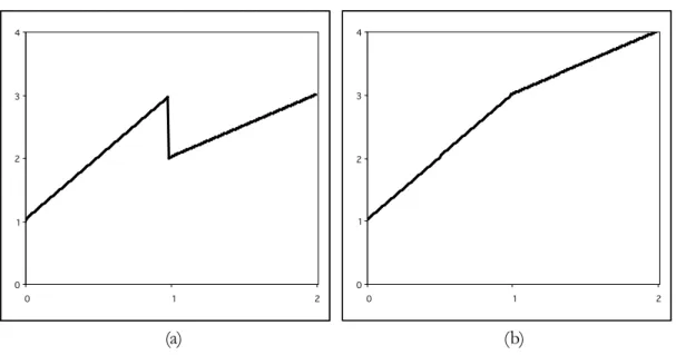
Unfortunately, the results of Easterly and Fischer’s study are faulty because their equation is faulty. By allowing the slope coefficients d1 through d4 to vary across decades while holding the intercept d0 fixed, Easterly and Fischer allow changes in the rate of growth of technology to become confused with changes in the level of technology. In particular, any decline in the rate of growth of technol-ogy between decades must necessarily be accompanied by a sudden decline in the level of technology.
⎩ ⎨ ⎧ ≥ + < + = ,1 1 1 2 1 x x x x y
while in panel (b), we have
⎩ ⎨ ⎧ ≥ + < + = . 1 2 1 2 1 x x x x y
Figure 1: Two Piecewise Linear Functions
0 1 2 3 4
0 1 2
0 1 2 3 4
0 1 2
(b) (a)
The function graphed in (a) drops discontinuously when the slope decreases, whereas the function graphed in (b) does not. The example is banal, but it makes the point: If one wants to write down an equation for a continuous piecewise lin-ear trend, one needs to allow the intercept term to vary along with the slope term. Easterly and Fischer’s specification of the log-technology process is of the kind shown in panel (a). This is a serious deficiency because, if the data does not sup-port a sudden decline in the level of technology at the end of each decade,5 then
estimated parameters will be less likely to reflect a decline in the rate of growth of technology, even if such a decline does match the data well. It seems safe to assume that this was not Easterly and Fischer’s intention.
A more appropriate specification for the production function, presumably
5 Using the CIA total economy data, a Wald test of the hypothesis that the intercept term in equation (1) is constant, versus the alternative hypothesis of an intercept that may vary between decades, yields a p-value of less than 0.01.
brenDan K. beare
consistent with the intended model of Easterly and Fischer, is
Here, D50-59 represents a dummy variable that is equal to one during 1950-59 and zero during other years. The other dummy variables are also defined in the obvi-ous way. This specification allows for a technology process with a rate of growth that varies across decades, but without inducing a sudden change in level. In other words, it is of the kind shown in panel (b) of Figure 1. Estimating equation (2) with the data used by Easterly and Fischer gives results very different from those obtained by estimating equation (1). These results are presented in the columns labeled CIA, KHA and OFF in Table 1. The three columns refer respectively to the CIA total economy data, the Khanin material sector data, and the official material sector data. Again, the estimates are obtained by employing a grid search over the nonlinear parameters g and a.
Let us first compare the results in columns EF and CIA, as these columns correspond to the estimation of equations (1) and (2) respectively, using the same data. The most obvious difference between the two sets of results is that the esti-mated standard errors are far larger in the latter. The estiesti-mated standard error on the elasticity of substitution using equation (2) is so large that we can say almost nothing about the magnitude of this parameter with any confidence. The esti-mates for d1 through d4 are more interesting, and suggest a monotone decline in the rate of technical change. The Wald statistic corresponding to the hypothesis d1 = d2 = d3 = d4has a p-value of 0.03, and so the hypothesis of a constant rate of technical change can be rejected at the 5% significance level.
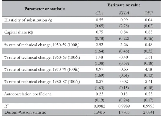
The Durbin-Watson statistic corresponding to the results in column CIA of Table 1 is 1.57. This number is neither high enough nor low enough for us to be clear about whether serial correlation in the residuals presents a serious prob-lem. Column CIA in Table 2 presents the results that were obtained when the production function was re-estimated with a correction for first order autocor-relation in the residuals, again using the CIA total economy data. Estimation for this column, and for the other columns of Table 2, was performed using a grid search over g, a, and the autocorrelation coefficient. The results in column CIA are generally similar to those obtained without correcting for autocorrelation, but the estimated standard errors are even larger. None of the estimated parameters are statistically significant. The Wald statistic corresponding to the hypothesis d1 = d2 = d3 = d4 now has a p-value of 0.096. In sum, the data tells us almost
noth-ing other than that the rate of technical change appears to be declinnoth-ing over the sample period.
( )
(
)
( )[
1]
.Table 2: Parameter Estimates for the Soviet Production Function, 1950-1987, Using a First-order Correction for Autocorrelation
Parameter or statistic Estimate or value
CIA KHA OFF
Elasticity of substitution (g) 0.55 0.99 0.04
(0.65) (2.78) (0.02)
Capital share (a) 0.75 0.84 0.85
(0.78) (0.22) (0.16) % rate of technical change, 1950-59 (100d1) 2.52 2.26 0.48
(1.64) (0.46) (0.32) % rate of technical change, 1960-69 (100d2) 1.48 -0.40 5.61
(1.08) (0.59) (0.18) % rate of technical change, 1970-79 (100d3) 0.97 -0.53 4.18
(1.69) (0.51) (0.13) % rate of technical change, 1980-87 (100d4) 0.27 0.02 2.61
(1.63) (0.15) (0.18)
Autocorrelation coefficient 0.23 0.18 0.25
(0.19) (0.24) (0.17)
R2 0.9982 0.9989 0.9995
Durbin-Watson statistic 1.9413 1.7705 2.0741
Note: Estimated standard errors in parentheses. CIA, KHA, OFF defined as in Table 1.
Next, consider the results obtained when we estimate equation (2) using the Khanin material sector data. These results are given in column KHA of Table 1 when we do not correct for autocorrelation, and column KHA of Table 2 when we do. In Table 1, the estimated elasticity of substitution is 0.99, with a standard error of 2.20. This is for a parameter that is expected to be between zero and one. When we correct for autocorrelation—the Durbin-Watson statistic is again ambiguous—the estimated elasticity remains at 0.99, and the standard error in-creases to 2.78. Essentially, given the model we are estimating, Khanin’s data tell us close to nothing about the elasticity of substitution. They do tell us that the rate of technical change appears to be significantly higher in the 1950s than in subsequent decades. The null hypothesis of a constant rate of technical change can be rejected using a Wald test at any reasonable significance level, whether or not we correct for autocorrelation.
brenDan K. beare
estimated elasticity of substitution is 0.04, with a standard error of only 0.02. The estimated rate of technical change is low in the 1950’s, increasing sharply in the 1960’s, and then declining over the remainder of the sample. A constant rate of technical change can easily be rejected at any reasonable significance level. The extremely low estimate of the elasticity of substitution using the official material sector data is surprising, especially in view of the results obtained using the other data sets. It is worth bearing in mind that, as noted by Easterly and Fischer, the official Soviet data for this sample period are widely believed to be misreported.
I have not reported estimation results based on the CIA or official data at the industry level because they suffer from an acute autocorrelation problem: with both datasets, the Durbin-Watson statistic is less than 0.52. Further analysis sug-gests that the residual process for equation (2) using the industry-level datasets may lack mean reversion.
The results we have reported in the CIA, KHA and OFF columns of Table 1 and Table 2 reveal very little about the nature of the Soviet economy during the sample period. There is evidence that the rate of technical change was declining over the sample period, but we can say almost nothing about the elasticity of sub-stitution or capital share parameters. The standard errors, and the discrepancies between data sets, are simply too large. This should not be surprising. Even if we ignore the poor quality of available data, estimation of a nonlinear model such as (2) using only thirty-eight observations, with a trend term that changes slope every ten periods, would seem to be extremely ambitious.
The apparent support provided to the extensive growth hypothesis by the results reported by Easterly and Fischer is clearly nothing more than an artifact of their inappropriate trend specification. What is surprising is that the defect in Easterly and Fischer’s analysis has not been noted previously. It has been more than a decade since the paper in question appeared in the World Bank Economic Review. As of January 2008, a search of the Social Sciences Citation Index yields 41 citations of the paper (including the working paper versions). None of those 41 papers note the error. Many refer specifically to Easterly and Fischer’s claim that the elasticity of substitution between capital and labor in the Soviet economy was significantly below one.
in Figure 1 is trivial; the problem with Easterly and Fischer’s trend specification would be obvious to anyone attempting to reproduce their results, or even just taking a careful look at equation (6) in their paper. It would seem that, despite the public accessibility of Easterly and Fischer’s data, no researcher has felt the need to take a closer look at the striking empirical results reported in their study.
referenceS
Easterly, William, and Stanley Fischer. 1994a. The Soviet Economic Decline: Historical and Republican Data. Policy Research Working Paper Series No. 1284. Washington: World Bank.
Easterly, William and Stanley Fischer. 1994b. The Soviet Economic Decline: Historical and Republican Data. NBER Working Paper No. 4735. Cam-bridge, MA: National Bureau of Economic Research.
Easterly, William and Stanley Fischer. 1995. The Soviet Economic Decline. World Bank Economic Review 9(3): 341-371.
Gomulka, Stanislaw and Mark Schaffer. 1991. A New Method of Long-Run Growth Accounting, with Application to the Soviet Economy 1928-87 and the US Economy 1949-78. Center for Economic Performance Discussion Paper No. 14. London: London School of Economics and Political Science. McCullough, B. D. 2007. Got Replicability? The Journal of Money, Credit, and
Banking Archive. Econ Journal Watch 4(3): 326-337. Link.
McCullough, B. D., Kerry Anne McGeary and Teresa Harrison. 2006. Lessons from the JMCB archive. Journal of Money, Credit and Banking 38(4): 1093-1107.
McCullough, B. D. and H. D. Vinod. 2003. Comment: Econometrics and Software. Journal of Economic Perspectives 17(1): 223-224.
brenDan K. beare
aBoutthe author
Brendan Beare is a Postdoctoral Prize Research Fellow
at Nuffield College, University of Oxford. He received his Ph.D. from Yale University in 2007. His primary field of re -search is econometric theory. His email is brendan.beare@
nuffield.ox.ac.uk.
Go to reply by Easterly and Fischer
Go to May 2008 Table of Contents with links to article
s
W
illiamE
astErly1ands
tanlEyF
ischEr2a rEply to: brenDan K. beare, “the Soviet economic Decline reviSiteD,” Econ Journal Watch 5(2), may 2008: 135-144. Link
abStract
WEarE gratEFul to BEarE (2008) For thEvaluaBlE sErvicE oF rE -checking our old results (Easterly and Fischer 1995). Beare’s main point is correct: we made a careless error in constraining the intercept of the time trend to be
con-stant while allowing trend coefficients to vary across decades. The consequence of this constant intercept assumption was not that our estimated equation produced
crazy jumps at the end of each decade, as Beare’s Figure 1 might be taken to imply.
It was instead that we biased the trend coefficients to be equal across decades (as Beare recognizes soon after Figure 1). So we gave biased support to our story that the slowdown in Soviet growth was not because of slowing TFP growth but rather was because of the extensive growth strategy of reliance on capital accumulation with a sharply falling rate of return to capital caused by a very low elasticity of
substitution between capital and labor.
Of course, while we failed to do a fair test of the assumption of constant
TFP growth, the assumption could still be correct. Our parsimonious model of a nearly constant TFP growth rate and low elasticity of substitution DID fit the data very well with sensible parameter values (except perhaps for our very high capital share, although even that could reflect a situation of initial surplus labor in
a non-market economy).
Unfortunately, the corrected model provided by Beare does not provide a very clear verdict on whether our story was correct or not. It would be desirable to relax
1 Professor of Economics, New York University. New York, NY 10012. 2 Governor, Bank of Israel. Jerusalem, Israel 91007.
We are grateful to Tobias Pfutze for diligent and thoughtful research assistance.
Reply to Brendan Beare
eaSterly & FiScher
our rigid assumptions so as to be able to test the alternative hypothesis of fluctuating and/or declining TFP growth and a higher elasticity of substitution in a completely unconstrained model. However, as Beare implicitly notes, it may be overly ambitious to estimate a fully flexible spline regression over time combined with a nonlinear function of capital with only 38 observations, which may not provide enough infor -mation content to allow sharp nested tests in a completely unconstrained model.
Indeed, in Beare’s piecewise continuous time trend using the CIA data, he
finds that he can reject that TFP growth rate is equal across decades, but he can -not reject that the capital share is zero, and he can-not pin down the elasticity of
substitution anywhere between zero and one. Beare’s 95% confidence interval for the capital share is {-0.724, 1.824} and that for the elasticity of substitution is {-0.7788, 2.2788}. In his results, we do not know whether capital has a positive (or negative) effect on output in any time period, whether capital and labor have zero substitutability or such high substitutability that labor is not even necessary in the long run (the latter would have made extensive growth very feasible). Hence, Beare is not able to go from his finding of decelerating TFP growth to also refute
our story that stressed the low elasticity of substitution and sharply declining
mar-ginal product of capital as the downfall of the extensive growth strategy.
We tried a more parsimonious specification of the TFP trend which turned
out to allow us to still precisely estimate the capital share and the elasticity of
substitution. This was simply specifying a quadratic function of time for the TFP element. The results were as follows:
Model with Trend and Squared Trend: ln(Y)=C1+C2*T+C3*T^2+gamma/(gamma-1)*ln(alpha*K^(gamma-1)/gamma+(1-alpha))
Parameter Estimate T-Stat
C1 -0.3844 -4.11
C2 0.0243 3.08
C3 -0.0003 -2.85
alpha (capital share) 0.83 11.45
gamma (elasticity of substitution) 0.49 7.56
The coefficient on the squared trend is significant and negative, indicat
-ing that we were wrong on constant TFP growth—TFP growth did decelerate.3
Since this exercise was inspired by Beare’s criticism, we are grateful to Beare for
correcting the part of the story that implied constant TFP growth. However, the elasticity of substitution is still very low, indicating that there were also sharply di
minishing returns to capital accumulation under “extensive growth”. This affirms our main point—the Soviet growth collapse was due in part to a rigid economy
that did not allow much substitution of labor with capital. As labor scarcities
de-veloped, the extensive growth strategy was doomed.
In addition, Beare's comment leads to the further conclusion that the rate
of technical progress declined over the course of the history of the former Soviet Union—a result that we regard as very plausible, and which we thank Beare for
pointing out as also being implied by the data.
rEFErEncEs
Beare, Brendan K. 2008. The Soviet Economic Decline Revisited. Econ Journal Watch 5(2): 134-144. Link.
Easterly, William and Stanley Fischer. 1995. The Soviet Economic Decline.
World Bank Economic Review 9(3): 341-371.
aBoutthE authors
William Easterly is Professor of Economics at New York University. His email address is [email protected].
Stanley Fischer is Governor of the Bank of Israel.
Go to Beare’s Comment
Go to May 2008 Table of Contents with links to article
s
Douglas Walker
Douglas M. Walker
1a rejoinDer To: earl l. grinols anD DaviD B. MustarD, “correctly critiqu-ing casino-criMe causality,” Econ Journal Watch 5(1), January 2008: 21-31.
link.
aBstract
i appreciaTeThaT professors grinols anD MusTarD (2008) replieD to my comment (Walker 2008). They say that, since I did not present empirical evidence for the “potential problems” I raised, they have no reason to alter their initial conclusions about the relationship between casinos and crime (30).
But if A estimates some effect, and B shows that the estimation is based on bad formulations and iffy data, it is rather irrelevant for A to respond: “But B hasn’t shown that reality is something other than my estimates.” My criticism wasn’t based on the claim that I know what the crime effects of casinos are; it was based on the demonstration that Grinols and Mustard have not given credible grounds for claiming that they know what the crime effects are.
I wish to revisit the crime rate issue as it pertains to the cost of casino crime estimates. I will also discuss the public consumption of research results.
The shifTfroM criMe raTeTo cosT BurDenper person
Consider Tunica County, Mississippi. The county population is around 10,000, and the county has 15 million visitors each year.2 Suppose there were
1,000 Index I crimes reported during a particular year. If we include the visitors
1 Department of Economics and Finance, College of Charleston. Charleston, SC 29424.
2 The 2005 estimated population was 10,321 (www.census.gov). The tourism estimate is from the Tunica Chamber of Commerce (www.tunicachamber.com).
The Diluted Economics of Casinos and Crime:
A Rejoinder to Grinols and Mustard’s Reply
Econ Journal Watch, Volume 5, Number 2, May 2008, pp 148-155.
in the denominator, then the crime rate is 0.000067; if not, it is 0.10.
Grinols and Mustard label the first the “diluted’ crime rate and the second “undiluted.” In the Tunica case, the “undiluted” crime rate is 1493 times greater than the “diluted” rate. To the extent that the Grinols and Mustard results depend on similar counties with a large ratio of tourists to residents, the exclusion of visi-tors from the population measure will have a real impact on the estimated crime rates. Clearly, one’s estimated cost of crime will change massively depending on whether one uses 0.000067 or 0.10 as the crime rate. Yet, Grinols and Mustard argue that differences in crime rate measures are not the central issue because the rate used depends on “what the researcher wants to do” (Grinols and Mustard 2008, 23).
In my comment, I had interpreted Grinols and Mustard’s purpose as esti-mating the change in the probability of casino county residents falling victim to crime with the introduction of casinos. My reason was that most of Grinols and Mustard’s justification for using the “undiluted” crime rate focused on showing that the “diluted” rate can fall even if the probability that a resident falls victim to crime increases. In their 2006 Review of Economics and Statistics article they write:
Should the number of crimes be divided by population—the con-ventional way to generate the crime rate (undiluted)—or by popula-tion plus visitors (diluted)?... Some have argued for one combinapopula-tion or another without realizing that the choice is not methodological, but depends on what questions the researcher wants to answer. A common but invalid claim is that the diluted crime rate should be used to determine the change in probability that a resident would be the victim of a crime. However, knowing what happens to the diluted crime rate does not give the needed information and could even move the answer in the wrong direction… (Grinols and Mus-tard 2006, 34)
Grinols and Mustard then give a lengthy, flawed example (discussed in Walker 2008, 8), and continue, “Thus, in this case the diluted crime rate falls while the probability of a resident being victimized rises” (Grinols and Mustard 2006, 35).
Grinols and Mustard (2008, 22) reply that my interpretation is wrong. They say they are not estimating the change in the probability of casino county residents falling victim to crime. They quote from their 2006 paper: “In this study we are interested in the costs to the host county associated with a change in crime from whatever source. We are therefore interested in the total effect of casinos on crime, and thus use the
undiluted crime rate….”3 And then immediately add: “In other words because crime
perpetrated in a given geographical area can impose costs that fall on local taxpayers,
Douglas Walker
it is appropriate to consider the total number of crime incidents relative to the local population and tax base” (Grinols and Mustard 2008, 22).
So they want us to focus on the costs of crime to casino hosting counties, rather than the risk to residents of falling victim to crime. Yet, the estimated cost of casino crime on casino hosting counties will be overstated if the crime rate attributed to county residents is overstated, as it is using their “undiluted” rate. If Grinols and Mus-tard want us to think in terms of cost burden per resident, they might elude the crime rate criticism, but the basis for that criticism simply re-emerges in terms of cost burden per resident.4
cosTsofcriMe
Grinols and Mustard estimate the casino crime cost burden to be $75 per adult casino county resident per year.5 This figure is emphasized in their abstract
(2006, 28) and it is the basis of their brief policy discussion (41-42). But does this figure actually mean what Grinols and Mustard say it means? No. As I pointed out in my original comment, Grinols and Mustard have implicitly attributed the entire cost burden to the residents—even if they are not victims of crimes! That is why I said their story would only make sense if all crimes are committed against casino county residents, and none against visitors (Walker 2008, 9-10).6
Grinols and Mustard use estimates of the cost per crime from Miller, Co-hen, and Wiersema (1996, 24) in order to estimate the cost of casino crime per casino county adult resident ($75). Yet, Miller et al. (1996) emphasize, “this study focuses on victims’ costs” (9) and “deliberately excludes two of the largest costs associated with crime—the cost of operating the criminal justice system and the cost of actions taken to reduce the risk of becoming a crime victim” (17). In fact, most of the estimated costs of crime are intangible costs such as lost quality of life, fear, pain, and suffering (21), that are borne by the crime victims—not by the taxpay-ers in the counties in which the crimes are perpetrated.7
Miller et al. (1996, 24, Table 9) estimate the cost of each robbery, for ex-ample, at $13,000. Of that amount, $10,700 is intangible costs. Grinols and Mus-tard’s failure to distinguish between resident and visitor victimizations effectively assumes that all costs—including intangible costs borne by casino county visitors
4 Rhetoricians might say that Grinols and Mustard’s argument for using the “undiluted” rate is an ipse-dixitism.
5 They write, “We use cost per victimization figures…to calculate the total social cost of crimes com -mitted in casino counties that are attributable to the presence of casinos…” (Grinols and Mustard 2006, 41). The abstract (28) indicates that these costs are on an annual basis. The details of the calculation are
not provided by Grinols and Mustard.
6 Grinols and Mustard attribute the costs to adult county residents—71% of the average county’s resi-dent population (Grinols and Mustard 2006, 41).
—fall on the residents. Otherwise it makes no sense for the “per person” part of the calculation to include only the county residents.
An analogy might help to confirm our understanding of what is going on. Let’s take an example that involves not costs per person, but benefits per person. The economic principle of mutual gains from voluntary interaction suggests that there are net benefits to those who voluntarily engage in sexual activity. What Grinols and Mustard have done is like saying that the sex benefits per person— that is, net benefits from sexual activity occurring within the county divided by the county population—is much higher in Carson City County, Nevada, than in practically all other counties in the country. But, in fact, the ordinary person who resides in Carson City County might in fact experience sexual benefits only about equal to or a little higher than ordinary residents in the other states. Benefits per person will appear artificially high if the numerous visitors to Carson City County are left out of the denominator. My suggesting that the residents should not open a casino because of the crime cost burden per person is $75 (as Grinols and Mustard estimate) would be analogous to suggesting that they should authorize brothels because their sex-benefit per person will go up significantly. But it is no more legiti -mate to encourage residents with the benefits of other people’s sexual experiences than it is to discourage them with costs of other people’s crime experiences.
It is certainly true that crimes impose some costs (policing, court, incar-ceration, etc.) on the county taxpayers, even when crimes are perpetrated against visitors. But Grinols and Mustard have not estimated that, since many of the costs that are borne by county taxpayers are explicitly ignored in the cost of crime esti-mates used by Grinols and Mustard (Miller et al. 1996, 17).
To summarize, most of the estimated cost of a crime against a visitor is not borne by residents—it is borne by that visitor. Furthermore, many of the costs that are borne by county residents and taxpayers are ignored in the cost of crime estimates used by Grinols and Mustard.8 Their $75 estimate of the cost of casino
crime per adult casino county resident is simply not meaningful.
puBlicconsuMpTionofgaMBlingresearch
If Grinols and Mustard’s estimates were ignored by the world, the dispute would be of merely scientific interest. But the results of Grinols and Mustard’s crime study (2006) have certainly had an influence on the public discourse on gambling. Professor Grinols was recently quoted in Parade Magazine (Flynn 2007) as saying that “if the damage [from gambling] were spread evenly among all of us, there’d be no gambling. Grinols also co-authored an op-ed (Grinols and Rose
Douglas Walker
2007) based on his other social cost research.
Professors Grinols and Mustard are frequently quoted in newspapers, on anti-gambling websites, and in academic debate over the social costs of casino anti-gambling.9 As a result, they have had, and will likely to continue to have, a significant impact on
the ongoing political debate in states like Kansas, Kentucky, and Massachusetts;10
and in other countries where casino legalization is under consideration. It is therefore worthwhile to examine some of the other “cost of gambling” figures that Grinols, in particular, often repeats to the media, in order to illustrate just how arbitrary are much of the publicized data on the economic effects of casinos.
Grinols and Mustard (2001, 154)11 and Grinols (2004, 171, 176) provide
estimates of the social costs of pathological gambling. They estimate costs at over $10,000 per pathological gambler, per year,12 and include a component for
the costs of crime. Based in part on this cost estimate, the authors argue that ca-sino gambling fails a cost-benefit test, with a ratio of 1.9:1 to 3:1, or even greater (Grinols and Mustard 2001, 155; Grinols 2004, 175-176).
Grinols has repeated these estimates in his op-ed on the effects of casinos (Grinols and Rose 2007), and has been quoted in the Wall Street Journal as saying that the introduction of a casino results in a net cost of over $97 per resident per year (Whitehouse 2007). In another newspaper article, Grinols was quoted, “I have concluded gambling as a whole is probably a bad idea for society” (Mona-han 2007). Mustard was quoted in the Washington Post as arguing that “even using conservative estimates of costs and generous estimates of benefits, we still find the costs exceed the benefits” (Morin 2006). More importantly, the Grinols and Mustard analysis served as an important component of a just-released Canadian study which its authors hope will be the new “gold standard” for social cost of gambling research.13
Clearly, Grinols and Mustard have been strong advocates in the public dis-course on casinos. Yet, the social cost estimate they provide is based on an av-erage of cost estimates from other studies. Most of those studies arrive at their
9 See Walker (2008, 4, note 2).
10 I recently received an unsolicited email by someone requesting my help: “I am on the vanguard of keeping casinos out of Kentucky and have written several articles over the last few years. The legislature is scheduled to bring a bill to amend the constitution soon. I was doing some research and ran across your piece, Do Casinos Cause Economic Growth… I gather from the abstract that your answer was a resounding ‘NO’. Is this what you concluded? I have had many discussions with Dr. John Kindt and also Dr. Earl Grinols, both of whom have helped me considerably in the past. I appreciate any ‘ammunition’ you can provide in this fight against this race to the bottom.”
11 Incidentally, Grinols and Mustard were the guest-editors of the issue of Managerial and Decision Eco-nomics in which their 2001 paper was published.
12 The costs attributable to pathological gamblers are widely regarded as being the major component of the costs of legalized casinos. However, these estimates by Grinols and Mustard depend on numerous very questionable assumptions.
estimates in ways highly arbitrary. Here are a few examples:14
In the study by Thompson, Gazel, and Rickman (1996, 19), the authors •
write, “The cost of probation and parole was estimated from the state budgets for corrections minus the costs of the operation of prisons, jails, and juvenile corrections. We assigned two-thirds of the residual budget to probation and parole costs, and divided the costs by the number of persons in these programs.”
Schwer, Thompson, and Nakamuro (2003, 15) explain how they calculated •
court costs: “[An earlier] study found that each federal court action costs $7,500. Considering that these actions may not be as complicated or long enduring as some others, we assign a 50 percent cost factor of $3,750 for each…case.”15 Focusing on money inflow and outflow to/from South Carolina as •
a representation of the benefits and costs of video gaming machines, Thompson and Quinn (1999, 10-12) explain, “There are 31,000 machines [in South Carolina]…They carry a [total] value of $46,500,000. The machines are for all intents and purposes manufactured out of state. We can assume that $46,500,000 leaves the state each year because of the machines.” Summing over all components, they conclude, “The money leaving the state…equals $133.3 million compared to $122 million coming into the state. In direct transactions, the state’s economy loses.”
These are only three examples, but they are sufficient to show just how arbi -trary such cost estimates are, both in methodological and empirical terms. Indeed, such studies have long been criticized for their poor quality, as discussed by the National Research Council (1999).16
conclusion
I do not fault Professors Grinols and Mustard for participating actively in the public discourse. I admire their vitality.17 But given the “potential problems” in
14 See Grinols and Mustard (2001, 153-154) and Grinols (2004, 172-174). Grinols and Mustard (2001, 152) acknowledge that only one of the eight studies on which they base their estimate was peer re-viewed.
15 Schwer et al. (2003) is cited by Grinols (2004) but obviously not by Grinols and Mustard (2001). For a discussion of other problems in the Schwer et al. (2003) analysis, see Walker (2007b, 628-637). 16 Walker and Barnett (1999) discuss many of these studies in detail, and the social costs of gambling in general. Problems in quantifying social costs are also addressed in Walker (2007a, 2007b).
Douglas Walker
their crime study, I do not believe strong conclusions about the costs of casino-related crime are justified. For any policy issue, researchers should acknowledge potential problems, and policy conclusions should be tempered accordingly. I agree with Grinols and Mustard that I do not have a good estimate of the cost of casino crime. But neither do they.
Perhaps more importantly, this is an excellent example of caveat emptor. Giv-en some of the examples of research discussed here, consumers of gambling re-search must be very careful to scrutinize the evidence—even when it is published in a reputable journal like Review of Economics and Statistics.
references
Flynn, S. 2007. Is gambling good for America? Parade Magazine. 20 May.
Grinols, E.L. 1997. Piety and political economy. Paper presented at the conference, “Christian Economists Doing Economics: A View from the Trenches.” Chicago,
IL.
Grinols, E.L. 2004. Gambling in America: Costs and Benefits. New York, NY: Cambridge University Press.
Grinols, E.L., and D.B. Mustard. 2001. Business profitability versus social profitabil -ity: Evaluating industries with externalities, the case of casinos. Managerial and Decision Economics 22: 143-163.
Grinols, E.L., and D.B. Mustard. 2006. Casinos, crime, and community costs. The Review of Economics and Statistics 88(1): 28-48.
Grinols, E.L., and D.B. Mustard. 2008. Correctly critiquing casino-crime causality. Econ Journal Watch 5(1): 21-31. Link.
Grinols, E.L., and J.S. Rose. 2007. Another voice: Laudatory report misstates conclu-sions on gambling. Buffalo News. 13 March.
Miller, T., M. Cohen, and B. Wiersema. 1996. Victim costs and consequences: A new look. U.S. Department of Justice.
Monahan, J. 2007. Economists fuel casino debate: Charges of bias leveled as barbs are traded. Worcester Telegram & Gazette. 28 Oct.
Morin, R. 2006. Casinos and crime: The luck runs out. Washington Post. 11 May. National Research Council. 1999. Pathological Gambling: A Critical Review. Washington,
DC: National Academy Press.
Schwer, K., W. Thompson, and D. Nakamuro. 2003. Beyond the limits of recre-ation: Social costs of gambling in Southern Nevada. Paper presented at the Far West and American Popular Culture Association Meeting. Las Vegas, NV. Socio-Economic Impact of Gambling (SEIG) Framework: An Assessment
Framework for Canada: In Search of the Gold Standard. Ontario Problem Gambling Research Centre. Link.
Thompson, W., R. Gazel, and D. Rickman. 1996. The social costs of gambling in Wisconsin. Wisconsin Policy Research Institute Report 9(6).
Thompson, W., and F. Quinn. 1999. An economic analysis of machine gambling in South Carolina. Report to the Educational Foundation. Columbia, SC: South Carolina Policy Council.
Walker, D.M. 2007a. The Economics of Casino Gambling. New York, NY: Springer. Walker, D.M. 2007b. Problems with quantifying the social costs and benefits of gam
-bling. American Journal of Economics and Sociology 66(3): 609-645.
Walker, D.M. 2008. Do casinos really cause crime? Econ Journal Watch 5(1): 4-20. Link. Walker, D.M., and A.H. Barnett. 1999. The social costs of gambling: An economic
perspective. Journal of Gambling Studies 15(3): 181-212. Whitehouse, M. 2007. Bad odds. Wall Street Journal. 11 June.
aBouTTheauThor
Douglas M. Walker is an associate professor of economics at the College of Charleston, in Charleston, SC. He received his Ph.D. in economics from Auburn University in 1998. Prior to coming to the College of Charleston, he taught at Auburn, Louisiana State University, and Georgia College. His research focus is on the economic and social effects of casinos and other types of legalized gambling. His book, The Economics of Casino Gambling, was published in 2007 by Springer. His gambling research has also been published in journals including American Journal of Economics and Sociolog y, Journal of Gambling Studies, Public Finance Review, and Review of Regional Studies. Here is a link to his website. His email is [email protected].
Grinols & Mustard
E
arll. G
rinols1andd
avidB. M
ustard2a rEply to: douGlas M. WalkEr, “thE dilutEd EconoMics of casinos and criME: a rEJoindErto Grinolsand Mustard,” Econ Journal Watch 5(2), May 2008: 148-155. link.
abstract
lEssthan onE Month followinGthE puBlication ofour dEtailEd
response to Professor Walker’s first commentary on our peer-reviewed work (Grinols and Mustard 2006), we were presented with a second manuscript by Mr. Walker (Walker 2008b). In his present commentary, Professor Walker again provides no new data or research, articulates comments that are already resolved through a careful reading of Grinols and Mustard (2006), and declines to respond to the failings that we raised about his earlier critique. In his second endeavor he also introduces new issues that were not in his first commentary note (Walker 2008a), expands his attention to the work of other authors, and makes factu-ally incorrect statements about their work. Because Mr. Walker’s complaints stem from errors of fact, correcting some of them might benefit future readers. We limit ourselves to four.
1. Mr. Walker says that our paper gives a “flawed example.” Mr. Walker is incorrect. The model presented in the original paper is a system of three equa-tions.
c = s1 + s2 + (σ1 + σ2)V/P
1 Department of Economics, School of Business, Baylor University. Waco, Texas 76798.
2 Department of Economics, Terry College of Business, University of Georgia. Athens, GA 30602.
Connecting Casinos and Crime:
More Corrections of Walker
D = (s1 + s2) P + VP + (σ1 + σ2) P + VV
p =s1 +s2
wherecis the crime rate, Ddefines the diluted crime rate,Pis the resident popula-tion, Vis the visitor population,s1 andσ1 are the shares of the resident and visitor population, respectively, victimized by residents, ands2 andσ2 are the shares of the resident and visitor population, respectively, victimized by visitors. p is the probability that a resident will be victimized. The purpose of the model is to show that the diluted crime rate (number of crimes divided by local population + visi-tors) can fall while the probability of a resident being victimized rises (i.e.p and
Dcan move in opposite directions.) For example, assume as in the paper thatσ1
= 0.Lets1 = 0.10.In the no visitor situation V= s2=σ2= 0 andp =D=0.10. Now let visitors be present,V=P=1000, wheres2=σ2=0.04. As we originally showed, thenprises (from 0.10 to 0.14) whileDfalls (from 0.10 to 0.04). There is an infinite number of other ways the same result may occur.
2. Mr. Walker also expands his criticisms beyond Grinols and Mustard (2006) to papers written by other authors (Thompson, Gazel, Rickman 1996b; Thompson and Quinn 1999; and Schwer, Thompson, and Nakamuro, 2003). This is consistent with his pattern of writing “rebuttals” in which he provides no origi-nal research or no new empirical work.3 In his present commentary, Mr. Walker
also misinterprets or misunderstands the work of other researchers. He writes:
These are only three examples, but they are sufficient to show just how arbitrary such cost estimates are, both in methodological and empirical terms. Indeed, such studies have long been criticized for their poor quality, as discussed by the National Research Council
3 In 1998 he produced a rebuttal of Gross (1998) that provided no original research or empirical work. A few years later he wrote a rebuttal of Kindt (2001), which criticized the gambling industry and
Grinols & Mustard
(1999). (Walker 2008b, 153)
Two of the three studies Mr. Walker cites are, in fact, not cited by the Na-tional Research Council (NRC) report. One of these papers could not possibly have been cited in NRC (1999) because it was written four years after the report was published. Furthermore, Thompson, Gazel, and Rickman (1996b) was cited
favorably, not critically, by the NRC.4The NRC refers to the study as “an excellent
example” and a study that “makes a significant contribution to the literature on the economic impacts of gambling.”
3. In the same section, Walker cites Grinols (2004) in his footnote 14, in-serted after the sentences “Most of these studies arrive at their estimations in ways highly arbitrary. Here are a few examples.” As shown above, the basis for much of Mr. Walker’s perspective is misreading of the original papers. Walker (2007), written for the American Gaming Association, the chief lobbying body of the gambling industry, discusses the need for gambling research to adjust for co-morbidity (multi-causality). He writes that “a mechanism is needed to allocate the harm among coexisting disorders, yet most authors make no such attempt.” He states: “Most social cost researchers (e.g., Grinols 2004, Grinols and Mustard 2001, and Thompson et al. 1997) simply attribute all of the costs to gambling.” This statement, too, is false. Page 173 of Grinols 2004 states that the reported cost figures were adjusted by the author to correct for multi-causality, as well as for a second issue, sample selection bias (representativeness of sample). Both are explained in detail on pp. 170-71.
4. Mr. Walker devotes nearly four manuscript pages to his view of how
4 Thompson, Gazel, Rickman 1996b is cited four times by NRC. They are singled out positively on page 173:
An excellent example of this type of analysis is a study that looked at the economic ef-fects that casinos have had in Illinois and Wisconsin (Thompson et al., 1996b)….The result was a set of estimates of the positive and negative monetary effects of casino gambling in both Illinois and Wisconsin. This, in turn, provided a good estimate of the positive effects of casinos in the two states….
The three other citations are simple references to earlier results as on page 28:
Studies primarily of gamblers seeking help suggest that as many as 20 percent will at-tempt suicide (Moran, 1969; Livingston, 1974; Custer and Custer, 1978; McCormick et al., 1984; Lesieur and Blume, 1991; Thompson et al., 1996), and two out of three help seekers have turned to criminal activities to support their gambling (Lesieur et al., 1986; Brown, 1987; Lesieur, 1989).
NRC also reports favorably on Thompson, Gazel, Rickman 1996a on page 181:
A second study that makes a significant contribution to the literature on the economic impacts of gambling is one that identifies and quantifies the social costs of gambling in the state of Wisconsin (Thompson et al., 1996a).
crime statistics should be measured. As stated in our previous response, we ad-dressed this issue extensively in the original paper and encourage readers to re-turn to our original paper. In Mr. Walker’s initial commentary, he objected to our using conventional, federally-reported crime rates in our study. His position has now evolved. In his earlier commentary he said,
the apparent objective of the Grinols and Mustard paper is to an-alyze the risk of casino county residents falling victim to crime. (Walker 2008a, 7)
and
In this case, clearly the ‘diluted’ crime rate is the appropriate one to use if we are trying to measure the risk to residents and/or visitors of being victimized. (Walker 2008a, 10)
His previous concern was based on an incorrect reading of the paper. Our paper states, “We are therefore interested in the total effect of casinos on crime” (Grinols and Mustard, 30, emphasis added) as “Correctly Critiquing Casino-Crime Causal-ity” further confirmed.
His original comment resolved, Mr. Walker now shifts his focus to crime costs. In his new comment he says, “they might elude the crime rate criticism, but the basis for that criticism simply re-emerges in terms of cost burden per resident.” He says,
Grinols and Mustard have implicitly attributed the entire cost bur-den to resibur-dents—even if they are not victims of crimes! (Walker 2008b, 150)
This also is false. We have not “implicitly attributed the entire cost burden to residents” as Mr. Walker erroneously claims. In fact we explicitly said the op-posite. In the section titled “Visitor Criminality,” we said that crime could rise “because casinos attract visitors who are more prone to commit and be victims of crime”
(Grinols and Mustard 2006, 32, emphasis added). Earlier in the paper we pro-vided theoretical explanations of how casinos might affect crime. We said, “These factors are not mutually exclusive, and our empirical results estimate the total effect” (emphasis added). That crime might increase in casino counties because visitors were crime victims was repeated again on page 40 in our section labeled “Evalu-ation” where we wrote, “The regressions in table 4, of course, cannot decompose the net number of offenses to assign them to each alternative explanation.”
Grinols & Mustard
calculating the estimated costs we deliberately chose results that provided smaller estimates of the casino effects than did some of our other specifications.
Concerning the denominator, the social costs associated with increased crime involves the change in absolute number of crime incidents. The divisor used in the initial reporting of crime (whether population or population + visi-tors) disappears before the final step, hence is irrelevant. In the portion of the paper detailing costs, the paper reports:
In 1996 the total costs for the 178 casino counties exceeded $1.24 billion per year. (Grinols and Mustard 2006, 41)
What would the costs be if they were extrapolated to the U.S.? The next sentence reads:
If the estimated coefficients from table 4 are applied to a represen-tative county of 100,000 population, 71.3% of which are adults (as is representative of the United States as a whole), then the social costs per adult are $75 in 2003 dollars.
The answer is $75 per adult, as reported.
In conclusion, many papers, Grinols and Mustard 2006 included, describe areas where further research could improve on earlier contributions. Indeed, this is the theme of much, if not most, academic research in the social sciences. When we saw the need for better research on the statistical link between casinos and crime we researched, wrote, and published Grinols and Mustard (2006). Unless better research comes along to confirm or deny our peer-reviewed results, we stand by our conclusions.
rEfErEncEs
Benston, Liz. 2003. Expert: Problem Gambling Study Flawed. Las Vegas Sun. 31 March 2003.
Grinols, Earl L. and David B. Mustard. 2006. Casinos, Crime, and Commu-nity Costs. The Review of Economics and Statistics 88(1): 28-45.
Grinols, E.L., and D.B. Mustard. 2008. Correctly critiquing casino-crime causality. Econ Journal Watch 5(1): 21-31. Link.
Grinols, Earl L. 2004. Gambling in America: Costs and Benefits. New York: Cam-bridge University Press.
Economic Development Quarterly 12(3): 203-213.
Kindt, John. 2001. The Costs of Addicted Gamblers: Should the States Initi-ate Mega-Lawsuits Similar to the Tobacco Case? Managerial and Decision Economics 25(4): 197-200.
National Research Council. 1999. Pathological Gambling: A Critical Review. Wash-ington, DC: National Academy Press.
Policy Analytics. 2006. A Benefit-Cost Analysis of Indiana’s Riverboat Casi-nos for FY 2005, 17 January. Unpublished.
Schwer, R. Keith, William N. Thompson, Daryl Nakamuro. 2003. Beyond the Limits of Recreations: Social Costs of Gambling in Southern Nevada. 2003 Annual Meeting of the Far West and American Popular Culture As-sociation, Las Vegas, NV, February 1, 2003. Revised: February 18, 2003. Revised May 28, 2003 as Thompson, William N. and R. Keith Schwer. Beyond the Limits of Recreation: Social Costs of Gambling in Southern Nevada. 14th International Conference of Gambling and Risk Taking, Fairmont Waterfront Hotel, Vancouver, British Columbia, May 28, 2003.
Thompson, W.N., R. Gazel, and D. Rickman. 1996a. Casinos and Crime in Wisconsin: What’s the Connection? Thiensville: Wisconsin Policy Research Institute Inc.
Thompson, W.N., R. Gazel, and D. Rickman. 1996b. The Social Costs of Gam-bling in Wisconsin. Thiensville: Wisconsin Policy Research Institute Report, Vol. 9, No. 6.
Walker, Douglas M. 2007. Challenges that Confront Researchers on Estimat-ing the Social Costs of GamblEstimat-ing. Prepared for the American GamEstimat-ing Association.
Walker, D.M. 2008a. Do Casinos Really Cause Crime? Econ Journal Watch 5(1): 4-20. Link
Grinols & Mustard
aBoutthE authors
Earl L. Grinols is Distinguished Professor of Economics at the Hankamer School of Business at Baylor University and former Senior Economist for the Council of Econom-ic Advisers. A University of MEconom-ichigan Angell Scholar and mathematics summa cum laude graduate of the University of Minnesota, he earned his PhD at MIT. In addition to Baylor, he has taught at MIT, Cornell University, the University of Chicago, and the University of Illinois. His current research focus, health care, is treated in his book Health Care for Us All: Getting More for Our Investment (Cambridge University Press, forthcoming) co-authored with colleague James W. Henderson.
David B. Mustard is an Associate Professor of Economics in the Terry College of Business at the University of Georgia and a research fellow at the Institute for the Study of Labor in Bonn, Germany. Mustard earned a Ph.D. in Economics from the University of Chicago. His research focuses on microeco-nomic policy-related questions, especially law and ecomicroeco-nomics, crime, casino gambling, lotteries, gun control, sentencing, la-bor economics, education and merit-based aid. Mustard has won many university- and college-wide teaching awards and regularly teaches in UGA’s honors program.
Go to Walker’s Original Article
Go to Grinols and Mustard’s Reply
Go to Walker’s Rejoinder
Go to May 2008 Table of Contents with links to article
s
DaviD R. HenDeRson
1a RejoinDeRto: Benjamin alamaR and stanton glantz, “smoking in Restau-Rants: a Reply to HendeRson,” Econ Journal Watch 4(3), septemBeR 2007: 292-295. link.
aBstRact
in tHeiR last paRagRapH, alamaR anD glantz (2007) wRite, “Hen -derson (2007) does not accurately identify any problems either theoretically or statistically with our analysis.” This is an amazing conclusion, given that I did identify theoretical and statistical problems with their analysis. I will respond to the specifics, but I invite the reader to read my article and their reply together. Alamar and Glantz (2007) have largely chosen to ignore my criticism. I close with
a challenge to Alamar and Glantz.
economic tHeoRy
A quick recounting of our theoretical differences, up to but not including their response, is in order. Alamar and Glantz (2004) assert that smoking in restau-rants imposes externalities. They argue that the large number of customers “with greatly varied preferences” with regard to smoking causes negotiation costs to be high. This, they argue, “violates the assumption of low costs in the Coase theorem” and, they conclude, makes smoking an externality that is not internalized.
My criticism (Henderson 2007) is that restaurant owners do not have to negotiate with customers. All they need do, whether the issue is smoking, dress-code policy, music, or menu choices, is make their decision and see how successful
1 Graduate School of Business and Public Policy, Naval Postgraduate School. Monterey, CA 93943. I thank Warren Gibson, Rena Henderson, and Michael Pakko for helpful comments.
Smoking in Restaurants: Rejoinder to Alamar
and Glantz
daVid R. HendeRson
they are. Customers who want to eat in a non-smoking restaurant can do so; cus-tomers who want to eat in a smoking restaurant can do so; cuscus-tomers who want to eat in a restaurant that allows smoking in a designated area can do so. Customers show their values of these various options by the prices they are willing to pay and by the frequency of their patronage. Restaurant owners have an unbiased incentive to trade off the values put on smoking by various potential patrons and, therefore, do not reach a biased result in favor of allowing smoking. Introducing the desires of restaurant employees complicates the analysis without changing the bottom line: restaurant owners have an incentive, via wages paid and workmen’s compensation, to take account of the desires of the employees also.
In their reply, Alamar and Glantz write:
It is not possible for a restaurant owner to internalize the cost of second-hand smoke on the health of the staff or patrons. There is no mechanism by which a restaurant owner can compensate a pa-tron for any health costs related to second-hand smoke, therefore it is not possible for the owner to have completely internalized the costs of the externality imposed by the smoker. (292)
Alamar and Glantz have completely missed my point. My argument is that not only is it possible for restaurant owners to internalize the cost, but also that that is what they do. There is no need for a “mechanism” to compensate a patron. Instead, the patron decides on the negative value he or she puts on a restaurant that has smoke and that negative value is reflected in what he or she is willing to pay for the restaurant experience. In that way, the putative externality is internal-ized. That is why I said that they beg the question: they start with the assumption that smoking in a restaurant imposes externalities rather than establishing that it does. It is not surprising that if one assumes that there is an externality, one will be driven to the conclusion that there is an externality. Interestingly, Alamar and Glantz (2007) avoided responding to my analogy between smoking policy and T-shirt policy. Yet all their reasoning, if correct, can be applied to T-T-shirt policy.
and expected features of experience you find in the restaurant.
Finally, Alamar and Glantz (2007) state, “Henderson (2007) claims that we do not put enough faith in these entrepreneurs’ views,” namely the view that if consumers value it highly enough, some entrepreneurs will gain from a smoke-free environment. But I said nothing about faith. Rather, I believe that entre-preneurs often experiment and that some entrepreneurial restaurant owners will experiment with a ban on smoking. Then if banning smoking is as good for the bottom line as Alamar and Glantz claim, they will stick with the ban. When other restaurant owners observe the results, then they too will be more inclined to ban smoking—if, that is, Alamar and Glantz are right about the profitability of instituting bans on smoking. This is the standard story about what happens in competitive markets. Where is the “faith” in this story? Indeed, it is Alamar and Glantz (2007) who have faith, in two ways. First, they assert, “When these entrepreneurs only have the biased information given to them from the tobacco industry (without being told that it is coming from the tobacco industry (Alamar and Glantz 2004)) how are they to know that the information is biased?” Um, maybe by getting other information? Alamar and Glantz have complete faith that the tobacco industry has been such a powerful persuader that they have made all restaurant owners completely uncurious. This view that the restaurant owners have considered no other information is a strange view and one for which they give zero evidence.
There’s another group in which Alamar and Glantz seem to have faith: voters. Basic public choice analysis has explored how enlightenment depends on incentives to overcome the costs and biases of ignorance, and on the complexity of the issues considered. Alamar and Glantz turn these teachings on their head. They show remarkably little confidence in the self-regarding wisdom of restaurant owners who have a huge amount at stake, and yet they have great confidence in the wisdom of voters, most of whom individually have little at stake. The exter-nality from smoking, Alamar and Glantz argue, “is one reason that the public has demanded laws to make restaurants smokefree.”
Yet, compared to restaurant owners, voters have much less incentive to become more enlightened in the matter, and the political issue they face as voters is vastly more complex than the decision a restaurant owner faces concerning his own particular business and his own customers. Somehow Alamar and Glantz overlook such elementary analysis.