Complex Systems Informatics and Modeling Quarterly (CSIMQ) eISSN: 2255-9922
Published online by RTU Press, https://csimq-journals.rtu.lv Article 113, Issue 19, June/July 2019, Pages 75–98
https://doi.org/10.7250/csimq.2019-19.05
A Methodology for Operationalizing Enterprise IT Architecture and
Evaluating its Modifiability
Robert Lagerström1*
, Alan MacCormack2, David Dreyfus3, and Carliss Baldwin2
1
Electrical Engineering and Computer Science, KTH Royal Institute of Technology, Stockholm, Sweden
2
Harvard Business School, Boston, USA 3
NorthBay Solutions, Boston, USA
[email protected], [email protected], [email protected], [email protected]
Abstract. Recent contributions to information systems theory suggest that the primary role of a firm’s information technology (IT) architecture is to facilitate, and therefore ensure the continued alignment of a firm’s IT investments with a constantly changing business environment. Despite the advances we lack robust methods with which to operationalize enterprise IT architecture, in a way that allows us to analyze performance, in terms of the ability to adapt and evolve over time. We develop a methodology for analyzing enterprise IT architecture based on “Design Structure Matrices” (DSMs), which capture the coupling between all components in the architecture. Our method addresses the limitations of prior work, in that it i) captures the architecture “in-use” as opposed to high level plans or conceptual models; ii) identifies discrete layers in the architecture associated with different technologies; iii) reveals the “flow of control” within the architecture; and iv) generates measures that can be used to analyze performance. We apply our methodology to a dataset from a large pharmaceutical firm. We show that measures of coupling derived from an IT architecture DSM predict IT modifiability – defined as the cost to change software applications. Specifically, applications that are tightly coupled cost significantly more to change.
Keywords: Enterprise Architecture, Modularity, Information Systems, Modifiability, Design Structure Matrix.
1
Introduction
As information becomes more pervasive in the economy, information systems within firms have become more complex. Initially, these systems were designed to automate back-office functions
*
Corresponding author
© 2019 Robert Lagerström et al. This is an open access article licensed under the Creative Commons Attribution License (http://creativecommons.org/licenses/by/4.0).
Reference: R. Lagerström, A. MacCormack, D. Dreyfus, and C. Baldwin, “A Methodology for Operationalizing Enterprise IT Architecture and Evaluating Enterprise IT Modifiability,” Complex Systems Informatics and Modeling Quarterly, CSIMQ, no. 19, pp. 75–98, 2019. Available: https://doi.org/10.7250/csimq.2019-19.05
76 and provide data to support managerial decision-making. Their role was expanded to coordinate the flow of production in factories and supply chains. The invention of the personal computer led to the creation of client-server systems, which enhanced the productivity of office workers and middle managers. Finally, the arrival of the Internet brought a need to support web-based communication, e-commerce, and online communities. Today, even a moderately sized business maintains information systems comprising hundreds of applications and databases, running on geographically distributed hardware platforms, and serving multiple clients. These systems must be secure, reliable, flexible, and capable of evolving to meet new challenges.
“Enterprise architecture” (EA) is the name given to a set of frameworks, processes and concepts used to manage an enterprise’s information system infrastructure. For instance, TOGAF®, the most-cited framework in this field, was developed by a consortium of firms to provide a standardized approach to the design and management of information systems within and across organizations [1]. It provides a way of visualizing, understanding and planning for the needs of diverse stakeholders in a seamless way. Despite the increasing adoption of EA frameworks by firms, however, the empirical evidence for their impact is mixed at best [2]–[8]. Making changes to systems, adding new functions, and/or integrating different systems (e.g. during a merger) continue to be difficult tasks. Changes made to one component often create unexpected disruptions in distant parts of a system [9]–[12]. In essence, when dealing with complex information systems, changes propagate in unexpected ways, increasing the costs of adaptation. This suggests that we need a better way to operationalize (and analyze) enterprise IT architecture.
Early contributions to the EA literature focused on the need to align IT investment decisions with the business strategy of a firm (e.g. [13]). With this perspective, a firm’s architecture should be optimized to a given strategic position, and was expected to change only slowly, as a firm evolved. Contributions to theory however, focus on the complex and dynamic nature of competition in today’s business markets, and the increasingly pervasive nature of digital platforms [14]–[16]. Given this, viewing the design of a firm’s enterprise architecture as a static optimization problem is no longer possible. Instead, modern information systems theory emphasizes the need for IT architectures to facilitate IT modifiability, through the use of modular, loosely coupled systems [17], [18]. Firms with superior modifiability quickly reconfigure resources to respond to new challenges, ensuring a continuous alignment of IT investments with changing business needs.
How can we operationalize the concept of enterprise IT architecture in a way that is robust, repeatable, and facilitates the analysis of IT modifiability? Prior work has demonstrated the efficacy of using a Design Structure Matrix or DSM – a square matrix that captures dependencies between components – as a tool for visualizing, measuring and characterizing product architecture [19]–[21]. We apply this methodology to analyze a firm’s enterprise IT architecture, which comprises many interdependent elements, including business groups, applications, databases and hardware. We use data from a large pharmaceutical company to i) describe how an enterprise IT architecture DSM is constructed, ii) show that this DSM reveals the layered structure of the architecture, and iii) highlight how this DSM allows components in the architecture to be classified into different groups – Core, Peripheral, Shared and Control – based upon the way that they interact with and are coupled to other components. We then analyze the impact of component coupling on IT modifiability – defined as the cost to change software applications. We show that the cost to change “Core” applications, which are tightly coupled to other components, are significantly higher than the cost to change “Peripheral” applications, which are only loosely connected to other components. The measure of coupling which best predicts IT modifiability is one that captures all direct and indirect connections between components. In sum, it is important to account for all possible paths by which changes may propagate between components in the architecture.
77 been applied to the study of product architecture, can be used to gain insight into enterprise IT architecture. We demonstrate the application of our methodology using a novel dataset from a real firm, encompassing comprehensive information about all system components and the interdependencies between them. We show that this method can be used to predict IT modifiability – the most critical capability in the modern firm. We conclude by relating our findings to the prior literature and discussing the implications of our methods for managerial practice.
The article is organized as follows. Section 2 reviews the literature and motivates our approach. Section 3 introduces our dataset and describes how an enterprise IT architecture DSM is constructed. Section 4 shows how this DSM is used to classify components into groups based upon their levels of coupling. Section 5 shows how measures of coupling derived from the DSM can be used to predict the cost of software changes. Finally, Section 6 describes our conclusions.
2
Literature Review
This section first reviews the enterprise architecture literature, with the aim of understanding the limitations of current approaches, and the criteria by which new methods should be assessed. We then describe work on the visualization and measurement of complex software systems using network-based approaches, with a focus on the use of DSMs.
2.1 Enterprise Architecture
Enterprise Architecture is commonly defined as a tool for achieving alignment between a firm’s business strategy and its IT infrastructure. For instance, MIT’s Center for Information Systems Research defines EA as “the organizing logic for business processes and IT infrastructure reflecting the integration and standardization requirements of the company's operating model” [13]. Prior work tends to emphasize conceptual models, tools and frameworks that attempt to achieve this alignment (e.g. [22]). EA analysis is not limited to IT systems, but encompasses the relationship with and support of business entities.
This overarching perspective is present in the ISO/IEC/IEEE 42010:2011 standard, which defines architecture as “the fundamental organization of a system, embodied in its components, their relationships to each other and the environment, and the principles governing its design and evolution” [23]. Ultimately, EA targets a holistic and unified scope of organization [24], [25]. Hence most research has focused on the “strategic” implications of EA efforts [26]–[29].
If the integration of IT and business concerns is one defining aspect of EA, a model-based methodology is another. As the name hints, architectural descriptions are central in EA. These descriptions include entities that cover a broad range of phenomena, such as organizational structure, business processes, software and data, and IT infrastructure [30]–[33]. A large number of frameworks have been proposed, detailing the entities and relationships between them that should be part of this effort (e.g. [1], [30], [34]). However, considerable diversity exists, in terms of the primary unit of analysis and terminology adopted by each. For instance, various frameworks focus on i) Stakeholders and Aspects to be considered [34]; ii) Viewpoints and Concerns to be analyzed [1]; and iii) Objects and Attributes to be modeled [35]. This lack of consistency is likely one reason for the limited success reported for EA efforts in studies of practice [36].
78 Several EA frameworks propose using matrices to display the relationships among various components of an information system, in an attempt to make EA more operational. For instance, TOGAF recommends preparing nine separate matrices at different points in the development of a firm’s architecture,†
which are used to track the linkages and dependencies between various parts of the system. Unfortunately, it is not clear how these matrices should be combined to generate managerial insights. Furthermore, the information used to construct them reflects an idealized view of how a system should function, rather than how it actually functions. Finally, these matrices do not yield quantitative measures of architecture that can be used to analyze performance, they are primarily descriptive in nature.
In sum, operationalizing enterprise architecture in a robust and reliable way, that allows firms to analyze and improve their systems, has proven an elusive goal. A diverse range of frameworks exists, each employing different units of analysis and terminology. Furthermore, these frameworks are conceptual in nature, generating few quantitative measures that can be used to analyze performance. Finally, these frameworks focus on idealized versions of a firm’s architecture, rather than actual data from the architecture “in-use.” While some studies attempt to operationalize EA at a granular level (e.g. [42], [43]), there is yet little consensus on a general methodology for how this should be achieved.
2.1.1 Enterprise Architecture and “Layers”
While there exists a diverse range of enterprise architecture frameworks, one of the themes they have in common is the concept of “layers” [44]–[46]. Simon et al. [44] describe enterprise architecture management as dealing with different layers, including business, information, application, and technology layers. Yoo et al. [45] argue that pervasive digitization has given birth to a “layered-modular” architecture, comprising devices, network technologies, services and content. Finally, Adomavicius et al. [46] discuss the concept of an IT “ecosystem,” highlighting the different roles played by products and applications, component technologies and infrastructure technologies.
While studies differ in the ways they classify layers in a firm’s enterprise architecture, they do share common underlying assumptions. First, layering reflects a division of the functions provided by a system into units, such that these units can be designed, developed, used and updated independently. Second, layering establishes a design “hierarchy” such that each layer tends to interact only with layers immediately above or below it, reducing complexity [47]. Finally, the direction of interdependencies between layers is such that higher layers “use” lower layers, but not the reverse, limiting the potential for changes to propagate [48]. For instance, a software application on a desktop computer “uses” (i.e. depends upon) functions provided by the operating system layer below it. However, the operating system does not (in general) depend upon the applications that use it. This has important implications for the propagation of changes. Changes to the operating system may impact applications, but changes to applications will not, in general, impact the operating system. The importance of layering in the literature suggests that any methodology for operationalizing EA should be able to identify the layered structure of the architecture.
2.1.2 Enterprise Architecture, Firm Performance and IT Modifiability
Much of the literature on EA has focused on frameworks that align business needs with IT capabilities and the processes by which such frameworks are implemented. Surprisingly, there has been little work to explore the performance benefits of EA, using empirical data on the actual outcomes achieved by firms [6]–[8]. Indeed, Tamm et al. [26] found that of the top 50 articles on enterprise architecture (as ranked by citation count) only 5 provided any empirical data that sought to explain the link between EA efforts and improved performance outcomes. Studies that do make claims about the performance benefits of EA tend to cite a range of “enablers” that mediate important firm outcomes. Recurring themes include better organizational
†
79 alignment, improved information quality and availability, optimized resource allocation across a business portfolio, and increased complementarities between firm resources [26].
Many authors note it is difficult to directly assess the quality of a firm’s architecture. Hence empirical studies linking enterprise architecture to performance tend to focus on assessing the quality of the outputs from EA planning processes (e.g. the quality of the documentation) or the quality of the planning process itself (e.g. how effectively did the firm set goals, define tasks and govern the effort) [49]–[52]. This approach means that it is difficult to differentiate between firms that follow similar EA planning processes, but which arrive at different system designs. A more robust method for operationalizing EA should be able to discern between such situations.
The most consistent theme that emerges in the literature is the increasingly important role of enterprise IT architecture in facilitating agility. In an influential paper, Samburmathy at al [53] argue that the strategic value of information technology investments in firms is defined by their impact on agility, creating “digital options” and improving “entrepreneurial alertness” (i.e. understanding and exploiting new opportunities). Sambamurthy and Zmud [54] suggest the new organizing logic for IT architecture is the “platform,” which encompasses a “flexible combination of resources, routines and structures” that meets the needs of both current and future IT-enabled functionalities. Duncan [55] and Schmidt and Buxmann [51] explore the factors that contribute to flexibility, and show managers associate this feature with the attributes of compatibility, connectivity, and modularity. Finally, Tiwana and Konsynski [17] use modular systems theory to develop subjective measures of IT architecture, and show that loose coupling and the use of standards are associated with self-reported increases in a firm’s level of IT agility.
The above discussion suggests that any methodology for operationalizing enterprise IT architecture in a more robust way must capture data on the architecture “in-use” by a firm, and not just the processes and documents by which it was developed. Furthermore, the measures output from this methodology should facilitate the analysis of IT agility (flexibility/modifiability), given the importance of this construct in the literature on the role of information systems in the modern firm.
2.2 Network-based Approaches to System Architecture
Many prior studies have characterized the architecture of complex systems using network representations and metrics [56]–[58]. In particular, they focus on identifying the linkages that exist between different elements (nodes) in a system [59], [60]. A key concept that emerges in this literature is that of modularity, which refers to the way that a system’s architecture can be decomposed into different parts. Although there are many definitions of modularity, authors agree on its fundamental features: the interdependence of decisions within modules, the independence of decisions between modules, and the hierarchical dependence of modules on components that embody standards and design rules [61], [62].
Studies that use network methods to measure modularity typically focus on analyzing the level of coupling between different elements in a system [63].‡ The use of graph theory and network measures to analyze coupling in software systems has a long history [65]. Many authors find measures of direct component coupling predict important parameters such as defects and productivity [66]–[70]. In more recent years, a number of studies have adopted coupling measures derived from social network theory to analyze software systems [43], [71], [72]. However, such measures suffer from limitations that make their application to technical systems difficult to apply and interpret. For instance, social network measures tend to assume that dependencies are symmetric. In technical systems, many important dependencies are asymmetric, meaning the direction of coupling is important.
‡
80 2.2.1 Design Structure Matrices (DSMs)
An increasingly popular network-based method used for analyzing technical systems is the “Design Structure Matrix” or DSM [19], [20], [73], [74]. A DSM displays the structure of a complex system using a square matrix, in which the rows and columns represent system elements, and the dependencies between elements are captured in off-diagonal cells. Baldwin et al. [75] show that DSMs can be used to visualize the “hidden structure” of software systems, by analyzing the level of coupling for each component, and classifying them into similar categories based upon the results.
Metrics that capture the level of coupling for each component can be calculated from a DSM and used to understand system structure. For instance, MacCormack et al. [20] and LaMantia et al. [76] use DSMs and the metric “propagation cost” to compare software system architectures, and to track the evolution of software systems over time. MacCormack et al. [77] show that the architecture of technical systems tends to “mirror” that of the organizations from which they have evolved. Sturtevant [78] shows that software components with high levels of coupling tend to experience more defects, take more time to adapt and are associated with high employee turnover. Ozkaya [79] shows that metrics derived from DSMs can be used to assess the value released by “re-factoring” designs with poor architectural properties. And Lagerström et al. [80] connects DSM-based complexity measures with known vulnerabilities in Google Chrome.
2.2.2 Design Structure Matrices and Change Propagation
A DSM captures all of the dependencies that exist between components in a system. If component A depends directly upon component B, then any change made to B may affect A. These two components are “coupled.” But using a DSM, we can also analyze the indirect dependencies between components, which reflect the potential for changes to propagate in a system via a “chain” of dependencies. For instance, if component B, in turn, depends upon component C, then a change to C may affect B, which in turn, might affect A. Therefore, A and C are also “coupled,” but indirectly. The level of indirect coupling in a system provides an indication of the degree to which changes can propagate through a system. Prior work has shown that measures of indirect coupling predict both the level of defects and the ease (or difficulty) with which a system can be adapted [78], [81].
A DSM is not the only network analysis technique that can reveal both direct and indirect dependencies between components. In contrast to techniques such as social network analysis, however, a DSM also captures information on the direction of dependencies. This distinction is important, given dependencies in technical systems are typically not symmetric. In the example above, A depends upon B, but that does not imply that B also depends upon A. As such, a change to B may propagate to A, whereas component A could be changed with no impact on B. A DSM captures the direction of dependencies, allowing us to determine the “flow of control” in a system (i.e. the direction in which chains of dependencies are likely to propagate). Hence we can discern between systems that are hierarchical in nature (i.e. there exists a strict ordering of components) versus those that are cyclical in nature (i.e. the components are mutually interdependent). Hierarchy and cyclicality are critical constructs for understanding how changes might propagate in complex systems. DSMs can be used to reveal these characteristics.
3
Constructing an Enterprise Architecture DSM
3.1 The Empirical Context
81 Our study site is the research division of a US biopharmaceutical company “BioPharma”. At this company, “IT Service Owners” are responsible for the divisional information systems, and provide project management, systems analysis, and limited programming services to the organization. Data were collected by examining strategy documents, having IT service owners enter architectural information into a repository, using automated system scanning techniques, and conducting a survey.
Our BioPharma dataset includes information on 407 architectural components and 1,157 dependencies between them. The architectural components are divided into: eight “business groups;” 191 “software applications;” 92 “schemas;” 49 “application servers;” 47 “database instances;” and 20 “database hosts”. These components form a layered architecture, typical of modern information systems, as we will show later. Note that “business groups” are organizational units not technical objects. The dependence of particular business groups on specific software applications and infrastructure is integral to studies of enterprise architecture. We consider business groups part of the enterprise architecture, and include them in our analysis.
We capture data on four types of dependency between components – uses, communicates with, runs on, and instantiates. Business units use applications; Applications communicate with each other, use schemas, and run on application servers. Schemas in turn instantiate database instances that run on database hosts. Importantly, of these four dependency types, “uses”, “instantiates” and “runs on” possess a specific direction (i.e. they are asymmetric dependencies). In contrast, “communicates with” is a bi-directional (i.e. symmetric) dependency.
Dependency data for the BioPharma enterprise architecture was obtained using a combination of manual and automated methods. In particular, interviews were conducted with the IT director and surveys were conducted with IT Service Owners. This information was then supplemented with the use of open-source and custom tools to monitor the server and network traffic in the system. Data on processes and communication links was then manually aggregated to the level of the individual component. Importantly, many links discovered using automatic tools had been overlooked by or were unknown to the IT Service Owners. This indicates that the theoretical (i.e. documented) system architecture can deviate substantially from the actual architecture “in use,” validating the broader motivation for our work.
Finally, for a subset of the software applications in the enterprise architecture, data was collected on the cost of making changes (discussed in Section 5).
3.2 Constructing the DSM
A DSM is a way of representing a network. Rows and columns of the matrix denote nodes in the network; off-diagonal entries indicate linkages between the nodes. In the analysis of complex systems, the rows, columns, and main diagonal elements of a DSM correspond to the components of the system – in this case, business groups and technical resources (e.g. software applications, databases, hosts etc.). Hence the first question we must answer is what kinds of linkages between components should be captured, and how should these be counted?
Influential computer scientist David Parnas argued that the most important form of linkage is a directed relationship that he calls “depends on” or “uses” [82]. If B uses A, then A fulfills a need for B. If the design of A changes, then B’s need may go unfulfilled. B’s own behavior may then need to change to accommodate the change in A. Thus change propagates in the opposite direction to use. Importantly, Parnas stresses that use is not symmetric. If B uses A, but A does not use B, then B’s behavior can change without affecting A. (We ignore the potential for indirect paths between A and B in this example.) As noted earlier, a DSM reveals this asymmetry – the marks in the rows denote one direction of the use relationship and the marks in the columns denote the other. If usage is symmetric (i.e. B uses A and A uses B), the marks will be symmetric around the main diagonal of the DSM.
82 right to avoid collision, firms should adopt one or the other convention to avoid confusion. In our methodology, we define use as proceeding from row to column. That is, our DSMs show how the components in a given row use (i.e. depend upon) the components in a given column. More generally, for the ith component in a system one looks at the ith element along the main diagonal. To identify the components that it depends upon, one looks along its row. To identify the components that depend upon it, one looks up and down its column.
In a layered architecture, a second convention determines the ordering of layers from top to bottom. One can place the “users” in higher layers and the objects of use in lower layers or vice versa. Most EA layer diagrams display the users at the top. In constructing DSMs, however, we depart from this practice, and place users below the objects that they use. Our reasons for doing this are based upon the concept of “design sequence” as described below.
When used as a planning tool in a design process, a DSM indicates a possible sequence of design tasks, i.e. which components should be designed before which others. In general, it is intuitive and desirable to place the first design tasks at the top of a DSM, with later tasks below. In sum, the first components to be designed should be those that other components depend on. For instance, suppose that B uses A. A’s design should be complete before B’s design is begun. Reversing this ordering runs the risk that B will have to be redesigned to comply with changes in A. Reflecting this sequence in a DSM, we place the “most used” layers on the top and the “users” of these layers towards the bottom. This convention ensures that design rules and requirements, which affect subsequent design choices, always appear at the top of the DSM.
The next question to answer is how should dependencies between elements be counted? Should the matrix cells contain only binary information, indicating a linkage, or ordinal values? Consider when the components of a system are complex entities (e.g. like applications, schemas and servers), there can be multiple ways that each component uses or depends upon the others. For instance, Application B may make different types of requests of Application A. It is possible to count those different requests and assume a linkage is “stronger” when the number of requests (or request types) is higher. Similarly, following Sharman and Yassine [83], [84], one can interpret the off-diagonal entries in a DSM as indicating the probability that a change to one component will cause a change to another. In this scenario, a value of “1” would indicate the certainty of change, while lesser values would indicate merely the possibility of change.
While these are plausible arguments, they are difficult to apply in practice. Establishing the strength of a linkage, or the probability that a change in one component requires a change in the other, has to be based on a deep level of knowledge, which rarely exists in an enterprise setting. Further, allocating different strengths or weights to dependencies can give a false sense of precision in a DSM analysis. The existence of a dependency between two elements, no matter how many ways this dependency is expressed, or how frequently it is observed in operation, merely signifies the potential for changes to propagate between these elements. As a consequence, we use a binary DSM as the baseline for analyzing enterprise architecture.§
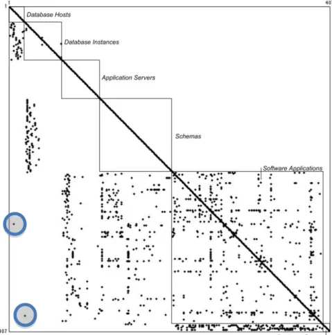
A layered DSM showing the BioPharma enterprise architecture is presented in Figure 1. The matrix is binary with marks in the off-diagonal cells indicating a direct dependency from row to column (and hence a change vulnerability from column to row). White space indicates there is no direct dependency between elements. To set the order of layers we use knowledge of the logical relationships between components. Usage flows from business groups (at the bottom) to applications, from applications to schemas and application servers, from schemas to database instances and from database instances to database hosts (at the top). Within layers, we order components using the component ID, an arbitrary numbering scheme. Note that “communicates with,” the dependency captured between software applications in our data, is bi-directional, hence the marks in the rows and columns of this layer are symmetric around the main diagonal.
§
83
Figure 1. A DSM displaying BioPharma’s layered Enterprise Architecture
Summing the row entries for a given component in the DSM measures the direct outgoing coupling of that component – the number of other components that it uses. We call this measure the direct “fan-out” dependency of the component. Summing the column entries measures the direct incoming coupling of that component – the number of other components that use it. We call this measure the direct “fan-in” dependency of the component. White space to the right of a given layer indicates that components in the layer do not depend on layers below. White space to the left indicates that components in the layer do not depend on layers above.
On the whole, the DSM confirms that this enterprise architecture displays a good separation of concerns: for the most part, schemas act as an interface between applications and the database instances and hosts. Schemas are also efficiently managed: one schema may serve several applications and one application may make use of several schemas. There are two exceptions, however, as indicated by the two circles, where specific applications appear to directly use a database instance or a database host. These exceptions may indicate poor encapsulation or non-standard practices, and hence would be worth investigating further.
84 We note that the Application Interaction Matrix (AIM) is the largest submatrix in this DSM. It shows the dependencies caused by interactions between the software applications in the enterprise’s portfolio. In this dataset, dependencies between software applications are captured by the term “communicates with,” which does not possess directionality (i.e. we do not know which application is requesting a computation and which is performing it). Hence the AIM is symmetric. In general however, capturing information about directionality is always desirable. In particular, one application may always ask for a computation, and another may always supply the result. This distinction would be obscured if all dependencies were merely assumed to be symmetric. However, if applications switch roles, sometimes requesting and sometimes supplying computational services, a symmetric dependency would in fact be warranted.
4
Analyzing an Enterprise Architecture DSM
Figure 1 displays the layered structure of the enterprise architecture, but does not reveal other important architectural characteristics such as indirect coupling, cyclic coupling, hierarchy, or the presence of “core” and “peripheral” components. Matrix operations can be applied to a DSM to analyze these additional features. Specifically, the transitive closure of the matrix reveals indirect dependencies among components in addition to the direct dependencies [20], [83]. That is, if C depends on B and B depends on A, transitive closure reveals that C depends on A.
Applying the procedure of transitive closure to a DSM results in what is called the “Visibility” matrix [20], [75]. The visibility matrix captures all of the direct and indirect dependencies between elements. In a similar fashion to the DSM, row sums of the Visibility matrix, called “visibility fan-out” (VFO) measure the direct and indirect outgoing dependencies for a component. Column sums, called “visibility fan-in” (VFI) measure the direct and indirect incoming dependencies for a component. In a layered enterprise architecture, like the one observed in BioPharma, components at the top of the DSM will have high VFI and components at the bottom of the DSM will have high VFO. Critically, in cases where the systems layers are not known a priori, the Visibility matrix can be sorted using VFI and VFO to reveal the hierarchical relationships among components/layers.**
VFI and VFO can be used to identify “cyclic groups” of components, each of which is directly or indirectly connected to all others in the group. Mathematically, members of the same cyclic group all have the same VFI and VFO measures, given they are all connected directly or indirectly to each other. Thus we can identify cyclic groups in a system by sorting on these measures after performing a transitive closure on the DSM [75]. Large cyclic groups are problematic for system designers, given changes to a component may propagate via a chain of dependencies to many other components. In such a structure, the presence of cyclicality means that there is no guarantee that the design process (or a design change) will converge on a globally acceptable solution that satisfies all components [19], [60].
The density of the Visibility matrix, called Propagation Cost, provides a measure of the level of coupling for the system as a whole. Intuitively, the greater the density of the Visibility matrix, the more ways there are for changes to propagate, and thus the higher the cost of change. Large differences in propagation cost are observed across systems of similar size and function [77]. Yet empirical evidence also suggests that refactoring efforts aimed at making a design more modular can lower propagation cost substantially [20], [85]. These findings suggest that at least for software, architecture is not dictated solely by system function, but varies widely, at the discretion of a system’s architects.
Prior work has shown that the components in a system can be classified into different groups according to the levels of coupling they exhibit, as captured by VFI and VFO. Specifically, Baldwin et al. [75] use DSMs to analyze the structure of 1286 releases from 17 distinct software
**
85 applications. They find the majority of systems exhibit a “core-periphery” structure, characterized by a single dominant cyclic group of components (the “Core”) that is large relative to the system as a whole as well as to other cyclic groups. They show that the components in such systems can be divided into four groups – Core, Peripheral, Shared and Control – that share similar properties in terms of coupling. In such systems, dependencies (i.e. “usage”) flow from Control components, through Core components, to Shared components. This represents the main “flow of control” in the system. Peripheral components, by contrast, lie outside the main flow of control, given they are weakly connected to other system components.
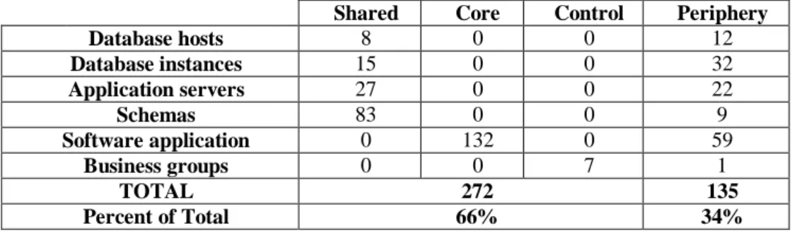
We constructed the Visibility Matrix for BioPharma, and applied the classification methodology described in [75] to the resulting data for VFI and VFO (see Table 1). We find that the firm’s enterprise architecture has a core-periphery structure, with 132 “Core” components (i.e. components that are mutually interdependent). Furthermore, all of the Core components in the system are software applications (but note, not all software applications are classified as Core). Each of the layers in the enterprise architecture identified in Figure 1 has some components that are part of the main flow of control, and others in the “Periphery.” In total, 2/3 of the components in the architecture are part of the main flow and 1/3 are peripheral. We believe managers will find this type of classification scheme useful to set priorities, allocate resources, analyze costs, and understand potential differences in resource productivity.
Table 1. Distribution of Components in the Architecture by Layer and Category
Shared Core Control Periphery
Database hosts 8 0 0 12
Database instances 15 0 0 32
Application servers 27 0 0 22
Schemas 83 0 0 9
Software application 0 132 0 59
Business groups 0 0 7 1
TOTAL 272 135
Percent of Total 66% 34%
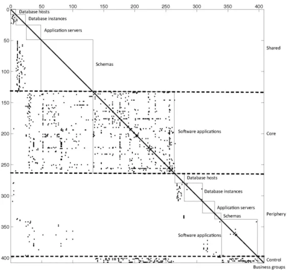
Figure 2 shows a reorganized view of BioPharma’s DSM, organized first, by type of component (i.e. Shared, Core, Periphery, Control) and second, by enterprise architecture layer. We call this the “core-periphery” view of the enterprise architecture DSM. Components in Shared, Core or Control categories are directly or indirectly connected to all Core components (and potentially, other components not in the Core) and hence represent the main flow of control. Thus each main-flow component is connected to at least 132 other components (though the direction of these dependencies will vary by category). In contrast, the highest level of coupling (i.e. visibility fan-in or visibility fan-out) for any peripheral component is only 7. Hence the indirect coupling levels of components in the main flow and the periphery are dramatically different. Assuming the level of component coupling is related to the cost of change, as Parnas [82] suggests, main-flow components will cost significantly more to change than components in the periphery. We investigate this argument empirically in the following section.
5
Using the Enterprise IT Architecture DSM to Predict Performance
86
Figure 2. Reorganized DSM showing Main Flow and Peripheral Components
5.1 The Relationship between Coupling and the Cost of Change
In the previous section, we show that BioPharma’s enterprise architecture is comprised of components with very different levels of coupling. In complex systems, heterogeneous levels of component coupling are the rule, not the exception (e.g. [12], [75], [78], [85]). However, little empirical evidence exists about how different measures of coupling relate to the costs of change for a system’s components. These costs determine the agility of a firm with respect to evolving and adapting its IT systems, hereon called modifiability.
Design theory predicts that the more coupled a component is, the more difficult and expensive it will be to change [59]. However, the components of a system can be connected in different ways. Specifically, they can be connected directly or indirectly; and they can be connected hierarchically or cyclically. Furthermore, components that are hierarchically connected may be at the top or the bottom of the hierarchy, whereas components that are cyclically connected may be members of a large or a small cyclic group. Measures of these (and other) types of coupling can be derived from an enterprise architecture DSM.
In this study, we examine the performance impact of three related coupling measures:
(1)The level of Direct Coupling for each component, which is calculated by summing the entries in the rows and columns of the enterprise architecture DSM.
87
(3)The Closeness Centrality for a component, a metric from social network theory, which can
be calculated for Core components (i.e. those in the same network).††
In our dataset, data on the cost of change was available only for software applications, whose dependency relationships are defined to be symmetric. Hence it was not possible to explore the impact of differences between the number of “incoming” and “outgoing” dependencies, nor differences in the hierarchical classification of components (a symmetric DSM contains Core and Peripheral elements, but no Shared or Control elements). In general however, our method allows the exploration of these issues, in cases where dependencies are asymmetric.
Different measures of coupling are likely to be correlated. Specifically, components with high levels of direct coupling are more likely to be members of the Core. Furthermore, closeness centrality is only defined for components in the Core (i.e. those in the same network). ‡‡ Finally, Core components with high levels of direct coupling are more likely to have higher closeness centrality. Hence we must be sensitive to issues of multi-collinearity. To address this issue, we conduct our analysis in two stages. First, we explore the impact of Direct and Indirect coupling on the cost of change for all applications. Then, for the subset of Core applications, we test whether the measure of closeness centrality provides additional explanatory power.
Stage 1: Direct versus Indirect coupling. Following Chidamber and Kemerer [69], we define direct coupling (DC) as the number of direct dependencies between one software application and all others. Note that because software dependencies are defined as symmetric, the number of incoming and outgoing dependencies is identical. The level of indirect coupling is captured by whether a software application is part of the largest cyclic group (i.e. the Core) in the system. All members of the Core have the same number of direct and indirect dependencies. Core membership is revealed through transitive closure of the DSM.§§
Design theory predicts that higher levels of direct coupling will be associated with higher costs to change. The theory of change propagation predicts that higher levels of indirect coupling (as measured by Core membership) will also lead to higher costs to change. These effects might be additive, or they might be substitutes. We thus state the following hypotheses:
H1: Direct Coupling (DC) is positively associated with change cost (CC).
H2: Core membership (CORE) is positively associated with change cost (CC).
H3: Direct Coupling (DC) and Core membership (CORE), considered together, explain more of the variation in change cost (CC) than either measure considered alone.
We test these hypotheses by performing OLS regressions for the impact of Direct Coupling and Core membership on the cost of change, both individually and together.
Stage 2: Coupling within the Core. For Core components, closeness centrality (CENT) is found by calculating the minimum path length from that component to all other components, summing those path lengths and taking the inverse of this sum [86]. The higher this number, the more “central” is the component. Our final hypothesis explores the possibility that closeness centrality explains variations in change cost for all components that are part of the same cyclic group (i.e. they possess the same high level of indirect coupling):
††
Closeness centrality captures how “close” a component is to other components in a network. But it can only be calculated for symmetric networks. If A depends upon B, but B does not depend upon A, then the path length from A to B, and from B to A will differ. Centrality cannot capture these subtleties. It assumes dependencies are symmetric, which is not the norm in technical systems, but is true for software applications at BioPharma.
‡‡
In prior work, the closeness centrality for elements that have no connections to others is sometimes assumed to be zero (i.e. denoting an infinite path between these and other elements).
§§
88 H4: For components that are members of the Core, closeness centrality (CENT) is positively associated with change cost (CC).
We test this hypothesis by performing an OLS regression for the impact of closeness centrality on the cost of change only for Core components.
5.2 Dependent Variable: The Cost of Change for a Component
To demonstrate our methodology, we use data on the cost of change for software applications. Focusing on a single layer of the firm’s enterprise architecture (i.e. as opposed to all layers) allowed us to i) identify a specific respondent for data collection, ii) request quantitative data from these respondents, and iii) ensure the data was comparable across units.
The cost to change of each application was assessed via a survey sent to IT Service Owners. Respondents were asked to estimate the time, in person-years, to perform five IT operations: deploy, upgrade, replace, decommission, and integrate. Operations were defined as follows: “A component is deployed when it is put into production for the first time; a component is upgraded when it is replaced by a new version of the same component; a component is replaced when the existing component is removed from the information system and a new component with similar functionality is added to the information system; a component is decommissioned when it is removed from the information system; and a component is integrated when modifications are made to it that enable it to 'talk' to another component”.***
We received survey responses for 99 software applications. The change cost estimates ranged from less than one-person-month to over two-person-years. Respondents could also indicate that the time to perform a given operation was unknown. Applications for which all change costs were unknown were removed from the dataset, resulting in a final sample of 77 applications. For these applications, we combined the change cost estimates for different operations into a single measure, by calculating the mean change cost for operations where a response was provided. The Cronbach’s alpha for this aggregate measure was 0.78.†††
5.3 Control Variables
Change costs may be affected by a number of factors that are unrelated to architecture, including the source of the component, the users of the component, its internal structure, and whether it was the focus of active development at the time of the survey. In addition, the respondent’s experience with a given component might affect the appraisal of change cost in a systematic way. Hence data on the following variables were collected and included as controls:
(1)VENDOR indicates whether an application is developed by a vendor (1) or in-house (0). One
component missing data for this variable was assigned a value of 0.5.‡‡‡
(2)CLIENT indicates whether an application is accessed by end-users (1) or not (0).
(3)COMP indicates whether an application is focused on computation (1) or not (0).
(4)NTIER indicates whether an application has an N-tier architecture (1) or some other type of
architecture, such as client-server or monolithic (0).
(5)ACTIVE indicates whether, at the time of the survey, the component was being actively
enhanced (1) or was in maintenance mode (0).
***
Specifically, we asked respondents to estimate whether the effort (in person-years) required for each operation fell into the following ranges: <0.10, 0.10-0.249, 0.25-0.49, 0.50-0.99, 1.00-1.99, and > 2.00. The resulting dependent variable was an integer ranging from 1 to 6.
†††
Where the estimate of change cost for an operation is missing, we substitute the mean level of change cost for that operation from all respondents to calculate Cronbach’s alpha. Other ways of treating missing values result in a minimum value for alpha of 0.66 (acceptable) to a maximum value of 0.89 (extremely good).
‡‡‡
89
(6)RES_EXP measures the respondent’s experience with the application in question (less than
one year = 1; 1–5 years = 2; more than 5 years = 3).
5.4 Empirical Data
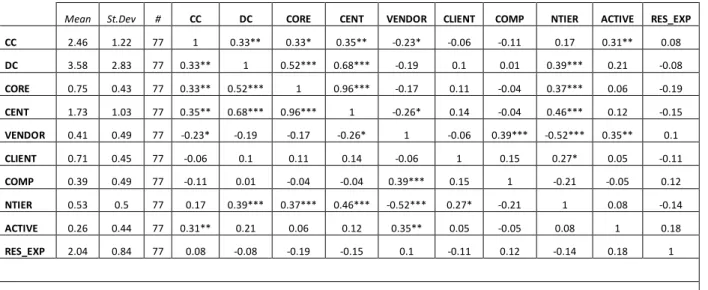
Table 2 presents the correlation matrix for our variables. Consistent with our hypotheses, both direct coupling (DC) and CORE are positively correlated with change cost. They are also correlated with each other (0.52). In this table, we include data on closeness centrality (CENT) for the entire sample of 77 applications, substituting a value of 0 for the 19 components not in the Core. Hence we observe an extremely high correlation (0.96) between CORE and CENT.
Among the control variables, Active components tend to have higher change costs. Vendor provided components tend to have lower change costs, have lower centrality, are more likely to perform computations, are less likely to have N-tier architectures, and are more likely to be Active. Components with N-tier architectures tend to be more highly coupled by all measures.
Table 2. Descriptive Statistics and Correlation Matrix
Mean St.Dev # CC DC CORE CENT VENDOR CLIENT COMP NTIER ACTIVE RES_EXP
CC 2.46 1.22 77 1 0.33** 0.33* 0.35** -0.23* -0.06 -0.11 0.17 0.31** 0.08
DC 3.58 2.83 77 0.33** 1 0.52*** 0.68*** -0.19 0.1 0.01 0.39*** 0.21 -0.08
CORE 0.75 0.43 77 0.33** 0.52*** 1 0.96*** -0.17 0.11 -0.04 0.37*** 0.06 -0.19
CENT 1.73 1.03 77 0.35** 0.68*** 0.96*** 1 -0.26* 0.14 -0.04 0.46*** 0.12 -0.15
VENDOR 0.41 0.49 77 -0.23* -0.19 -0.17 -0.26* 1 -0.06 0.39*** -0.52*** 0.35** 0.1
CLIENT 0.71 0.45 77 -0.06 0.1 0.11 0.14 -0.06 1 0.15 0.27* 0.05 -0.11
COMP 0.39 0.49 77 -0.11 0.01 -0.04 -0.04 0.39*** 0.15 1 -0.21 -0.05 0.12
NTIER 0.53 0.5 77 0.17 0.39*** 0.37*** 0.46*** -0.52*** 0.27* -0.21 1 0.08 -0.14
ACTIVE 0.26 0.44 77 0.31** 0.21 0.06 0.12 0.35** 0.05 -0.05 0.08 1 0.18
RES_EXP 2.04 0.84 77 0.08 -0.08 -0.19 -0.15 0.1 -0.11 0.12 -0.14 0.18 1
* p<0.05, ** p<0.01, and ***p<0.001
5.5 Empirical Results
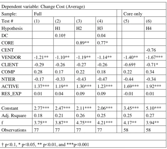
The results of our regression tests are presented in Table 3. Model 1 contains only controls, showing that two of them are significant: Vendor provided applications tend to have lower change costs and Active applications tend to have higher change costs. The control variables alone explain 18% of the variation in change cost across applications.
Our first hypothesis, H1 predicts that direct coupling is associated with change cost, a relationship suggested by the correlations reported above. In Model 2 however, which includes control variables, we find direct coupling is only a relatively weak predictor of change cost (p-value = 0.06). This model explains 21% of the variation in change cost across applications. In Model 3, we find CORE is a highly significant predictor of change cost (p-value = 0.005). This model explains 26% of the variation in change cost across components, supporting H2.
90
Table 3. Regression Models
Dependent variable: Change Cost (Average)
Sample: Full Core only
Test # (1) (2) (3) (4) (5) (6)
Hypothesis H1 H2 H3 H4
DC 0.10† 0.04
CORE 0.89** 0.77*
CENT -0.76
VENDOR -1.21** -1.10** -1.19** -1.14** -1.40** -1.67*** CLIENT -0.29 -0.26 -0.27 -0.26 -0.69† -0.71*
COMP 0.28 0.17 0.22 0.18 0.22 0.34
NTIER -0.17 -0.33 -0.43 -0.47 -0.44 -0.34 ACTIVE 1.37*** 1.19** 1.30*** 1.23*** 1.69*** 1.92*** RES_EXP 0.01 0.04 0.09 0.09 -0.01 0.01
Constant 2.77*** 2.47*** 2.11*** 2.06*** 3.45*** 5.10*** Adj. Rsquare 0.18 0.21 0.26 0.25 0.25 0.27 f 3.75** 3.87** 4.75*** 4.21*** 4.17** 3.94**
Observations 77 77 77 77 58 58
† p<0.1, * p<0.05, ** p<0.01, and ***p<0.001
In models 5 and 6, we analyze only the 59 components in the Core (the largest cyclic group of components). Model 5 contains only control variables, and produces results consistent with Model 1. Model 6 includes the measure of closeness centrality, which is not significant. Hence closeness centrality provides no additional explanatory power in predicting change cost, over and above that provided by Core. We therefore reject hypothesis H4.
5.6 Robustness Checks
We performed a number of checks to assess whether our results were sensitive to other assumptions or specifications of variables. First, we note that our basic specification did not control for the size of components, a variable that could plausibly affect the cost of changes. Data on component size (measured by the number of lines of code and files in each) was available for a subsample of 60 applications. We ran our models on this smaller sample, including these as controls. The controls were insignificant, while the results for our explanatory variables were consistent with those reported above.§§§
We conducted a test to explore the possibility that transformations of direct coupling might better predict change cost, given this variable has a skewed distribution and is truncated at zero. Specifically, we included the natural log of direct coupling in models, instead of the raw value. We found the transformed variable had more explanatory power than the raw variable (i.e. its use improved the results in Model 2). However, it still explained less of the variation in change cost than CORE, hence was insignificant when included in a model with CORE.
Finally, we explored whether direct coupling, or its natural log, contribute to explaining the variation in change cost among only Core components (as we did for centrality). Appendix reports the results of three models predicting change cost, the first being a model with controls, the second adding direct coupling, and the third adding the natural log of direct coupling. Direct
§§§
91 coupling is not statistically significant in any model. This suggests that in this dataset, CORE is the most parsimonious and powerful measure of coupling that explains the cost of change. Neither direct coupling, nor centrality, contributes additional explanatory power in our models.
6
Discussion and Conclusions
The main contribution of this article is in developing a robust and repeatable network-based methodology by which to operationalize a firm’s enterprise IT architecture. The methodology is consistent with prior work in this area, and addresses several limitations of this work. Specifically, it i) integrates the consideration of business and IT related attributes; ii) identifies distinct layers in the architecture associated with different entities (e.g. applications, databases, etc.); iii) reveals the “flow of control” within the architecture across its associated layers and; iv) generates measures of the architecture that can be used to predict performance. We demonstrate the application of this methodology to predict IT modifiability using a real-world dataset, and show that it generates insights that could not have been gained merely from the inspection of documents or processes traditionally associated with EA frameworks.
A second contribution of this article lies in the specific results we report using our methodology to analyze enterprise architecture. Specifically, we explore the relationship between measures of coupling derived from a DSM, and IT modifiability – defined as the cost of change for software applications. The measure of coupling that best predicts change cost is not the number of direct dependencies for a component, but all of the direct and indirect dependencies it has with other components. Once the variation in change cost explained by this measure is accounted for, other measures of coupling add no further explanatory power. This suggests a firm’s agility to adapt its IT infrastructure (modifiability) is driven mainly by the potential for changes to propagate from one component to others via chains of dependencies. Such data is not visible from inspection of a component’s “nearest neighbors.” Rather, our findings lend support to the methods we employ, which reveal all of the indirect paths that exist between system components.
For managers, our methodology provides a clear picture of the actual instantiated architecture that they possess, as opposed to high level conceptual representations often found in documents depicting a firm’s IT architecture. The insights thereby generated will prove useful in several ways, including i) helping to plan the allocation of resources to different components, based upon predictions of the relative ease/difficulty of change; ii) monitoring the evolution of an architecture over time, as new components and/or dependencies are introduced (e.g. when a new firm is acquired) and; iii) identifying opportunities to improve the architecture, for instance, by reducing coupling, and hence reducing the cost to change specific components.
92 important dependencies between components in a firm’s enterprise architecture. ****
This implies the need for some investment by firms who wish to adopt these methods. We believe the benefits associated with these investments would more than offset the costs, given the increase in understanding of the firm’s IT architecture that would result.
For the academy, this study contributes to the field of enterprise IT architecture in several ways. First, it makes what has been a rather conceptual area more grounded, providing a method to analyze a firm’s architecture in-use, rather than the processes and documents through which it is created and managed. Second, it provides a way to operationalize frameworks like TOGAF [1], defining how the matrices they include can be quantified and analyzed. Finally, our methodology generates metrics that capture the level of coupling between different components in a firm’s IT architecture, reveals the main “flow of control” across the system, and allows us to examine how IT modifiability might vary for different system components.
Our work opens up the potential for further empirical research that could explore the relationship between enterprise architecture and performance. Within organizations, work might focus on the relationship between measures of coupling, and a variety of performance measures relevant to individual components in the architecture (e.g. reliability, security, productivity). In contrast, studies across different organizations might reveal how measures of enterprise architecture affect firm-level performance. The latter area is particularly promising, given prior literature argues there is a strong linkage between certain types of architecture and firm-level attributes, such as agility. One might ask, for instance, whether loosely coupled architectures, in general, facilitate a rapid response to unpredictable business challenges? Or are there subtle nuances to account for, with respect to different layers in the architecture (e.g. is the use of shared databases – with the pattern of coupling this entails – a best practice)? This methodology allows us to answer such questions, with an approach that can be replicated across studies.
Our study is subject to a number of limitations that must be considered when assessing the generalizability of results. In particular, the data to demonstrate our methods comes from a single firm. Hence more work is needed to provide validation of these methods across different contexts. Furthermore, questions remain as to the different layers/components that should be included in the analysis of enterprise IT architecture, and the types of dependency that exist between them. For instance, we may find that different types of dependency (e.g. “uses” versus “communicates with”) predict different dimensions of performance (e.g. modifiability versus reliability). Similarly, we may find that different measures of coupling (e.g. direct versus indirect coupling) may predict performance differently across different contexts. Ultimately, our methods provide a platform to enable researchers to answer a variety of questions that until now have proved elusive. As such, we hope that future scholars will improve upon and evolve these methods, in order that we benefit from the cumulative nature of enterprise IT knowledge.
References
[1] The Open Group, “The Open Group Architecture Framework(TOGAF),” Version 9.2, 2018.
[2] R. Foorthuis, M. Van Steenbergen, S. Brinkkemper, and W. A. Bruls, “A theory building study of enterprise architecture practices and benefits,” Information Systems Frontiers, vol. 18, no. 3, pp. 541–564, 2016. Available: https://doi.org/10.1007/s10796-014-9542-1
[3] M. Lange, J. Mendling, and J. Recker, “An empirical analysis of the factors and measures of Enterprise Architecture Management success,” European Journal of Information Systems, vol. 25, no. 5, pp. 411–431, 2016. Available: https://doi.org/10.1057/ejis.2014.39
[4] J. Lapalme, A. Gerber, A. Van der Merwe, J. Zachman, M. De Vries, and K. Hinkelmann, “Exploring the future of enterprise architecture: A Zachman perspective,” Computers in Industry, vol. 79, pp. 103–113, 2016. Available: https://doi.org/10.1016/j.compind.2015.06.010
****
93
[5] M. van den Berg, R. Slot, M. van Steenbergen, P. Faasse, and H. van Vliet, “How enterprise architecture improves the quality of IT investment decisions,” Journal of Systems and Software, vol. 152, pp 134–150, 2019. Available: https://doi.org/10.1016/j.jss.2019.02.053
[6] L. Halawi, R. McCarthy, and J. Farah, “Where We are with Enterprise Architecture,” in Proceedings of the Conference on Information Systems Applied Research, vol. 2167, p. 1508, 2018.
[7] G. Shanks, M. Gloet, I. A. Someh, K. Frampton, and T. Tamm, “Achieving benefits with enterprise architecture,” The Journal of Strategic Information Systems, vol. 27, no. 2, pp. 139–156, 2018. Available: https://doi.org/10.1016/j.jsis.2018.03.001
[8] Y. Gong, and M. Janssen, “The value of and myths about enterprise architecture,” International Journal of Information Management, vol. 46, pp. 1–9, 2019. Available: https://doi.org/10.1016/j.ijinfomgt.2018.11.006 [9] E. T. Vakkuri, “Developing Enterprise Architecture with the Design Structure Matrix,” Master Thesis.
Tampere University of Technology, Finland, 2013.
[10]R. O. Stroud, A. Ertas, and S. Mengel, “Application of Cyclomatic Complexity in Enterprise Architecture Frameworks,” IEEE Systems Journal, 2019. Available: https://doi.org/10.1109/JSYST.2019.2897592
[11]A. Santana, A. Souza, D. Simon, K. Fischbach, and H. De Moura, “Network Science Applied to Enterprise Architecture Analysis: Towards the Foundational Concepts,” IEEE 21st International Enterprise Distributed Object Computing Conference (EDOC), pp. 10–19, IEEE, October 2017. Available: https://doi.org/10.1109/EDOC.2017.12
[12]R. Lagerström, C. Baldwin, A. MacCormack, and D. Dreyfus, “Visualizing and measuring enterprise architecture: an exploratory biopharma case,” IFIP Working Conference on The Practice of Enterprise Modeling, pp. 9–23, 2013. Available: https://doi.org/10.1007/978-3-642-41641-5_2
[13]P. Weill, “Innovating with Information Systems: What do the most agile firms in the world do,” Proceedings of the 6th e-Business Conference, Barcelona, 2007.
[14]Tanredi, H. A. Rai, and N. Venkatraman. “Reframing the dominant quests of information systems strategy research for complex adaptive business systems,” Information Systems Research, vol. 21, no. 4, 2010. Available: https://doi.org/10.1287/isre.1100.0317
[15]A. Tiwana, B. Konsynski, and A. Bush. “Platform Evolution: Coevolution of platform architecture, governance and environmental dynamics,” Information Systems Research, vol. 21, no. 4, 2010. Available: https://doi.org/10.1287/isre.1100.0323
[16]F. Gampfer, “Managing Complexity of Digital Transformation with Enterprise Architecture,” 31st Bled E-conference Digital Transformation: Meeting The Challenges, pp. 635–642, 2018. Available: https://doi.org/10.18690/978-961-286-170-4.44
[17]A. Tiwana, and B. Konsynski, “Complementarities between organizational IT architecture and governance structure,” Information Systems Research, vol. 21, no. 2, 2010. Available: https://doi.org/10.1287/isre.1080.0206
[18]P. Johnson, R. Lagerström, M. Ekstedt, and M. Österlind, “IT Management with Enterprise Architecture,” ePub, KTH Royal Institute of Technology, Stockholm, 2014.
[19]D. Steward, “The design structure system: A method for managing the design of complex systems,” IEEE Transactions on Engineering Management, vol. EM-28, no. 3, pp. 71–74, 1981. Available: https://doi.org/10.1109/TEM.1981.6448589
[20]A. MacCormack, J. Rusnak, and C. Baldwin, “Exploring the structure of complex software designs: an empirical study of open source and proprietary code,” Management Science, vol. 52, no. 7, pp. 1015–1030, 2006. Available: https://doi.org/10.1287/mnsc.1060.0552
[21]O. Bjuhr, K. Segeljakt, M. Addibpour, F. Heiser and R. Lagerström, “Software architecture decoupling at Ericsson,” in Proceedings of the IEEE International Conference on Software Architecture (ICSA), 2017. Available: https://doi.org/10.1109/ICSAW.2017.7
[22]S. Aier, and R. Winter, “Virtual decoupling for IT/business alignment–conceptual foundations, architecture design and implementation example,” Business & Information Systems Engineering, vol. 1, no. 2, pp. 150–163, 2009. Available: https://doi.org/10.1007/s12599-008-0010-7
[23]ISO/IEC/IEEE, Systems and software engineering – Architecture description. Technical standard, 2011. [24]M. Rohloff, “Framework and Reference for Architecture Design,” Proceedings of the Americas' Conference on