ORIGINAL RESEARCH ARTICLE
Optimal DG placement for benefit
maximization in distribution networks by using
Dragonfly algorithm
M. C. V. Suresh
1*and Edward J. Belwin
2Abstract
Distributed generation (DG) is small generating plants which are connected to consumers in distribution systems to improve the voltage profile, voltage regulation, stability, reduction in power losses and economic benefits. The above benefits can be achieved by optimal placement of DGs. A novel nature-inspired algorithm called Dragonfly algorithm is used to determine the optimal DG units size in this paper. It has been developed based on the peculiar behavior of dragonflies in nature. This algorithm mainly focused on the dragonflies how they look for food or away from enemies. The proposed algorithm is tested on IEEE 15, 33 and 69 test systems. The results obtained by the proposed algorithm are compared with other evolutionary algorithms. When compared with other algorithms the Dragonfly algorithm gives best results. Best results are obtained from type III DG unit operating at 0.9 pf.
Keywords: Dragonfly algorithm, Loss sensitivity factor method, Distributed generation placement, Radial distribution system, Loss reduction
© The Author(s) 2018. This article is distributed under the terms of the Creative Commons Attribution 4.0 International License (http://creat iveco mmons .org/licen ses/by/4.0/), which permits unrestricted use, distribution, and reproduction in any medium, provided you give appropriate credit to the original author(s) and the source, provide a link to the Creative Commons license, and indicate if changes were made.
Introduction
Interconnection of generating, transmitting and distribu-tion systems usually called as electric power system. Usu-ally distribution systems are radial in nature and power flow is unidirectional. Due to ever growing demand modern distribution networks are facing several prob-lems. With the installation of different distributed power sources like distributed generations, capacitor banks etc, several techniques have been proposed in the literature for the placement of DGs. Most of the losses about 70% losses are occurring at distribution level which includes primary and secondary distribution system, while 30% losses occurred in transmission level. Therefore, distribu-tion systems are main concern nowadays. The losses tar-geted at distribution level are about 7.5%.
By installing DG units at appropriate positions, the losses can be minimized. Photovoltaic (PV) energy, wind turbines, and other distributed generation plants are
typically situated in remote areas, requiring the opera-tion systems that are fully integrated into transmission and distribution network. The aim of the DG is to inte-grate all generation plants to reduce the loss, cost and greenhouse gas emission. The main reason for using DG units in power system is technical and economic benefits that have been presented as follows. Some of the major advantages are (Reddy et al. 2016, 2017c)
• Reduced system losses
• Voltage profile improvement
• Frequency improvement
• Reduced emissions of pollutants
• Increased overall energy efficiency
• Enhanced system reliability and security
• Improved power quality
• Relieved Transmission & Distribution congestion
Some of the major economic benefits
• Deferred investments for upgrades of facilities
• Reduced fuel costs due to increased overall efficiency
Open Access
*Correspondence: [email protected]
1 Department of EEE, S V College of Engineering, Tirupati, Andhra Pradesh, India
• Reduced reserve requirements and the associated
costs
• Increased security for critical loads.
Different types of distributed generations and their defi-nitions have been discussed in Ackermann et al. (2001). An analytical approach was proposed by Acharya et al. (2006) and Hung et al. (2010) with out taking voltage constraint. The uncertainties in operation including varying load, network configuration and voltage control devices have been considered in Su (2010). Sensitivity-based simultaneous optimal placement of capacitors and DG was proposed in Naik et al. (2013). In this paper ana-lytical approach is used for sizing.
Abu-Mouti and El-Hawary (2010) proposed ABC to find the optimal allocation and sizing of distributed gen-eration. Distributed generation uncertainties (Zangiabadi et al. 2011) have been taken in account for the placement of DG.
Alonso et al. (2012), Rahim et al. (2012), Doagou-Mojarrad et al. (2013) and Hosseini et al. (2013) proposed evolutionary algorithms for the placement of distributed generation. Nekooei et al. (2013) proposed Harmony Search algorithm with multi-objective placement of DGs.
A novel combined hybrid method GA/PSO is pre-sented in Moradi and Abedini (2011) for DG placement. With unappropriated DG placement, can increase the system losses with lower voltage profile. The proper size of DG gives the positive benefits in the distribution sys-tems. Voltage profile improvement, loss reduction, dis-tribution capacity increase and reliability improvements are some of the benefits of system with DG placement (Rahim et al. 2013; Ameli et al. 2014).
Embedded Meta Evolutionary-Firefly Algorithm (EMEFA) was proposed in Rahim et al. (2013) for DG allocation. Here how losses are varied with popula-tion size are considered. Simultaneous placement of DGs and capacitors with reconfiguration was proposed by Esmaeilian and Fadaeinedjad (2015) and Golshan-navaz (2014). Dynamic load conditions have been taken in Gampa and Das (2015). Big bang big crunch method was implemented for the placement of DG in Hegazy et al. (2014). Murty and Kumar (2014) uses mesh distri-bution system analysis for the placement of distributed generation with time varying load model. Probabilistic approach with DG penetration was discussed in Kolenc et al. (2015). The backtracking search optimization algo-rithm (BSOA) was used in DS planning with multi-type DGs in El-Fergany (2015), BSOA was proposed for DG placement with various load models.
Reddy et al. (2017a) and Reddy et al. (2017b) proposed whale optimization and Ant Lion optimization algorithm
for sizing of DGs. In most of the studies economic analy-sis has not been taken.
A novel nature-inspired algorithm called Dragon-fly algorithm is used to find the optimal DG size in this paper. The optimal size of DGs at different power factors are determined by DA algorithm to reduce the power losses in the distribution system as much as possible and enhancing the voltage profile of the system. The eco-nomic analysis of DG placement is also considered in this paper.
Problem formulation Objective function
In distribution system more losses are there due to low voltage compared to transmission system. Copper losses predominant in distribution system, this can be calcu-lated as follows
where Ii is current, Ri is resistance and n is number of
buses. Objective taken in this paper is real power loss minimization.
Constraints The constraints are
• Voltage constraints
• Power balance constraints
• Upper and lower limits of DG
where the limits are in kW, kVAr and kVA for Type I, II and III DG, respectively.
Loss sensitivity factors method
Optimal locations for DG placement are identified based on the losses at the nodes and their sensitivity after com-pensation using the loss sensitivity factors method. Real and reactive power losses are calculated at all the buses and then the locations corresponding to the bus which has the highest loss is selected as the best location for DG placement. The buses with high losses give maxi-mum loss reduction when DG are placed in the distribu-tion system. Loss sensitivity is referred to as the change
(1) Ploss=
n
i Ii2Ri
(2) 0.95≤Vi ≤1.05
(3) P+
N
k=1
PDG =Pd+Ploss
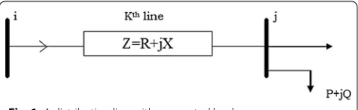
in losses corresponding to the compensation provided by placing the DGs. Loss sensitivity factors (LSF) deter-mine the best locations for DG placement. These factors reduce the search space by finding the few best locations which saves the cost of the DGs in optimizing the losses in the system as a whole. Consider a line with impedance (R + jX) between buses i and j and a load in the distribu-tion system as shown in Fig. 1.
Real power loss in the kth line considered in Fig. 1 is given by [Ik2] × [Rk] and can also be expressed as follows
Similarly reactive power loss in the kth line is given by
[Ik2] × [Xk] and can also be expressed as follows
where Ik is the current flowing through kth line; Rk and
Xk are the resistance and reactance of the kth line; V[j]
is the voltage at the bus j; P[j] = Net Active power sup-plied beyond the bus j; Q[j] = Net Reactive power sup-plied beyond the bus j.
After finding the real and reactive power losses for all the buses, the loss sensitivity factors can be calculated using the following equations.
Identification of optimal locations using loss sensitivity factors
The loss sensitivity factors for all the buses from load flows are calculated using Eq. (7) and the buses are stored in a vector according to their positions such that these factors are arranged in the decreasing order. Voltage magnitudes are normalized by assuming the minimum voltage value as 0.95 at these buses using the following equation
where V[i] is the base voltage at the ith bus. The opti-mal locations for DG placement are determined based on the normalized voltage magnitudes and the loss sen-sitivity factors calculated as described above, the former decides the requirement of compensation and the latter gives the order of priority. The buses with Vnorm≤1.01 are selected as the best suitable locations for the place-ment of DGs in order to reduce the real power losses and improve the voltage profile simultaneously so that the
(5) PL(j)= (P
2(j)+Q2(j))×R k V(j)2
(6) QL(j)= (P
2(j)+Q2(j))×X
k V(j)2
(7) ∂PL
∂Q =
(2×Q(j))×Rk
V(j)2
(8) ∂QL
∂Q =
(2×Q(j))×Xk V(j)2
(9) Vnorm[i] = |V(i)|
0.95
power delivering capacity is enhanced. The value 1.01 is selected as the maximum value of the normalized voltage at the buses where compensation is required.
Algorithm
The algorithm to find the optimal locations for DG place-ment using LSF is explained in detail in the following steps
Step 1 Read line and load data of the system and solve the feeder line flow for the system using the branch current load flow method.
Step 2 Calculate the real and reactive power losses using Eqs. (5) and (6).
Step 3 Find the loss sensitivity factors using Eq. (7). Step 4 Store the buses with loss sensitivity
fac-tors arranged in decreasing order in a vector according to their positions.
Step 5 Normalize the magnitudes of the voltages for all the buses using Eq. (9).
Step 6 Select the buses with normalized voltage mag-nitudes less than 1.01 as the best suitable loca-tions for DG placement.
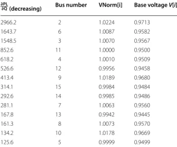
LSF method is applied to 15-bus, 33-bus and 69-bus IEEE systems and the locations are given in the tables below (Tables 1, 2, 3).
15-bus system
From above table first best location for DG placement is 6.
33-bus system
From above table first best location for DG placement is 6.
69-bus system
From above table first best location for DG placement is 61.
The Dragonfly algorithm (DA)
The DA algorithm was proposed by Mirjalili (2015). It has been developed based on swarm intelligence and the peculiar behavior of dragonflies in nature. This algorithm mainly focused on the dragonflies how they look for food or away from enemies.
The static behavior of dragonflies, i.e, looking for food can be treated as exploitation phase and evade from enemies can be treated as exploration phase. The static swarm dragonflies consist of small group of dragonflies which are hunting the preys in small space. The direc-tion and velocity of this dragonflies are small and abrupt changes will be there in the direction. Dynamic swarm with constant direction and more number of different dragonflies moves to another place over a long distance.
The mathematical model of DA algorithm can be mod-eled with the following five behaviors of dragonflies.
Separation In the static swarm no collision is there between any dragonflies. The mathematical model Si of
the ith individual is given by
Here
Position of current dragonflies is represented by X
Xk represents position of kthneighboring dragonflies N is the total number of neighboring dragonflies
Alignment Individual dragonflies velocities will match with the other in same neighborhood. This can be mod-eled as
where Vk is the velocity of the kth neighboring individuals
Cohesion All the dragonflies will move toward the cen-tre of mass of the neighborhood. This can be modeled as
Food For survival all the dragonflies will move toward the food. The attraction for food can be modeled as
where XF is the position of food location.
Enemy All the dragonflies will move away from an enemy. To move away from the enemy located at a posi-tion XE can be modeled as
All the above five motions will influence the behavior of dragonflies in the swarm. The new position update of dragonflies can be obtained with the following step func-tion ∆Xi+1 which is modeled as
where separation, alignment, cohesion weights, food, enemy factors and inertia factor are represented by s, a, c, f, e and w, respectively
With the above step function the new position of Xi+1 is given by
The best and worst solutions are taken from food source and enemy. If there is no neighboring solution, DA can be (10) Si = −
N
k=1
X−Xk
(11) Ai=
N k=1Vk
N
(12) Ci=
N k=1Xk
N −X
(13) Fi=XF−X
(14) Ei=XE+X
(15) ∆Xi+1=(sSi+aAi+cCi+f Fi+eEi)+w∆Xi
(16) Xi+1=Xi+∆Xi+1
Table 1 Loss sensitivity factors for 15-bus system
∂PL
∂Q (decreasing) Bus number VNorm[i] Base voltage V[i]
2966.2 2 1.0224 0.9713
1643.7 6 1.0087 0.9582
1548.5 3 1.0070 0.9567
852.6 11 1.0000 0.9500
618.2 4 1.0010 0.9509
526.6 12 0.9956 0.9458
413.4 9 1.0189 0.9680
314.1 15 0.9984 0.9484
292.6 14 0.9985 0.9486
281.1 7 1.0063 0.9560
167.8 13 0.9942 0.9445
161.3 8 1.0073 0.9570
134.2 10 1.0178 0.9669
125.6 5 0.9999 0.9499
Table 2 Loss sensitivity factors for 33-bus system
∂PL
∂Q (decreasing) Bus number VNorm[i] Base voltage V[i]
1678 6 0.9995 0.9495
1365 28 0.9827 0.9335
1325 3 1.035 0.9829
Table 3 Loss sensitivity factors for 69-bus system
∂PL
∂Q (decreasing) Bus number VNorm[i] Base voltage V[i]
2664.8 57 0.9896 0.9401 1344.9 58 0.9779 0.9290
935.7 7 1.0324 0.9808
882.9 6 1.0422 0.9901
848.3 61 0.9604 0.9123
635.0 60 0.9681 0.9197
571.8 10 1.0236 0.9724
526.9 59 0.9734 0.9248
456.8 55 1.0178 0.9669
modeled through random walk. New position of dragon-flies is updated with following equations.
where random numbers r1,r2 ε [0,1] , i is current iteration, d is dimension and β is equal to 1.5.
Implementation of DA
The detailed algorithm is as follows.
Step 1 Feeder line flow is solved by branch current load flow method.
Step 2 Find the best DG locations using the index vector method.
Step 3 Initialize the population/solutions and itmax = 100, Number of DG locations d=1,dgmin=60,dgmax=3500.
Step 4 Generate the population of DG sizes ran-domly using equation
population=(dgmax−dgmin)×rand()+dgmin where dgmin and dgmax are minimum and max-imum limits of DG sizes.
Step 5 Determine active power loss for generated population by performing load flow.
Step 6 Select low loss DG as current best solution. Step 7 Update the position of the dragonflies using
Eqs. 11–13.
Step 8 Determine the losses for updated population by performing load flow.
Step 9 Replace the current best solution with the updated values if obtained losses are less than the current best solution. Otherwise go back to step 7
Step 10 If maximum number of iterations is reached then print the results.
Results and discussion
DA algorithm in the application of DG planning problem to obtain DG size and economic analysis is presented in this section. IEEE 15, 33 and 69 bus test systems are eval-uated using MATLAB.
Economic analysis
The mathematical model is given below for cost calculations.
(17) Xi+1=Xi+Levy(x)×Xi
Levy(x)=0.01×r1×σ |r2|
1
β
σ =
Ŵ(1+β)×sin��β2 �
Ŵ�1+β2 �×β×2
�β−1 2
�
1
β
Ŵ(x)=(x−1)!
Cost of energy losses (CL)
The annual cost of energy loss is given by (Murthy and Kumar 2013)
where TRPL, total real power losses; Kp, annual demand cost of power loss ($/kW); Ke, annual cost of energy loss($/kW h); Lsf, loss factor
Loss factor is expressed in terms of load factor (Lf) as below
The values taken for the coefficients in the loss factor cal-culation are: k = 0.2, Lf = 0.47, Kp = 57.6923 $/kW, Ke = 0.00961538 $/kWh.
Cost component of DG for real and reactive power
Cost coefficients are taken as:
Cost of reactive power supplied by DG is calculated based on maximum complex power supplied by DG as
Pgmax = 1.1*pg, the power factor, has been taken 1 at unity power factor and 0.9(lag) at lagging power factor to carry out the analysis. k=0.05−0.1 . In this paper, the
value of factor k is taken as 0.1.
IEEE 15‑bus system
The single-line diagram of IEEE 15-bus distribution sys-tem (Baran and Wu 1989) is shown in Fig. 2.
Table 4 shows the real,reactive power losses and mini-mum voltages after the placement of different types of DGs. The optimal location for 15 bus test system is 6. The minimum voltage is more in case of type III DG operat-ing at 0.9 pf. The losses are also lower with DG type III operating at 0.9 pf when compared to DG operating at upf in Table 4. This is due to both real and reactive pow-ers are supplied by the DG at lagging pf. Reactive power is not supplied by type III DG when operating at Unity pf. Hence, losses are higher when compared to DG operat-ing at 0.9 pf laggoperat-ing.
Cost of energy losses, cost of PDG and cost of QDG are also shown in Table 4. From table the cost of energy (18) CL=(TRPL)∗(Kp+Ke∗Lsf ∗8760) $
(19) Lsf =k∗Lf +(1−k)∗Lf2
(20) C(Pdg)=a∗Pdg2+b∗Pdg+c $/MWh
a=0, b=20, c=0.25
(21)
C(Qdg)=
Cost(Sgmax)−Cost
Sgmax2−Qg2
∗k
(22) Sgmax= Pgmax
losses is reduced from 4970.3 $ to 2685.3 $ when DG is operating at 0.9pf lag and it reduced to 3684.1 $ when operating at unity pf. Cost of energy losses are less when DG is operating at 0.9pf.
Results for 33 bus
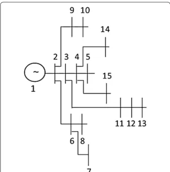
The single-line diagram of IEEE 33-bus distribution sys-tem (Baran and Wu 1989) is shown in Fig. 3.
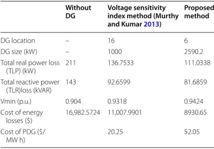
Without installation of DG, real and reactive power losses are 211 kW and 143 kVAr, respectively. With installation of DG at unity pf, real, reactive power losses are 111.0338 kW and 81.6859 kVAr, respectively. With DG at 0.9 pf lag, real, reactive power losses are 70.8652 kW and 56.7703 kVAr, respectively.
The losses obtained are lower when lagging power fac-tor DG is used when compared to unity power facfac-tor DG. This is due to reactive power available in lagging power factor DG.
Cost of energy losses, cost of PDG and cost of QDG are also shown in Tables 5 and 6. From table the cost of energy losses is reduced from 16,982.57 $ to 5700.1 $ when DG is operating at 0.9pf lag and it reduced to 8930.65 $ when operating at unity pf. Cost of energy losses are less when DG is operating at 0.9pf.
Results for 69 bus
The IEEE 69-bus distribution system with 12.66-kV base voltage (Baran and Wu 1989) is shown in Fig. 4.
Without DG real, reactive power losses are 225 kW and 102.1091 kVAr, respectively. With the installation of DG at unity pf, the real and reactive power losses are 83.2261 kW and 40.5754 kVAr, respectively. With DG at 0.9 pf lag real, reactive power losses are 27.9636 kW and 16.4979 kVAr.
The losses obtained are lower when lagging power fac-tor DG is used when compared to unity power facfac-tor DG. This is due to reactive power available in lagging power factor DG.
Cost of energy losses, cost of PDG and cost of QDG are also shown in Tables 5 and 6. From table the cost of energy losses is reduced from 18,101.7 $ to 2249.2 $ when DG is operating at 0.9pf lag and it reduced to 6694 $ when operating at unity pf. Cost of energy losses are less when DG is operating at 0.9pf.
The results obtained are given in Tables 7, 8. Better results are obtained while considering reactive power of DG when comparison with unity pf.
Fig. 2 Single-line diagram of 15-bus system
Table 4 Results for 15 bus system
With out DG With DG at 0.9pf With DG at UPF
DG location – 6 6
DG size (kVA) – 907.785 675.248 TLP (kW) 61.7933 33.385 45.8035 TLR (kVAR) 57.2969 29.89 41.88 Vmin (p.u.) 0.9445 0.959 0.9527 Cost of Energy
losses ($) 4970.3 2685.31 3684.18 Cost of PDG ($/
MW h) – 16.5404 13.754
Cost of QDG ($/
MVAR h) – 1.8656 –
Conclusions
A novel nature-inspired algorithm called Dragonfly algo-rithm is used to determine the optimal DG units size in this paper.It has been developed based on the peculiar behavior of dragonflies how they look for food or away from enemies. Reduction in system real power losses with low cost are chosen as objectives in this paper. This
proposed optimization technique has been applied on typical IEEE 15, 33 and 69 bus radial distribution systems with different two types of DGs and compared with other algorithms. Better results have been achieved with com-bination of loss sensitivity factor method and DA algo-rithm when compared with other algoalgo-rithms. Best results are obtained from type III DG operating at 0.9 pf.
Authors’ contributions
MCVS: carried out the literature survey, participated in DG location section. MCVS and EJB: participated in study on different nature-inspired algorithm for DG sizing. MCVS: carried out the DG sizing algorithm design and mathemati-cal modeling. MCVS and EJB: participated in the assessment of the study and performed the analysis. MCVS and EJB: participated in the sequence alignment and drafted the manuscript. Both authors read and approved the final manuscript.
Author details
1 Department of EEE, S V College of Engineering, Tirupati, Andhra Pradesh, India. 2 Department of EEE, School of Electrical Engineering, VIT University, Vellore, India.
Competing interests
The authors declare that they have no competing interests.
Consent for publication Not applicable. Table 5 Results for 33 bus system with DG at upf
Without
DG Voltage sensitivity index method (Murthy and Kumar 2013)
Proposed method
DG location – 16 6
DG size (kW) – 1000 2590.2 Total real power loss
(TLP) (kW) 211 136.7533 111.0338 Total reactive power
(TLR)loss (kVAR) 143 92.6599 81.6859 Vmin (p.u.) 0.904 0.9318 0.9424 Cost of energy
losses ($) 16,982.5724 11,007.9901 8930.65 Cost of PDG ($/
MW h) 20.25 52.05
Table 6 Results for 33 bus system with DG at 0.9 pf
With DG
Voltage sensitivity index method (Murthy and Kumar 2013)
Proposed method
DG location 16 6
DG size (kVA) 1200 3073.5
TLP (kW) 112.7864 70.8652
TLR (kVAR) 77.449 56.7703
Vmin (p.u.) 0.9378 0.9566
Cost of Energy losses ($) 9078.7686 5700.01 Cost of PDG ($/MW h) 21.85 55.5 Cost of QDG ($/MVAR h) 2.1207 6.2
Fig. 4 Single-line diagram of 69-bus system
Table 7 Results for 69 bus system with DG at upf
Without
DG Voltage sensitivity index method (Murthy and Kumar 2013)
Proposed method
DG location 65 61
DG size (kW) 1450 1872.7
TLP (kW) 225 112.0217 83.22 TLR (kVAR) 102.1091 55.1172 40.57 Vmin (p.u.) 0.909253 0.9660621 0.9685 Cost of energy
losses ($) 18,101.7621 9017.2139 6694 Cost of Pdg ($/
MW h) – 29.25 37.7
Table 8 Results for 69 bus system with DG at 0.9 pf
With DG
Voltage sensitivity index method (Murthy and Kumar 2013)
Proposed method
DG location 65 61
DG size (kVA) 1750 2217.3
TLP (kW) 65.4502 27.9636
TLR (kVAR) 35.625 16.4979
Ethics approval and consent to participate Not applicable.
Publisher’s Note
Springer Nature remains neutral with regard to jurisdictional claims in pub-lished maps and institutional affiliations.
Received: 29 December 2017 Accepted: 30 April 2018
References
Abu-Mouti, F. S., & El-Hawary, M. E. (2010). Optimal distributed generation allocation and sizing in distribution systems via artificial bee colony algo-rithm. IEEE Transactions on Power Delivery, 26(4), 2090–2101.
Acharya, N., Mahat, P., & Mithulananthan, N. (2006). An analytical approach for dg allocation in primary distribution network. International Journal of Electrical Power & Energy Systems, 28(10), 669–678.
Ackermann, T., Andersson, G., & Soder, L. (2001). Distributed generation: A definition. Electric Power Systems Research, 57(3), 195–204.
Alonso, M., Amaris, H., & Alvarez-Ortega, C. (2012). Integration of renewable energy sources in smart grids by means of evolutionary optimization algorithms. Expert Systems with Applications, 39(5), 5513–5522. Ameli, A., Bahrami, S., Khazaeli, F., & Haghifam, M. R. (2014). A multiobjective
particle swarm optimization for sizing and placement of DGs from DG owner’s and distribution company’s viewpoints. IEEE Transactions on Power Delivery, 29(4), 1831–1840.
Baran, M. E., & Wu, F. F. (1989). Optimal sizing of capacitors placed on a radial-distribution system. IEEE Transactions on Power Delivery, 4(1), 735–743. Doagou-Mojarrad, H., Gharehpetian, G. B., Rastegar, H., & Olamaei, J. (2013).
Optimal placement and sizing of DG (distributed generation) units in distribution networks by novel hybrid evolutionary algorithm. Energy, 54, 129–138.
El-Fergany, A. (2015). Study impact of various load models on dg placement and sizing using backtracking search algorithm. Applied Soft Computing, 30, 803–811.
Esmaeilian, H. R., & Fadaeinedjad, R. (2015). Energy loss minimization in dis-tribution systems utilizing an enhanced reconfiguration method integrat-ing distributed generation. IEEE Systems Journal, 9(4), 1430–1439. Gampa, S. R., & Das, D. (2015). Optimum placement and sizing of DGs
consid-ering average hourly variations of load. International Journal of Electrical Power & Energy Systems, 66, 25–40.
Golshannavaz, S. (2014). Optimal simultaneous siting and sizing of DGs and capacitors considering reconfiguration in smart automated distribution systems. Journal of Intelligent & Fuzzy Systems, 27(4), 1719–1729. Hegazy, Y. G., Othman, M. M., El-Khattam, W., & Abdelaziz, A. Y. (2014). Optimal
sizing and siting of distributed generators using big bang big crunch method. In 49th international universities power engineering conference (UPEC) (pp. 1–6).
Hosseini, S. A., Madahi, S. S. K., Razavi, F., Karami, M., & Ghadimi, A. A. (2013). Optimal sizing and siting distributed generation resources using a multi-objective algorithm. Turkish Journal of Electrical Engineering and Computer Sciences, 21(3), 825–850.
Hung, D. Q., Mithulananthan, N., & Bansal, R. C. (2010). Analytical expressions for DG allocation in primary distribution networks. IEEE Transactions on Energy Conversion, 25(3), 814–820.
Kolenc, M., Papic, I., & Blazic, B. (2015). Assessment of maximum distributed generation penetration levels in low voltage networks using a probabil-istic approach. International Journal of Electrical Power & Energy Systems, 64, 505–515.
Mirjalili, S. (2016). Dragonfly algorithm: a new meta-heuristic optimization technique for solving single-objective, discrete, and multi-objective problems. Neural Computing and Applications, 27(4), 1053–1073.
Moradi, M. H., & Abedini, M. (2011). A combination of genetic algorithm and particle swarm optimization for optimal dg location and sizing in distri-bution systems. International Journal of Electrical Power & Energy Systems, 33, 66–74.
Murthy, V. V. S. N., & Kumar, A. (2013). Comparison of optimal dg allocation methods in radial distribution systems based on sensitivity approaches. International Journal of Electrical Power & Energy Systems, 53, 450–467. Murty, V. V. S. N., & Kumar, A. (2014). Mesh distribution system analysis in
pres-ence of distributed generation with time varying load model. Interna-tional Journal of Electrical Power & Energy Systems, 62, 836–854. Naik, S. G., Khatod, D. K., & Sharma, M. P. (2013). Optimal allocation of
com-bined dg and capacitor for real power loss minimization in distribution networks. International Journal of Electrical Power & Energy Systems, 53, 967–973.
Nekooei, K., Farsangi, M. M., Nezamabadi-Pour, H., & Lee, K. Y. (2013). An improved multi-objective harmony search for optimal placement of DGs in distribution systems. IEEE Transactions on Smart Grid, 4(1), 557–567. Rahim, S. R. A., Musirin, I., Othman, M. M., Hussain, M. H., Sulaiman, M. H., &
Azmi, A. (2013). Effect of population size for dg installation using EMEFA. In IEEE 7th international power engineering and optimization conference (PEOCO) (pp. 746–751).
Rahim, S. R. A., Musirin, I., Sulaiman, M. H., Hussain, M. H., & Azmi, A. (2012). Assessing the performance of DG in distribution network. In 2012 IEEE international power engineering and optimization conference (PEDCO) Melaka, Malaysia (pp. 436–441).
Reddy, P. D. P., Reddy, V. C. V., & Manohar, T. G. (2016). Application of flower polli-nation algorithm for optimal placement and sizing of distributed genera-tion in distribugenera-tion systems. Journal of Electrical Systems and Information Technology, 3(1), 14–22.
Dinakara Prasad Reddy, P., Veera Reddy, V. C., & Gowri Manohar, T. (2017a). Optimal renewable resources placement in distribution networks by combined power loss index and Whale optimization algorithms. Journal of Electrical Systems and Information Technology. https ://doi.org/10.1016/j. jesit .2017.05.006.
Dinakara Prasad Reddy, P., Veera Reddy, V. C., & Gowri Manohar, T. (2017b). Ant Lion optimization algorithm for optimal sizing of renewable energy resources for loss reduction in distribution systems. Journal of Electri-cal Systems and Information Technology. https ://doi.org/10.1016/j. jesit .2017.06.001
Reddy, P. D. P., Reddy, V. C. V., & Manohar, T. G. (2017c). Whale optimization algorithm for optimal sizing of renewable resources for loss reduction in distribution systems. Renewables: Wind, Water, and Solar, 4(1), 3. Su, C. L. (2010). Stochastic evaluation of voltages in distribution networks with
distributed generation using detailed distribution operation models. IEEE Transactions on Power Systems, 25(2), 786–795.