Poorly Measured Confounders are More Useful on the Left Than on the Right

Poorly Measured Confounders are More

Useful on the Left Than on the Right

Jörn-Ste¤en Pischke

LSE

Hannes Schwandt

Princeton University

April 2015

Abstract

Researchers frequently test identifying assumptions in regression based research designs (which include e.g. instrumental variables or di¤erences-in-di¤erences models) by adding additional control vari-ables on the right hand side of the regression. If such additions do not a¤ect the coe¢ cient of interest (much) a study is presumed to be reliable. We caution that such invariance may result from the fact that many observed variables are poor measures of the potential underlying confounders. In this case, a more powerful test of the identifying assumption is to put the variable on the left hand side of the candidate regression. We provide relevant derivations for the estimators and test statistics involved, as well as power calculations, which can help applied researchers to interpret their …ndings. We illustrate these results in the context of various strategies which have been suggested to identify the returns to schooling.

This paper builds on ideas in our paper “A Cautionary Note on Using Industry Af-…liation to Predict Income,” NBER WP18384. We thank Alberto Abadie, Josh Angrist, and Brigham Frandsen for helpful comments.

1

Introduction

Research on causal e¤ects depends on implicit identifying assumptions, which typically form the core of a debate about the quality and credibility of a particular research design. In regression or matching based strategies, this is the claim that variation in the regressor of interest is as good as random after conditioning on a su¢ cient set of control variables. In instrumental variables models it is the exclusion restriction. In panel or di¤erences-in-di¤erences designs it is the parallel trends assumption, possibly after suitable conditioning. The credibility of a design can be enhanced when researchers can show explicitly that potentially remaining sources of selection bias have been eliminated. This is often done through some form of balancing or falsi…cation tests.

The research designs mentioned above can all be thought of as variants of regression strategies. If the researcher has access to a candidate con-founder, tests for the identifying assumption take two canonical forms. The confounder can be added as a control variable on the right hand side of the regression. The identifying assumption is con…rmed if the estimated causal e¤ect of interest is insensitive to this variable addition–we call this the coe¢ -cient comparison test. Alternatively, the candidate confounder can be placed on the left hand side of the regression instead of the outcome variable. A zero coe¢ cient on the causal variable of interest then con…rms the identi-fying assumption. This is analogous to the balancing test typically carried out using baseline characteristics or pre-treatment outcomes in a randomized trial, and frequently used in regression discontinuity designs.

Researchers often rely on one or the other of these tests. We argue that the balancing test, using the candidate confounder on the left hand side of the regression, is generally more powerful. This is particularly the case when the available variable is a noisy measure of the true underlying confounder. The attenuation due to measurement error often implies that adding the candidate variable on the right hand side as a regressor does little to eliminate any omitted variables bias. The same measurement error does comparatively

less damage when putting this variable on the left hand side. Regression strategies work well in …nding small but relevant amounts of variation in noisy dependent variables.

These two testing strategies are intimately related through the omitted variables bias formula. The omitted variables bias formula shows that the coe¢ cient comparison test involves two regression parameters, while the bal-ancing test only involves one of these two. If the researcher has a strong prior that the added regressor ought to matter for the outcome under study then the balancing test will provide the remaining information necessary to assess the research design. This maintained assumption is the ultimate source of the superior power of the balancing test. However, we show that meaningful di¤erences emerge only when there is some substantial amount of measure-ment error in the added regressor in practice. We derive the biases in the relevant estimators in Section 3.

A second point we are making is that the two strategies both lead to explicit statistical tests. The balancing test is a simple t-test used routinely by researchers. When adding a covariate on the right hand side, comparing the coe¢ cient of interest across the two regressions can be done using a generalized Hausman test. In practice, we haven’t seen this test carried out in applied papers, where researchers typically just eye-ball the results.1 We provide the relevant test statistics and discuss how they behave under measurement error in Section 4. We also show how this test is simple to implement for varying identi…cation strategies. We demonstrate the superior power of the balancing test under a variety of scenarios in Section 4.2.

While we stress the virtues of the balancing test, this does not mean that the explicit coe¢ cient comparison is without value, even when the added regressor is measured with error. Suppose the added candidate regressor, measured correctly, is the only confounder. In this case, the same model with classical measurement error in this variable is under-identi…ed by one para-meter. The reliability ratio of the mismeasured variable is a natural metric for this missing parameter, and we show how researchers can point identify

the parameter of interest with assumptions about the measurement error. The same result can be used to place bounds on the parameter of interest using ranges of the measurement error, or the amount of measurement error necessary for a zero e¤ect can be obtained. We feel that this is a simple and useful way of combing the results from the three regressions underlying all the estimation and testing here in terms of a single metric.

The principles underlying the points we are making are not new but the consequences do not seem to be fully appreciated in much applied work. Griliches (1977) is a classic reference for the issues arising when regression controls are measured with error. Like us, Griliches’ discussion is framed around the omitted variables bias arising in linear regressions, the general framework used most widely in empirical studies.

This explicit measurement error scenario has played relatively little role in subsequent discussions of omitted variables bias. Rosenbaum and Rubin (1983) discuss adjustments for an unobserved omitted variable in a framework with a binary outcome, binary treatment, and binary covariate by making assumptions about the parameters in the relevant omitted variables bias formula. Imbens (2003) extends this analysis by transforming the unknown parameters to partial correlations rather than regression coe¢ cients, which he …nds more intuitive. This strand of analysis needs assumptions about two unknown parameters because no information about the omitted regressor is available. We assume that the researcher has a noisy measure available, which is enough to identify one of the missing parameters.

Battistin and Chesher (2014) is closely related as it discusses identi…-cation in the presence of a mismeasured covariate. They go beyond our analysis in focusing on measurement error in non-linear models. Like in the literature following Rosenbaum and Rubin (1983) they discuss identi…cation given assumptions about the missing parameter, namely the degree of mea-surement error in the covariate. While we show these results for the linear case, we go beyond the Battistin and Chesher analysis in our discussion of testing. This should be of interest to applied researchers who would like to show that they cannot reject identi…cation in their sample given a measure

for a candidate confounder.

Altonji, Elder and Taber (2005) discuss an alternative but closely related approach to the problem. Applied researchers have often argued that relative stability of regression coe¢ cients when adding additional controls provides evidence for credible identi…cation. Implicit in this argument is the idea that other confounders not controlled for are similar to the controls just added to the regression. The paper by Altonji, Elder and Taber (2005) formalizes this argument. In practice, adding controls will typically move the coe¢ cient of interest somewhat even if it is not much. Altonji et al. (2013) and Oster (2015) extend the Altonji, Elder and Taber work by providing more precise conditions for bounds and point identi…cation in this case. The approach in these papers relies on an assumption about how the omitted variables bias due to the observed regressor is related to omitted variables bias due to unobserved confounders.

The unobserved confounder in this previous work can be thought of as the source of measurement error in the covariate which is added to the re-gression in our analysis. For example, in our empirical example below, we use mother’s education as a measure for family background but this variable may only capture a small part of all the relevant family background infor-mation, a lot of which may be orthogonal to mother’s education. Since our discussion of inference and testing covers this case, our framework is a useful starting point for researchers who are willing to make the type of assumptions in Altonji, Elder and Taber (2005) and follow up work.

Griliches (1977) uses estimates of the returns to schooling, which have formed a staple of labor economics ever since, as example for the method-ological points he makes. We use Griliches’data from the National Longitu-dinal Survey of Young Men to illustrate our results in section 5. In addition to Griliches (1977) this data set has been used in a well known study by Card (1995). It is well suited for our purposes because the data contain various test score measures which can be used as controls in a regression strategy (as investigated by Griliches, 1977), a candidate instrument for col-lege attendance (investigated by Card, 1995), as well as a myriad of other

useful variables on individual and family background. The empirical results support our theoretical claims.

2

A Simple Framework

Consider the following simple framework starting with a regression equation

yi = s+ ssi+esi (1)

whereyiis an outcome like log wages,siis the causal variable of interest, like

years of schooling, andei is a regression residual. The researcher proposes this

short regression model to be causal. This might be the case because the data come from a randomized experiment, so the simple bivariate regression is all we need. More likely, the researcher has a particular research design applied to observational data. For example, in the case of a regression strategy controlling for confounders, yi and si would be residuals from regressions of

the original variables on the chosen controls. In the case of panel data or di¤erences-in-di¤erences designs the controls are sets of …xed e¤ects. In the case of instrumental variables si would be the predicted values from a …rst

stage regression. In practice, (1) encompasses a wide variety of empirical approaches.

Now consider the possibility that the estimate s from (1) may not actu-ally be causal. There may be a candidate confounder xi, so that the causal

e¤ect of si on yi would only be obtained conditional on xi, as in the long

regression

yi = + si+ xi+ei (2)

and the researcher would like to probe whether this is a concern. For exam-ple, in the returns to schooling context, xi might be some remaining part

of an individual’s earnings capacity which is also related to schooling, like ability and family background.

Researchers who …nd themselves in a situation where they start with a proposed causal model (1) and a measure for a candidate confounder xi

si is signi…cant, or they include xi on the right hand side of the original

regression, and check whether the estimate of changes materially when xi is added to the regression of interest. The …rst strategy constitutes

a test for “balance,” a standard check for successful randomization in an experiment. In principle, the second strategy has the advantage that it goes beyond testing whether (1) quali…es as a causal regression. If changes appreciably this suggests that the original estimate s is biased. However, the results obtained with xi as an additional control should be closer to the

causal e¤ect we seek to uncover. In particular, if xi were the only relevant

confounder and if we measure it without error, the estimate from the controlled regression is the causal e¤ect of interest. In practice, there is usually little reason to believe that these two conditions are met, and hence a di¤erence between and s again only indicates a ‡awed research design. The relationship between these two strategies is easy to see. Write the regression of xi on si, which we will call the balancing regression, as

xi = 0+ si+ui: (3)

The change in the coe¢ cient from adding xi to the regression (1) is given

by the omitted variables bias formula

s

= (4)

where is the coe¢ cient on si in the balancing regression. The change in

the coe¢ cient of interest from adding xi consists of two components, the

coe¢ cient onxi in (2) and the coe¢ cient from the balancing regression.

Here we consider the relationship between the two approaches: the bal-ancing test, consisting of an investigation of the null hypothesis

H0 : = 0; (5)

compared to the inspection of the coe¢ cient movement s . The lat-ter strategy of comparing s and is often done informally but it can be formalized as a statistical test of the null hypothesis

which we will call the coe¢ cient comparison test. We have not seen this carried out explicitly in applied research. From (4) it is clear that (6) amounts to

H0 : s = 0 , = 0 or = 0:

This highlights that the two approaches formally test the same hypothesis under the maintained assumption ₆= 0. We may often have a strong sense that ₆= 0; i.e. we are dealing with a variable xi which we believe a¤ects the

outcome, but we are unsure whether it is related to the regressor of interest si. In this case, both tests would seem equally suitable. Nevertheless, in

other cases may be zero, or we may be unsure. In this case the coe¢ cient comparison test seems to dominate because it directly addresses the question we are after, namely whether the coe¢ cient of interest is a¤ected by the inclusion of xi in the regression.

Here we make the point that the balancing test adds valuable information particularly when the true confounder is measured with error. In general, xi

may not be easy to measure. If the available measure for xi contains

classi-cal measurement error, the estimate of in (2) will be attenuated, and the comparison s will be too small (in absolute value) as a result. The estimate of from the balancing regression is still unbiased in the presence of measurement error; this regression simply loses precision because the mis-measured variable is on the left hand side. Under the maintained assumption that0< <₁, the balancing test is more powerful than the coe¢ cient com-parison test. In order to make these statements precise, we collect results for the estimators of the relevant parameters and test statistics for the case of classical measurement error in the following section.

3

Estimators in the Presence of Measurement

Error

The candidate variable xi is not observed. Instead, the researcher works

with the mismeasured variable

xm_i =xi+mi: (7)

The measurement error mi is classical, i.e. E(mi) = 0, Cov(xi; mi) = 0. As

a result, the researcher compares the regressions

yi = s+ ssi+esi

yi = m+ msi+ mxmi +emi : (8)

Notice that the short regression does not involve the mismeasuredxi, so that s _{= + as before. However, the coe¢ cients} m _and m _{are biased now}

and are related to the coe¢ cients from (2) in the following way:

m _{= +} 1

1 R2 = + (9)

m ₌ R2

1 R2 = (1 ) where R2 is theR2 of the regression ofsi on xmi and

= V ar(xi) V ar(xm

i )

is the reliability ofxm

i . It measures the amount of measurement error present

as the fraction of the variance in the observed xm

i , which is due to the signal

in the true xi: is also the attnuation factor in a simple bivariate regression

onxm_i . An alternative way to parameterize the amount of measurement error is

= 1

1 R2 = 2

m

2

u+ 2m

:

1 is the multivariate attenuation factor. Recall that ui is the residual

Notice that

xm_i = m₀ + msi+ ui+mi; (10)

and hence > R2_{. As a result}

0 < 1

1 R2 <1 0 < R

2 1 R2 < :

is an alternative way to parameterize the degree of measurement error in xi compared to andR2. The parameterization uses only the variation in

xm_i which is orthogonal to si. This is the part of the variation in xmi which

is relevant to the estimate of m _{in regression (8), which also has s} i as a

regressor. turns out to be a useful parameter in many of the derivations that follow.

The coe¢ cient m is biased but less so than s. In fact, m lies between

s

and . The estimate m is attenuated; the attenuation is bigger than in the case of a bivariate regression of yi onxmi without the regressor si if xmi

and si are correlated (R2 >0).

These results highlight a number of issues. The gap s m is too small compared to the desired s , directly a¤ecting the coe¢ cient comparison test. In addition, m _{is biased towards zero. Ceteris paribus, this is making}

the assessment of the hypothesis = 0more di¢ cult. Finally, the balancing regression (10) with the mismeasured xm

i involves measurement error in the

dependent variable and therefore no bias in the estimate of m, i.e. m = , but simply a loss of precision.

The results here can be used to think about identi…cation of in the presence of measurement error. Rearranging (9) yields

= m1 R

2 R2

= m m 1

R2: (11)

SinceR2is observed from the data this only involves the unknown parameter . If we are willing to make an assumption about the measurement error we

are able to point identify . Even if is not known precisely, (11) can be used to bound for a range of plausible reliabilities. Alternatively, (9) can be used to derive the value of for which = 0. These calculations are similar in spirit to the ones suggested by Oster (2015) in her setting.

4

Inference

In this section, we consider how conventional standard errors and test sta-tistics for the quantities of interest are a¤ected in the homoskedastic case.2 We present the theoretical power functions for the two alternative test sta-tistics; derivations are in the appendix. The power results are extended to the heteroskedastic case and non-classical measurement error in simulations. Our basic conclusions are very robust in all these di¤erent scenarios.

Start with the coe¢ cientbm from the balancing regression: se bm = _p1

n p ₂

u+ 2m s

= _p u

n s

p

1 :

Compare this to the standard error of the error free estimator

se b = _p1 n

u s

so that

se bm = se b

p

1 :

It is easy to see that the standard error is in‡ated compared to the case with no measurement error. The t-test

t m =

bm

se bm

2_{See the appendix for the precise setup of the model. The primitive disturbances are} si, ui,ei, and mi, which we assume to be uncorrelated with each other. Other variables are determined by (3), (2), and (7).

remains consistent because mi is correctly accounted for in the residual of

the balancing regression (10), but the t-statistic is smaller than in the error free case.

1

p

nt m !

p

1

u s

<

u s

1

p

nt

This means the null hypothesis (5) is rejected less often. The test is less powerful than in the error free case; the power loss is capture by the term

p

1 .

We next turn to _bm, the coe¢ cient on the mismeasured xm

i in (8). The

estimate of is of interest since it determines the coe¢ cient movement s = in conjunction with the result from the balancing regression. The standard error for _bm is

se(_bm) = _p1 n

p

V ar(em i )

p

V ar(x_em i )

= _p1 n

s 2 2

u+ 2e

2

u+ 2m

= _p1 n

p

1 p 2₊ e

u

while

se(_b) = _p1 n

e u

:

The standard error for_bm involves two terms: the …rst term is an attenuated version of the standard error for _b from the corresponding regression with the correctly measured xi, while the second term depends on the value of .

The parameters in the two terms are not directly related, sose(_bm)?se(_b). Measurement error does not necessarily in‡ate the standard error here.

The two terms have a simple, intuitive interpretation. Measurement error biases the coe¢ cient m towards zero, the attenuation factor is 1 . The standard error is attenuated in the same direction; this is re‡ected in thep1 , which multiplies the remainder of the standard error calculation. The second in‡uence from measurement error comes from the term p 2_, which comes from the fact that the residual varianceV ar(em

there is measurement error. The increase in the variance is related to the true , which enters the residual. But attenuation matters here as well, so this term is inverse U-shaped in and is greatest when = 0:5.

The t-statistic is

t m = b

m

se(_bm) and it follows that

1

p

nt m !

p

1 _p

2₊ e u

<

e u

1

p

nt :

As in the case ofbmfrom the balancing regression, thet-statistic_bmis smaller than t for the error free case. But in contrast to the balancing test statistic t m, measurement error reducest m relatively more, namely due to the term

p ₂

in the denominator, in addition to the attenuation factorp1 . This is due to the fact that measurement error in a regressor both attenuates the relevant coe¢ cient towards zero as well introducing additional variance into the residual. The upshot from this discussion is that classical measurement error makes the assessment of whether = 0 comparatively more di¢ cult compared to the assessment whether = 0:

Finally, consider the quantity s m, which enters the coe¢ cient com-parison test,

V ar bs bm =V ar bs +V ar bm 2Cov bs;bm :

There are various things to note about this expression. V ar bs and V ar bm cannot be ranked. Adding an additional regressor may increase or lower the standard error on the regressor of interest. Secondly, the covari-ance term reduces the sampling varicovari-ance of the coe¢ cient comparison test. The covariance term will generally be sizeable compared to the V ar bs and V ar bm because the regression residualses

i andemi will be highly

cor-related. In fact,

and

Cov bs;bm = 1 n

2 2

u+ 2e

2

s

:

We show that the covariance term is closely related to the sampling variance of the short regression coe¢ cient

V ar bs = 1 n

2 2

u+ 2e

2

s

:

Because the covariance term gets subtracted, looking at the standard errors of bs and bm alone can be very misleading about the precision of the coe¢ cient comparison.

Putting everything together

V ar bs bm = 1

n(1 )

2 2u

2

s

+ 2 2+ 2 2

e

2

u

:

Setting = 0, it is easy to see that, like V ar(_bm), V ar bs bm has both an attenuation factor as well as an additional positive term compared to V ar bs b . Measurement error may therefore raise or lower the sampling variance for the coe¢ cient comparison test.

The coe¢ cient comparison test itself can be formulated as at-test as well, since we are interested in the movement in a single parameter.

t( s m)=

p

n b

s

bm r

(1 ) 2 2u

2

s +

2 2₊ 2 2

e

2

u

:

Note that

s m ₌ m _{= (1 )}

so that

1

p

nt( s m) !

(1 ) r

(1 ) 2 2u

2

s +

2 2₊ 2 2

e

2

u

= p1 _q

2 2u

2

s +

2 2₊ 2 2

e

2

u

Not surprsingly, since s m = m_{, it turns out that}

1 t( s m)

2

= 1

t m

2

+ 1

t m

2 :

In other words, the t-statistic for the coe¢ cient comparison test inherits exactly the same two sources of bias which are also present in t m and t m.

In particular, t₍ s m₎ is subject both to the attenuation factor p1 and

to the additional variance term 2 2. As a result, it follows that under the maintained hypothesis ₆= 0, the balancing test will be more powerful than the coe¢ cient comparison test. This result itself is not surprising; after all it ought to be easier to test = 0 while maintaining ₆= 0, compared to testing the compound hypothesis = 0 or = 0. Below we show that the di¤erences in power between the tests can be substantial when there is a lot of measurement error in xm

i . Before we do so, we brie‡y note how the

coe¢ cient comparison test can be implemented in practice.

4.1

Implementing the Coe¢ cient Comparison Test

The balancing test is a straightforwardt-test, which regression software calcu-lates routinely. We noted that the coe¢ cient comparison test is a generalized Hausman test. Regression software will typically calculate this as well if it allows for seemingly unrelated regression estimation (SURE). SURE takes Cov(es

i; emi ) into account and therefore facilitates the test. In Stata, this is

implemented via the suest command. Generically, the test would take the following form:

reg y s

est store reg1 reg y s x est store reg2 suest reg1 reg2

test[reg1_mean]s=[reg2_mean]s

The test easily accommodates covariates or can be carried out with the variables y,s, andx being residuals from a previous regression (hence

facili-tating large numbers of …xed e¤ects though degrees of freedom may have to be adjusted in this case).

As far as we can tell, the Stata suest or3reg commands don’t work for the type of IV regressions we might be interested in here. An alternative, which also works for IV, is to take the regressions (1) and (2) and stack them:

yi

yi

= 1 0

0 1

s

+ si 0 0 si

s

+ 0 0

0 xi

0 + e s i ei : Testing s = 0 is akin to a Chow test across the two speci…cations (1) and (2). Of course, the data here are not two subsamples but the original data set duplicated. To take account of this and allow for the correlation in the residuals across duplicates, it is crucial to cluster standard errors on the observation identi…er i.

4.2

Power comparisons

The ability of a test to reject when the null hypothesis is false is described by the power function of the test. The power functions here are functions of d, the values the parameter might take. Using the results from the previous section, the power function for a 5% critical value of the balancing test is

P owertm(d) = 1 1:96 d p

n s

p

1

u

+ 1:96 d

p

n s

p

1

u

while the power function for the coe¢ cient comparison test is

P owert( s m)(d; ) = 1 1:96 d

p

n (1 ) p

V (d; ) !

+ 1:96 d

p

n (1 ) p

V (d; ) !

where

V (d; ) = (1 )

2 2

u

2

s

+ d2 2+d 2 2

e

2

u

:

Note that the power function for the balancing test does not involve the parameter . Nevertheless, for 0< <₁ it can be written as

P owertm(d) = 1 1:96 d p

n (1 ) p

V (d; ) !

+ 1:96 d

p

n (1 ) p

V (d; ) !

where

V (d; ) = (1 ) 2 2

u

2

s

:

It is hence apparent that V (d; )> V (d; ), i.e. the coe¢ cient comparison test has a larger variance. As a result

P owert (d)> P owert( s m)(d; ):

In practice, this result may or may not be important, so we illustrate it with a number of numerical examples. Table 1 displays the parameter values as well as the implied values of the R2 of regression (8). The values were chosen so that for intermediate amounts of measurement error inxm

i theR2s

are re‡ective of regressions fairly typical of those in applied microeconomics, for example, a wage regression.

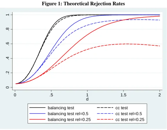
In Figure 1, we plot the power functions for both tests for three di¤erent magnitudes of the measurement error. The …rst set involves the power functions with no measurement error. The power functions can be seen to increase quickly with d, and both tests reject with virtual certainty as d reaches values of 1. The balancing test is slightly more powerful but this di¤erence is small, and only visible in the …gure for a small range of d:

The second set of power functions corresponds to a reliability ratio forxm i

of = 0:5. Measurement error of that magnitude visibly a¤ects the power of both tests. The balancing test still rejects with certainty for d > 1:5 while the power the coe¢ cient comparison test ‡attens out around a value of 0.93. This discrepancy becomes even more pronounced with a = 0:25. The power of the coe¢ cient comparison test does not rise above 0.6 in this case, while the balancing test still rejects with a probability of 1 at values of d slightly above 2.3

The results in Figure 1 highlight two important things. There are para-meter combinations where the balancing test has substantially more power 3_{Power for the cc test can actually be seen to start to decline as d increases. This} comes from the fact that the amount of measurement error is parameterized in terms of the reliability of xm_i . For a constant reliability the amount of measurement error increases withd. We felt that thinking about the reliability is probably the most natural way for applied researchers to think about the amount of measurement error they face in a variable.

than the coe¢ cient comparison test. On the other hand, there are other regions where the power of the two tests is very similar, for example, the region where d < 0:5 in Figure 1. In these cases, both tests perform very similar but, of course, speci…c results may di¤er in small samples. Hence, in a particular application, the coe¢ cient comparison test may reject when the balancing test doesn’t.

The homoskedastic case with classical measurement error might be highly stylized and not correspond well to the situations typically encountered in empirical practice. We therefore explore some other scenarios as well using simulations. Figure 2 shows the original theoretical power functions for the case with no measurement error from Figure 1. It adds empirical rejection rates from simulations with heteroskedastic errors ui and ei of the form

2

u;i =

ejsij

1 +ejsij

2 2 0u

2

e;i =

ejsij

1 +ejsij

2 2 0e:

We chose the baseline variances 20u and 20e so that 2u = 3 and 2e = 30 to

match the variances in Figure 1. All test statistics employ robust standard errors. We plot the rejection rates for data with no measurement error and for the more severe measurement error given by a reliability ratio = 0:25.4 As can be seen in Figure 2, both the balancing and the coe¢ cient comparison tests lose some power when the residuals are heteroskedastic compared to the homoskedastic baseline. Otherwise, the results look very similar to those in Figure 1. Heteroskedasticity does not seem to alter the conclusions appreciatively.

Next, we explore mean reverting measurement error (Bound et al., 1994). We generate measurement error as

mi = xi+ i

where is a parameter and Cov(xi; i) = 0, so that xi captures the error

related to xi and i the unrelated part. We set = 0:5 . Notice that xmi

4_{We did 25,000 replications in these simulations, and the underlying regressions have} a 100 observations.

can now be written as

xm_i = (1 + ) 0+ (1 + ) si+ (1 + )ui+ i;

so that this parameterization directly a¤ects the coe¢ cient in the balancing regression, which will be smaller than for a negative . At the same time, the residual variance in this regression is also reduced for a given reliabil-ity ratio.5 Figure 3 demonstrates that the power of both tests deteriorates even for moderate amounts of measurement error now but the coe¢ cient comparison test is still most a¤ected.

The case of mean reverting measurement error captures a variety of ideas, including the one that we may observe only part of a particular concept. Imagine we would like to include in our regression a variablexi =w1i+w2i,

where w1i and w2i are two orthogonal variables. We observe xmi = w1i. For

example, xi may be family background, w1i is mother’s education and other

parts of family background correlated with it, and w2i are all relevant parts

of family background, which are uncorrelated with mother’s education. As long as selection bias due to w1i and w2i is the same, this amounts to the

mean reverting measurement error formulation above. This scenario is also isomorphic to the model studied by Oster (2015). See the appendix for details.

5

Empirical Analysis

We illustrate the theoretical results in the context of estimating the returns to schooling using data from the National Longitudinal Survey of Young Men. This is a panel study of about 5,000 male respondents interviewed from 1966 to 1981. The data set has featured in many prominent analyses of the returns to education, including Griliches (1977) and Card (1995). We

5_{Note that …xing ,} 2 _{is given by}

2 ₌1 (1 + )_{V ar(x} i):

use the NLS extract posted by David Card and augment it with the variable on body height measured in the 1973 survey. We estimate regressions similar to eq. (2). The variableyi is the log hourly wage in 1976 andsi is the number

of years of schooling reported by the respondent in 1976. Our samples are restricted to observations without missing values in any of the variables used in a particular table or set of tables.

We start in Table 2 by presenting simple OLS regressions controlling for experience, race, and region of residence. The estimated return to schooling is 7.5%. This estimate is unlikely to re‡ect the causal e¤ect of education on income because important confounders, which in‡uence both education and income simultaneously such as ability or family background, are not controlled for.

In columns (2) to (5) we include variables which might proxy for the re-spondent’s family background. In column (2) we include mother’s education, in column (3) whether the household had a library card when the respondent was 14, and in column (4) we add body height measured in inches. Each of these variables is correlated with earnings and the coe¢ cient on education moves moderately when these controls are included. Mother’s education captures an important component of a respondent’s family background. The library card measure has been used by researchers to proxy for important parental attitudes (e.g. Farber and Gibbons, 1996). Body height is a vari-able determined by parents’genes and by nutrition and disease environment during childhood. It is unlikely a particularly powerful control variable but it is predetermined and correlated with family background, self-esteem, and ability (e.g. Persico, Postlewaite, and Silverman, 2004; Case and Paxson, 2008). The return to education falls by .1 to .2 log points when these con-trols are added. In column (5) we enter all three variables simultaneously. The coe¢ cients on the controls are somewhat attenuated and the return to education falls slightly further to 7.1%.

It might be tempting to conclude from the relatively small change in the estimated returns to schooling that this estimate might safely be given a causal interpretation. We provide a variety of evidence that this conclusion

is unlikely to be a sound one. Below the estimates in columns (2) to (5), we display the p-values from the coe¢ cient comparison test, comparing each of the estimated returns to education to the one from column (1). Although the coe¢ cient movements are small, the tests all reject at the 5% level, and in columns (4) and (5) they reject at the 1% level.

The results in columns 6 to 8, where we regress maternal education, the library card, and body height on education demonstrates this worry. The ed-ucation coe¢ cient is positive and strongly signi…cant in all three regressions, with t-values ranging from 4.4 to 13.1. The magnitudes of the coe¢ cients are substantively important. It is di¢ cult to think of these results as causal e¤ects: the respondent’s education should not a¤ect predetermined proxies of family background. Instead, these estimates re‡ect selection bias. Individ-uals with more education have signi…cantly better educated mothers, were more likely to grow up in a household with a library card, and experienced more body growth when young. Measurement error leads to attenuation bias when these variables are used on the right-hand side which renders them fairly useless as controls. The measurement error does not matter for the estimates in columns 6-8, and these are informative about the role of selection. Com-paring the p-values at the bottom of the table to the corresponding ones for the coe¢ cient comparison test in columns 2 to 4 demonstrates the superior power of the balancing test.

Finally, we report a number of additional results in the table. The R2 from regression of education on the added regressor (mother’s education, the library card, or height) is an ingredient necessary for the calculations that follow. Next, we report the values for if the added regressor was the only remaining source of omitted variables bias, assuming various degrees of measurement error. These calculations are based on equation (11). Since the idea that any of the candidate controls by themselves would identify the return in these bare bones wage equations does not seem particularly believable we will discuss these results in the context of Table 3.

In Table 3 we repeat the same set of regressions including a direct measure for ability, the respondent’s score on the Knowledge of the World of Work

test (KWW), a variable used by Griliches (1977) as a proxy for ability. The sample size is reduced due to the exclusion of missing values in the test score. Estimated returns without the KWW score are very similar to those in the original sample. Adding the KWW score reduces the coe¢ cient on education by almost 20%, from 0.075 to 0.061. Adding maternal education, the library card, and body height does very little now to the estimated returns to education. The coe¢ cient comparison test indicates that none of the small changes in the returns to education are signi…cant. Controlling for the KWW scores has largely knocked out the library card e¤ect but done little to the coe¢ cients on maternal education and body height. The relatively small and insigni…cant coe¢ cient movements in columns (2) to (5) suggest that the speci…cation controlling for the KWW score might solve the ability bias problem.

Columns (6)-(8), however, show that the regressions with the controls on the left hand side still mostly result in signi…cant education coe¢ cients even when the KWW score is in the regression. This suggests that the estimated returns in columns 1-5 might also still be biased by selection. The estimated coe¢ cients on education for the three controls are on the order of half their value from Table 1, and the body height measure is now only signi…cant at the 10% level. Particularly the relationship between mother’s and own education is still sizable, and this measure still indicates the possibility of important selection.

The calculations at the bottom of the table based on equation (11) also con…rm that mother’s education might potentially pick up variation due to an important confounder. These calculations assume that mother’s education is the only omitted control in column (1) while acknowledging that the available measure might contain a lot of noise compared to the correct control. With the moderate amounts of measurement error implied by a reliability of 0.75 or 0.5 the returns to education coe¢ cient still moves fairly little when adding mother’s education. For a reliability of 0.5 the return remains .058 compared to .061 without controlling for mother’s education. If the reliability is only 0.25 the return falls more strongly to 0.055. In order for the entire estimated

return in column (1) to be explained by omitted variables bias due to mother’s education the reliability needs to be as low as 0.05, as can be seen in the last row.

These numbers highlight a lot of curvature in the relationship between the reliability and the implied return to education. Figure 4 illustrates this for the case of the mother’s education variable. It becomes clear that the return changes little for reliabilities above 0.25 but then falls precipitously for more severe measurement error. If we believe that mother’s education captures family background poorly enough there is a lot room for bias from this source.

Looking at the columns (3) and (4) we can see that the same isn’t true for the library card and body height measures. Here the returns relationship is essentially ‡at over the range of reliabilities as low as 0.25. Reliabilities as low as 0.01 are necessary for a zero return. This con…rms that these variables have lost most of their power as confounders once KWW is controlled in the regressions. The ‡at relationship between the reliability and returns is due to the fact that both and m are lower for the library card and body height in Table 3 compared to Table 2. We don’t claim here that adding these variables to the regressions with the KWW score would be a suitable identi…cation strategy in any case. Rather, we see the implied calculation for di¤erent reliabilities as an intuitive measure summarizing the impact of the relevant values of , m_{, and the R}2 _{between years of education and the} added regressor.

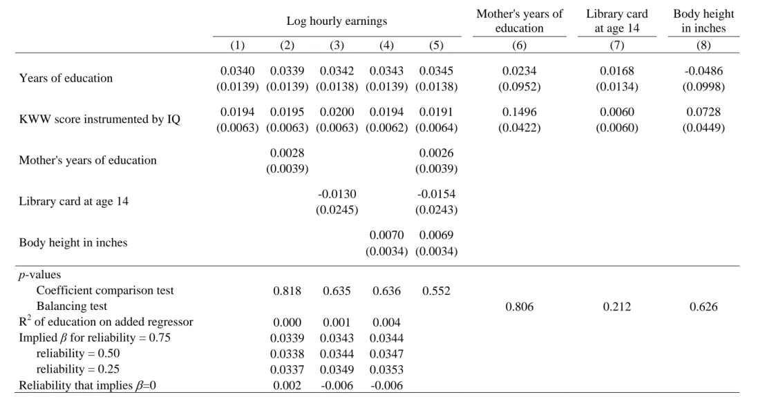
While the KWW score might be a powerful control it is likely also mea-sured with substantial error. Griliches (1977) proposes to instrument this measure with an IQ testscore variable, which is also contained in the NLS data, to eliminate at least some of the consequences of this measurement er-ror. In Table 4 we repeat the schooling regressions with IQ as instrument for the KWW score. The coe¢ cient on the KWW score almost triples, in line with the idea that an individual test score is a very noisy measure of ability. The education coe¢ cient now falls to only about half its previous value from 0.061 to 0.034. This might be due to positive omitted variable bias present

in the previous regressions which is eliminated by IQ-instrumented KWW (although there may be other possible explanations for the change as well). Both the coe¢ cient comparison tests and the balancing tests indicate no ev-idence of selection any more. This is due to a combination of lower point estimates and larger standard errors. The contrast between tables 3 and 4 highlights the usefulness of the balancing test: it warns about the Table 3 results, while the coe¢ cient comparison test delivers insigni…cant di¤erences in either case.

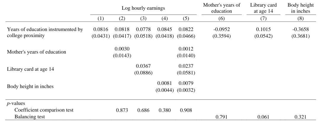
Finding an instrumental variable for education is an alternative to con-trol strategies, such as using test scores. In Table 5 we follow Card’s (1995) analysis and instrument education using distance to the nearest college, while dropping the KWW score.6 _{We use the same sample as in Table 2, which} di¤ers from Card’s sample.7 _{Our IV estimates of the return to education are} slightly higher than in Table 2 but a lot lower than in Card (1995) at around 8%. The IV returns estimates are noisy, never quite reaching a t-statistic of 2. Columns 1-5 of Table 5 show that the IV estimate on education, while bouncing around a bit, does not change signi…cantly when maternal edu-cation, the library card, or body height are included. In particular, if these three controls are included at the same time in column (5) the point estimate is clearly indistinguishable from the unconditional estimate in column (1).

IV regressions with pre-determined variables on the left hand side can be thought of as a test for the exclusion restriction or random assignment of the instruments. Unfortunately, in this case the selection regressions in columns (6)-(8) are also much less precise and as a result less informative. The coe¢ cients in the regressions for mother’s education and body height have the wrong sign but con…dence intervals cover anything ranging from zero selection to large positive amounts. Only the library card measure is large, positive, and signi…cant around the 6% level, warning of some remaining potential for selection even in the IV regressions. While the data do not 6_{We use a single dummy variable for whether there is a four year college in the county,} and we instrument experience and experience squared by age and age squared.

7_{We restrict Card’s sample to non-missing values in maternal education, the library} card, and body height.

speak clearly in this particular case this does not render the methodology any less useful.

6

Conclusion

Using predetermined characteristics as dependent variables o¤ers a useful speci…cation check for a variety of identi…cation strategies popular in empiri-cal economics. We argue that this is the case even for variables which might be poorly measured and are of little value as control variables. Such vari-ables should be available in many data sets, and we encourage researchers to perform such “balancing” tests more frequently. We show that this is a more powerful strategy than adding the same variables on the right hand side of the regression as controls and looking for movement in the coe¢ cient of interest.

We have illustrated our theoretical results with an application to the returns to education. Taking our assessment from this exercise at face value, a reader might conclude that the results in Table 4, returns around 3.5%, can safely be regarded as causal estimates. Of course, this is not the conclusion reached in the literature, where much higher IV estimates like those in Table 5 are generally preferred (see e.g. Card, 2001 or Angrist and Pischke, 2015, chapter 6). This serves as a reminder that the discussion here is focused on sharpening one particular tool in the kit of applied economists; it is not a miracle cure for all ills.

The balancing test and other statistics we discuss here are useful to gauge selection bias due to observed confounders, even when they are potentially measured poorly. It does not address any other issues which may also haunt a successful empirical investigation of causal e¤ects. One possible issue is measurement error in the variable of interest, which is also exacerbated as more potent controls are added. Griliches (1977) shows that a modest amount of measurement error in schooling may be responsible for the patterns of returns we have displayed in Tables 2 to 4. Another issue, also discussed by Griliches, is that controls like test scores might themselves at least be

partly in‡uenced by schooling, which would make them bad controls. For all these reasons, IV estimates of the returns may be preferable.

There are other issues we have sidestepped in our analysis. Our discus-sion has focused on the case where a researcher has a single regressor or a small set of such regressors available for addition to a candidate regression. But sometimes we might be interested in the robustness of the original re-sults when a large number of regressor are added. An example would be a di¤erences-in-di¤erences analysis in a state-year panel, where the researcher is interested in checking whether the results are robust to the inclusion of state speci…c trends. The balancing test seems to be of little use in this case. In fact, the analysis in Hausman (1978) and Holly (1982) highlights that the coe¢ cient comparison (Hausman) test may be particularly powerful in some cases where many regressors are added.8 _{Whether the principles of} the balancing test can be harnessed in a fruitful way for such scenarios is a useful avenue for future research.

References

[1] Angrist, Joshua and Jörn-Ste¤en Pischke (2015)Mastering Metrics. The Path from Cause to E¤ect, Princeton: Princeton Univeristy Press.

[2] Altonji, Joseph G., Timothy Conley, Todd E. Elder, and Christopher R. Taber (2013) “Methods for Using Selection on Observed Variables to Address Selection on Unobserved Variables,” mimeographed.

[3] Altonji, Joseph G., Todd E. Elder, and Christopher R. Taber (2005) “Selection on Observed and Unobserved Variables: Assessing the E¤ec-tiveness of Catholic Schools,”Journal of Political Economy, vol. 113, no. 1, Februrary, 151-184.

[4] Battistin, Erich and Andrew Chesher (2014), “Treatment E¤ect Esti-mation with Covariate Measurement Error,”Journal of Econometrics, vol 178, no. 2, February, 707-715.

[5] Bound, John et al. (1994) “Evidence on the Validity of Cross-Sectional and Longitudinal Labor Market Data,”Journal of Labor Economics, vol. 12, no. 3, 345-368.

[6] Card, David (1995) “Using Geographic Variations in College Proximity to Estimate the Returns to Schooling,” in Aspects of Labor Market Be-havior: Essays in Honor of John Vanderkamp, L. N. Christo…des, E. K. Grand, and R. Swidinsky, eds., Toronto: University of Toronto Press.

[7] Card, David (2001) “Estimating the Return to Schooling: Progress on Some Persistent Econometric Problems,”Econometrica, vol. 69, Sep-tember, 1127–1160.

[8] Case, Anne, and Christina Paxson (2008) “Stature and Status: Height, Ability, and Labor Market Outcomes, ”Journal of Political Economy, vol. 116, no. 3, 499-532.

[9] Farber, Henry S., and Robert Gibbons (1996) “Learning and Wage Dy-namics,”The Quarterly Journal of Economics, vol. 111, no. 4, 1007-1047.

[10] Gelbach, Jonah B. (2009) “When Do Covariates Matter? And Which Ones, and How Much?”University of Arizona Department of Economics Working Paper #09-07.

[11] Griliches, Zvi (1977) “Estimating the Returns to Schooling - Some Econometric Problems,”Econometrica, vol. 45, January, 1-22.

[12] Hausman, Jerry (1978) “Speci…cation Tests in Econometrics,” Econo-metrica, vol. 46, no. 6, November, 1251-1272.

[13] Holly, Alberto (1982) “A Remark on Hausman’s Speci…cation Test,”

Econometrica, vol. 50, no. 3, May, 749-759.

[14] Imbens, Guido W. (2003) “Sensitivity to Exogeneity Assumptions in Program Evaluation,”American Economic Review Papers and Proceed-ings, vol. 93, no. 2, May, 126-132.

[15] MacKinnon, James G. (1992) “Model Speci…cation Tests and Arti…cial Regressions,”Journal of Economic Literature, vol. 30, no. 1, March, 102-146.

[16] Oster, Emily (2015) “Unobservable Selection and Coe¢ cient Stability: Theory and Evidence,” mimeographed, Brown University, January 26.

[17] Persico, Nicola, Andrew Postlewaite and Dan Silverman (2004) “The E¤ect of Adolescent Experience on Labor Market Outcomes: The Case of Height,”Journal of Political Economy, vol. 112, no. 5, 1019-1053.

[18] Rosenbaum, Paul R. and Donald B. Rubin (1983) “Assessing Sensitivity to an Unobserved Binary Covariate in an Observational Study with Bi-nary Outcome,”Journal of the Royal Statistical Society. Series B, vol. 45, no. 2, 212-218.

Figure 1: Theoretical Rejection Rates

Figure 2: Simulated Rejection Rates with Heteroskedasticity

Note: The black lines are theoretical power functions for the homoskedastic case with conventional standard errors, the blue and red and lines are simulated rejection rates with heteroskedastic errors and robust standard errors.

0

.2

.4

.6

.8

1

0 .5 1 1.5 2

d

balancing test cc test balancing test rel=0.5 cc test rel=0.5 balancing test rel=0.25 cc test rel=0.25

0

.2

.4

.6

.8

1

0 .5 1 1.5 2

d

power fct. bal. test power fct. cc test rej. rate bal. test rej. rate cc test

29

Figure 3: Simulated Rejection Rates with Mean Reverting Measurement Error

Note: The black lines are theoretical power functions with classical measurement error and conventional standard errors, the blue and red and lines are simulated rejection rates with mean reverting measurement error and robust standard errors.

Figure 4: Implied



0

.2

.4

.6

.8

1

0 .5 1 1.5 2

d

power fct. bal. test power fct. cc test rej. rate bal. test rel=.75 rej. rate cc test rel=.75 rej. rate bal. test rel=.5 rej. rate cc test rel=.5

0

.0

2

.0

4

.0

6

be

ta

0 .2 .4 .6 .8 1

Table 1: Parameters for Power Calculations and Implied R2s

1



3 n = 100

30 d

R2

 =

 =

 =

0 0.47 0.24 0.12

0.5 0.49 0.26 0.15 1.0 0.55 0.31 0.22 1.5 0.61 0.39 0.32 2.0 0.68 0.47 0.42

31

Table 2: Baseline Regressions for Returns to Schooling and Specification Checks

Log hourly earnings Mother's years of education

Library card at age 14

Body height in inches

(1) (2) (3) (4) (5) (6) (7) (8)

Years of education 0.0751 0.0728 0.0735 0.0740 0.0710 0.3946 0.0371 0.1204

(0.0040) (0.0042) (0.0040) (0.0040) (0.0042) (0.0300) (0.0040) (0.0273)

Mother's years of education 0.0059 0.0044

(0.0029) (0.0030)

Library card at age 14 0.0428 0.0361

(0.0183) (0.0184)

Body height in inches 0.0090 0.0084

(0.0027) (0.0027)

p-values

Coefficient comparison test 0.045 0.023 0.010 0.002

Balancing test 0.000 0.000 0.000

R2 of education on added regressor 0.073 0.032 0.007 Implied β for reliability = 0.75 0.0719 0.0730 0.0737

reliability = 0.50 0.0700 0.0718 0.0729

reliability = 0.25 0.0628 0.0680 0.0707

Reliability that implies



N = 2,500 in all regressions. Heteroskedasticity robust standard errors in parentheses. All regressions control for experience, experience-squared, indicators for black, for southern residence and residence in an SMSA in 1976, indicators for region in 1966 and living in an SMSA in 1966.

Table 3: Regressions for Returns to Schooling and Specification Checks Controlling for the KWW Score

Log hourly earnings Mother's years of education

Library card at age 14

Body height in inches

(1) (2) (3) (4) (5) (6) (7) (8)

Years of education 0.0609 0.0596 0.0608 0.0603 0.0591 0.2500 0.0133 0.0731

(0.0059) (0.0060) (0.0059) (0.0059) (0.0060) (0.0422) (0.0059) (0.0416)

KWW score 0.0070 0.0068 0.0069 0.0069 0.0067 0.0410 0.0076 0.0145

(0.0015) (0.0016) (0.0016) (0.0015) (0.0016) (0.0107) (0.0016) (0.0117)

Mother's years of education 0.0053 0.0048

(0.0037) (0.0037)

Library card at age 14 0.0097 0.0045

(0.0215) (0.0216)

Body height in inches 0.0078 0.0075

(0.0034) (0.0034)

p-values

Coefficient comparison test 0.163 0.652 0.158 0.085

Balancing test 0.000 0.025 0.079

R2 of education on added regressor 0.033 0.006 0.002 Implied β for reliability = 0.75 0.0591 0.0607 0.0602

reliability = 0.50 0.0582 0.0607 0.0598

reliability = 0.25 0.0550 0.0604 0.0586

Reliability that implies



N = 1,773 in all regressions, due to missing values in IQ. Heteroskedasticity robust standard errors in parentheses. All regressions control for experience, experience-squared, indicators for black, for southern residence and residence in an SMSA in 1976, indicators for region in 1966 and living in an SMSA in 1966.

33

Table 4: Regressions for Returns to Schooling and Specification Checks Instrumenting the KWW Score

Log hourly earnings Mother's years of education

Library card at age 14

Body height in inches

(1) (2) (3) (4) (5) (6) (7) (8)

Years of education 0.0340 0.0339 0.0342 0.0343 0.0345 0.0234 0.0168 -0.0486 (0.0139) (0.0139) (0.0138) (0.0139) (0.0138) (0.0952) (0.0134) (0.0998) KWW score instrumented by IQ 0.0194 0.0195 0.0200 0.0194 0.0191   0.1496   0.0060   0.0728

(0.0063) (0.0063) (0.0063) (0.0062) (0.0064)   (0.0422)   (0.0060)   (0.0449)

Mother's years of education    0.0028       0.0026               

   (0.0039)       (0.0039)               

Library card at age 14       -0.0130    -0.0154               

      (0.0245)    (0.0243)               

Body height in inches          0.0070 0.0069               

         (0.0034) (0.0034)               

p-values

Coefficient comparison test 0.818 0.635 0.636 0.552

Balancing test      0.806   0.212   0.626

R2 of education on added regressor 0.000 0.001 0.004 Implied β for reliability = 0.75 0.0339 0.0343 0.0344

reliability = 0.50 0.0338 0.0344 0.0347

reliability = 0.25 0.0337 0.0349 0.0353

Reliability that implies



N = 1,773 in all regressions, due to missing values in IQ. Heteroskedasticity robust standard errors in parentheses. All regressions control for experience, experience-squared, indicators for black, for southern residence and residence in an SMSA in 1976, indicators for region in 1966 and living in an SMSA in 1966.

Table 5: Regressions for Returns to Schooling and Specification Checks Instrumenting Schooling by Proximity to College

Log hourly earnings Mother's years of education

Library card at age 14

Body height in inches

(1) (2) (3) (4) (5) (6) (7) (8)

Years of education instrumented by college proximity

0.0816 0.0818 0.0778 0.0845 0.0822 -0.0952 0.1015 -0.3658 (0.0431) (0.0417) (0.0518) (0.0418) (0.0466) (0.3594) (0.0542) (0.3681)

Mother's years of education    0.0030       0.0012               

   (0.0143)       (0.0140)               

Library card at age 14       0.0367    0.0237               

      (0.0886)    (0.0581)               

Body height in inches          0.0081 0.0079               

         (0.0044) (0.0032)               

p-values

Coefficient comparison test 0.873 0.686 0.380 0.908

Balancing test      0.791   0.061   0.321

N = 2,500 in all regressions. Heteroskedasticity robust standard errors in parentheses. All regressions control for experience, experience-squared, indicators for black, for southern residence and residence in an SMSA in 1976, indicators for region in 1966 and living in an SMSA in 1966.

7

Appendix

7.1

Power Functions

xi = 0+ si+ ui;

however, xi is measured with error

xm_i =xi+mi:

E¤ectively, we run the balancing regression

xm_i = m₀ + msi+ ui+mi:

The test statistic for the null hypothesis that the balancing coe¢ cient is zero is

t m = bm se bm

= b

m

1

p_n

p ₂

u+ 2m s

De…ne

=

2 m 2 u+ 2m

) 2u+

2

m =

2 u

1 Hence

t m =b

mpn _sp1 u

The rejection probability is

Pr (_jt mj> CjH₁) = Pr (t m > CjH₁) + Pr (t m < CjH₁)

= Pr

0

@ b

m

se bm

> C H1 1

A+ Pr

0

@ b

m

se bm

< C H1 1 A = Pr 0 @ b m d se bm

> C d p n s p 1 u H1 1 A + Pr 0 @ b m d se bm

< C p n s p 1 u H1 1 A d

!1 C d

p n s

p

1

u

+ C d p

n s

p

1

u

This is the power function of the balancing test

P owert (d) = 1 1:96 d

p n s

p

1

u

+ 1:96 d p n s p 1 u :

7.1.2 The Coe¢ cient Comparison Test The short and long regressions are

yi = s+ ssi+esi yi = + si+ xi+ei;

and

xi = 0+ si+ ui:

Adding measurement error in xi:

xm_i =xi+mi;

we have

yi = s+ ssi+esi

yi = m+ msi+ mxmi +e m i xm_i = 0+ si+ ui+mi:

Treatsi, ui,ei, and mi as the underlying disturbances which in turn will

xi, it follows that Cov(ei; ui) = 0. We normalize si to a mean zero variable. Hence, si ui ei mi 0 B B @ 2 6 6 4 0 0 0 0 3 7 7 5; 2 6 6 4

s 0 0 0

0 u 0 0

0 0 e 0

0 0 0 m 3 7 7 5 1 C C A:

We want to test s m= 0. Of course

s m

= m;

and we will assume ₆= 0, so that

s m _{= 0}

, = 0:

The test statistic is

t = b

s bm r

V ar bs +V ar bm 2Cov bs;bm ;

which is asymptotically standard normal. The sampling variances are

V ar bm = 1

n

V ar(em i ) V ar(_esm

i )

V ar bs = 1

n

V ar(es_i)

2 s

;

which we will now derive in terms of the underlying parameters. We start by derivingV ar bm . _esm

i is given by si = 0+ 1xmi +se

m i

and

V ar(xm_i ) = 2 2_s+ 2_u+ 2_m

Cov(xm_i ; si) = 2s

so

2

s =

2

1V ar(x m

i ) +V ar(es m i ) 2

s =

Cov(xm i ; si)2 V ar(xm

i )

2 V ar(x m

i ) +V ar(es m i ) = 2 4 s 2 ₂

s+ 2u+ 2m

+V ar(_esm_i )

V ar(s_em_i ) =

2

s( 2u+ 2m) 2 ₂

Next, we needV ar(em

i ). De…ne the reliability

= V ar(xi)

V ar(xm i )

=

2 2 s+ 2u 2 2

s+ 2u+ 2m

and the R2 _{of the regression of s}

i onxmi R2 = 1 V ar(es

m i ) 2 s = 1 2 u+ 2m 2 ₂

s + 2u+ 2m

=

2 2 s 2 ₂

s + 2u+ 2m ;

Then

m

= + 1 1 R2

= +

2 m 2 2

s+ 2u+ 2m 2 u+ 2m 2 2

s+ 2u+ 2m

= +

2 m 2 u+ 2m

;

and

m

= R

2

1 R2

=

2 u 2 2

s+ 2u+ 2m 2 u+ 2m 2 2

s+ 2u+ 2m

=

2 u 2 u+ 2m

: Using = 2 m 2 u+ 2m

we have

m

= +

m _{= (1 )}

Using these results in

yi = m+ msi+ mxmi +e m i

= m+ ( + )si+ (1 )xmi +e m i

= ( m+ (1 ) 0) + ( + )si+ (1 ) (ui+mi) +emi yi = + si+ ( 0+ si+ ui) +ei

Matching residuals yields

ui+ei = (1 ) (ui+mi) +emi em_i = ui (1 )mi +ei V ar(em_i ) = 2 2 2_u+ 2(1 )2 2_m+ 2_e

= 2

2 m 2 u+ 2m

2 2 u+ 2 u 2 u+ 2m

2 2 m

!

+ 2_e = 2 2_u+ 2_e

So

V ar bm = 1

n

V ar(em i ) V ar(_esm

i )

= 1

n

2 2

u+ 2e 2

s( 2u+ 2m) 2 2

s+ 2u+ 2m

= 1

n

2_{(1 )}

2 u + 1 2 s 2 2 u+ 2 e

and similarly we can derive

V ar(_bm) = 1

n

V ar(em i ) V ar(x_em

i )

= 1

n

2 2

u+ 2e 2

u+ 2m

= 1 n 2 ₊ 2 e 2 u

Now we derive V ar bs , which does not involve the mismeasured xi.

Comparing the short and the long regression, the relationship between the residuals is

yi = s+ ssi+esi

= s+ ( + )si+esi

yi = + si+ ( 0+ si+ ui) +ei

= + 0+ ( + )si+ ui+ei es_i = ui+ei;

and hence

so

V ar bs = 1

n

V ar(es i) 2 s = 1 n 2 2

u+ 2e 2 s

:

Finally, we deriveCov bs;b . Using

bs s ₌

P es

isi P

s2 i

bm m

=

P em

i esmi P

(_esm i ) 2 we have p n P es_isi P

em i esmi

d

!N 0; E (e

s i)

2

s2_i E[es_iem_i siesmi ] E[es_iem_i siesmi ] E (emi )

2

(_esm_i )2 : In addition, using

plim 1

n X

s2_i = 2_s

plim 1

n X

(_esm_i )2 = V ar(_esm_i );

by Slutsky’s theorem

Cov bs;b = 1

n E[es

iemi siesmi ] 2

sV ar(esmi )

= 1

n

E[E(es_iem_{i j}si;esmi )siesmi ] 2

sV ar(esmi )

= 1

n

Cov(es

i; emi )V ar(esmi ) 2

sV ar(esmi )

= 1

n

Cov(es_i; em_i )

2 s

:

Using our earlier result that

yi = ( m+ (1 ) 0) + ( + )si+ (1 ) (ui+mi) +emi

and comparing this to the short regression

yi = s+ ssi+esi;

we have

Note that ui+mi is the residual from a regression ofxmi onsi, we have Cov(es_i; em_i ) =V ar(em_i ) = 2 2_u+ 2_e

and hence

Cov bs;bm = 1

n

2 2

u+ 2e 2 s

:

Returning to the test statistic

t = b

s bm r

V ar bs +V ar bm 2Cov bs;bm

we …rst derive 1

nV (d; ) = V ar b s

+V ar bm 2Cov bs;bm

= 1

n 2 2

u+ 2e 2 s

+ 1

n 2 2

s+ 2u+ 2m 2

s( 2u+ 2m)

2 2 u+ 2 e 2 1 n 2 2

u+ 2e 2 s

= 1

n

( 2_{(1 2 )} 2

u 2e) ( 2u+ 2m) + 2 2

s+ 2u+ 2m ( 2 2u+ 2e) 2

s( 2u + 2m)

!

= 1

n(1 )

2 2 u 2 s

+ 2 2+

2 2 e 2 u

Note that

s m ₌ m _{= (1 )}

so the power function of the coe¢ cient comparison test is

P owert (d; ) = 1 1:96 d

p

n (1 )

p

V (d; )

!

+ 1:96 d p

n (1 )

p

V (d; )

! :

7.2

Comparison with Oster (2015)

Oster’s (2015) formulation of the causal regression takes the form

yi = + si+ w1i+w2i+ei;

where w1i is an observed covariate and w2i is an unobserved covariate,

un-correlated with w1i. To map this into our setup, think of the true xi as

capturing both w1i andw2i, i.e. xi = w1i+w2i. Furthermore, there is equal

selection, i.e.

Cov(si; w1i) 2 2

1

= Cov(si₂; w2i)

2 ;

where 2

1 and 22 are the variances of w1i andw2i, respectively. Then, Oster’s

regression can be written as

yi = + si+xi+ei;

which is our regression with = 1 (the scaling of xi is arbitrary of course; it

could be xi =w1i+w2i= instead and = or anything else).

Our observedxm_i = w1i, so measurement errormi = w2i. Measurement

error here is mean reverting, i.e.

mi = xi+ i: (A1)

Notice that

Cov(mi; xi) = 22

and hence

=

2 2 2 2

1+ 22

(A2) and

i = w2i ( w1i+w2i)

= w1i (1 + )w2i

=

2 2 2 2

1+ 22 w1i

2 2 1 2 2

1+ 22 w2i:

It turns out that _i implicitly de…ned in (A1) and the given by (A2) satisfy

Cov(xi; i) = 0 and Cov(si; i) = 0. Hence, these two equations represent

mean reverting measurement error as de…ned in the body of the manuscript. However, note that Cov(si; i) = 0 depends on the equal selection

assump-tion. With proportional selection, i.e.

Cov(si; w1i) 2 2

1

= Cov(si₂; w2i)

2 ;