If Technology has Arrived Everywhere, why Has Income Diverged?

If Technology has Arrived Everywhere,

why Has Income Diverged?

Diego Comin

Harvard University and NBER

Mart´ı Mestieri

Toulouse School of Economics May 1, 2014∗

Abstract

We study the cross-country evolution of technology diffusion processes. Using data from the last two centuries for twenty-five major technologies, we document two new facts: there has been convergence in adoption lags between rich and poor countries, while there has been divergence in long run penetration rates, once technologies are adopted. We show that the evolution of aggregate productivity implied by these trends in technology diffusion accounts for the bulk of the evolution of the world income distribution in the last two hundred years. In particular, initial cross-country differences in adoption lags account for a significant part of the cross-country income divergence in the nineteenth century. The divergence in penetration rates accounts for the divergence during the twentieth century.

Keywords: Technology Diffusion, Transitional Dynamics, Great Divergence. JEL Classification: E13, O14, O33, O41.

∗

This paper subsumes two earlier working papers circulated under the title “An Intensive Exploration of Technology Adoption” and “If Technology Has Arrived Everywhere, Why Has Income Diverged?.” We are grate-ful to Thomas Chaney, Gino Gancia, Christian Hellwig, Chad Jones, Pete Klenow, Franck Portier, Mar Reguant, Doug Staiger, Jon Van Reenen and seminar participants at Aix-Marseille, Boston University, Brown, CERGE-EI, Dartmouth, Edinburgh, HBS, Harvard, LBS, Minnesota Fed, Pompeu Fabra, Stanford GSB, Aut`onoma de Barcelona, University of Toronto, TSE and the World Bank for useful comments and suggestions. Comin acknowledges the generous support of INET and the NSF. Mestieri acknowledges the generous support of the ANR. All remaining errors are our own. Comin: dcomin@hbs.edu, Mestieri: marti.mestieri@tse-fr.eu

1

Introduction

At the beginning of the nineteenth century, differences in income per capita between rich and poor countries were relatively small. The average income per capita in 1820 of the seventeen advanced countries denoted by Maddison (2004) as “Western countries” was 1.9 times the average of non-Western countries.1 For the next 180 years, Western countries grew signifi-cantly faster and, by 2000, their per capita income was 7.2 times the average of non-Western countries. This divergence in income is known as the Great Divergence (e.g., Pritchett,1997 and Pomeranz,2000), and is one of the great puzzles in economics (Acemoglu,2011).

More generally, we know little about the drivers of cross-country differences in productivity growth over protracted periods of time. For example,Klenow and Rodr´ıguez-Clare(1997) show that factor accumulation (physical and human capital) accounts only for 10% of cross-country differences in growth between 1960 and 1985. Clark and Feenstra(2003) find similar results for the period 1850-2000. What accounts for the bulk of cross-country differences in the evolution of productivity over long horizons and, in particular, for the Great Divergence?

This paper explores the role that technology has played in the evolution of income growth. To this end, we first study how technology has diffused over the last 200 years. We document significant differences in technology diffusion across countries. Second, we quantify the effect of these differential patterns of diffusion on the evolution of the world income distribution over the last two centuries.

We decompose the contribution of technology to productivity growth into the extensive and intensive margins. The extensive margin captures the range of technologies available, which is given by the lag with which new technologies are adopted. New technologies embody higher productivity. Therefore, a reduction in adoption lags increases the average productivity of technologies adopted, thereby raising aggregate productivity growth. The intensive margin captures the penetration rate of new technologies. The more units of any new technology (relative to income) a country uses, the higher the number of workers or units of capital that can benefit from the productivity gains brought by the new technology.2 As a result, increases in the penetration of technology raise the growth rate of productivity.

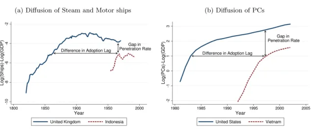
To study the evolution of technology diffusion, first we need to measure these adoption margins from the diffusion curves of individual technologies. We illustrate our strategy to identify the adoption margins in Figure 1. Figures 1a and 1b plot the (log) of the tonnage of steam and motor ships over real GDP in the UK and Indonesia and the (log) number of computers over real GDP for the U.S. and Vietnam, respectively. One feature of these plots is that, for a given technology, the diffusion curves for different countries have similar shapes,

1

Maddison(2004) defines as Western countries Austria, Belgium, Denmark, Finland, France, Germany, Italy, Netherlands, Norway, Sweden, Switzerland, Untied Kingdom, Japan, Australia, New Zealand, Canada and the United States.

Figure 1: Examples of diffusion curves

(a) Diffusion of Steam and Motor ships (b) Diffusion of PCs

but displaced vertically and horizontally. This property holds generally for a large majority of the technology-country pairs. Given the common curvature of diffusion curves, the relative position of a curve can be characterized by only two parameters. The horizontal shifter informs us about when the technology was introduced in the country. The vertical shifter captures the penetration rate the technology will attain when it has fully diffused.

These intuitions are formalized with a model of technology adoption and growth. Crucial for our purposes, the model provides a unified framework for measuring the diffusion of specific technologies and assessing their impact on income growth. The model features both adoption margins, and has predictions about how variation in these margins affect the curvature and level of the diffusion curve of specific technologies. This allows us to take these predictions to the data and estimate adoption lags and penetration rates fitting the diffusion curves derived from our model. We identify the extensive and intensive adoption margins for 25 significant technologies invented over the last 200 years for a sample of 130 countries. Then, we use our estimates to analyze the cross-country evolution of technology diffusion.

We document two new facts. First, cross-country differences in adoption lags have narrowed over the last 200 years. That is, adoption lags have declined more in poor/slow adopter countries than in rich/fast adopter countries. Second, the gap in penetration rates between rich and poor countries has widened over the last 200 years, inducing a divergence in the intensive margin of technology adoption. These patterns are consistent with Figure 1. The horizontal gap between the diffusion curves for steam and motor ships in the UK and Indonesia is much larger than the horizontal gap between the U.S. and Vietnam for computers (131 years vs. 11 years). In contrast, the vertical gap between the curves for ships in the UK and Indonesia are smaller than the vertical gap between the diffusion curves of computers in the U.S. and Vietnam (0.9 vs. 1.6).

After characterizing the patterns of technology diffusion, we evaluate quantitatively their implications for the evolution of the world income distribution. We estimate the evolution of the diffusion margins for various groups of countries. Then, we feed in the estimated diffusion patterns into the aggregate representation of our model economy, and we compare the resulting income dynamics with the data. Note that this approach does not force the estimated adoption margins to fit the actual aggregate productivity dynamics.

We find that initial cross-country differences in the patterns of technology diffusion induce a world income distribution that is very similar to the actual distribution in 1820. Cross-country differences in technology diffusion patterns over the last two centuries account well for the evolution of the world income distribution. The model generates very protracted transitional dynamics, which account better for the dynamics of productivity over longer horizons than the neoclassical growth model.3 Our simulations show that it took approximately one century since the beginning of the Industrial Revolution for Western economies to reach their Modern long run growth rate of 2%. With respect to the Great Divergence, we observe that differences in the evolution of technology diffusion induce an increase by a factor of 3.2 in the income gap between Western and non-Western countries between 1820 and 2000. This represents 82% of the actual increase in the income gap, which grew by a factor of 3.9.

It is important to emphasize that we use a general equilibrium model. Thus, when eval-uating the role of technology for cross-country differences in income, our analysis takes into account that income affects demand for goods and services that embody new technologies. In our baseline model, the restriction that our model has a balanced growth path implies that the income elasticity of technology demand is equal to one. Because this implication of the model may be restrictive, we assess the robustness of our findings to allowing for non-homotheticities in the demand for technology. That is, we allow the income elasticity of technology demand to differ from one. We find that our results are robust to allowing for non-homotheticities.

This paper is related to the literature analyzing the channels driving the Great Divergence. One stream of the literature has emphasized the role of the expansion of international trade during the second half of the nineteenth century. Galor and Mountford (2006) argue that trade affected asymmetrically the fertility decisions in developed and developing economies, due to their different initial endowments of human capital, leading to different evolutions of productivity growth. O’Rourke et al. (2012) elaborate on this perspective and argue that the direction of technical change, in particular the fact that after 1850 it became skill-biased (Mokyr,2002), contributed to the increase in income differences across countries, as Western countries benefited relatively more from them. Trade-based theories of the Great Divergence, however, need to confront two facts. Prior to 1850, the technologies brought by the Indus-trial Revolution were unskilled-biased rather than skilled-biased (Mokyr,2002). Yet, incomes

3_{See, for example, Barro and Sala-i-Martin (2003) and King and Rebelo (1993) for a calibration of the}

diverged also during this period. Second, trade globalization ended abruptly in 1913. With WWI, world trade dropped and did not reach the pre-1913 levels until the 1970s. In contrast, the Great Divergence continued throughout the twentieth century.

Probably motivated by these observations, another strand of the literature has studied the cross-country evolution of Solow residuals and has found that they account for the majority of the divergence (Easterly and Levine, 2001, and Clark and Feenstra, 2003). Though these authors interpret Solow residuals as a proxy for technology, our paper is the first to use direct measures of technology to document how technology diffusion patterns have evolved in the cross-section over the last two centuries. It is also the first to show the importance that these technology dynamics have had for cross-country income dynamics.4,5

Finally, our paper builds uponComin and Hobijn(2010). They estimate the adoption lags for 15 technologies and quantify how cross-country differences in average adoption lags con-tribute to differences in current income levels. To do this exercise, they assume all countries are in balanced growth path, growing at a common growth rate.6 In this paper, we develop a new procedure to estimate not only adoption lags, but also the intensive margin of adoption. In doing so, we build a multi-sectoral model that explicitly accounts for the complementar-ities across technologies. Second, we study for the first time the cross-country evolution of the intensive and extensive margins of technology adoption over the last two centuries. To our knowledge, we are the first to document the divergence of the intensive margin and the convergence of the adoption lags. Third, this paper studies the transitional dynamics of the model and, most importantly, how technology dynamics have contributed to the evolution of the world income distribution that we have observed over the last 200 years. As emphasized above, this is one of few papers that provides an account of the dynamics of income growth over protracted periods of time.

The rest of the paper is organized as follows. Section 2 presents the model. Section 3 presents the estimation strategy based on the structural model. Section 4 estimates the extensive and intensive margins of adoption and documents the cross-country evolution of both adoption margins. Section 5 quantifies the effect of the technology dynamics on the evolution of the world income distribution. Section 6concludes.

4_{Our analysis is also related to a strand of the literature that has studied the productivity dynamics after}

the Industrial Revolution. Crafts (1997),Galor and Weil(2000),Goodfriend and McDermott(1995),Hansen and Prescott(2002) andTamura(2002) among others, provide complementary reasons why there was a slow growth acceleration in productivity after the Industrial Revolution.

5

Our paper is also related toLucas(2000) who studies the evolution of the world income distribution using a model that assumes a negative relationship between the time a country takes off and the TFP growth it experiences during the transition. Lucas(2000) predicts either no growth or a strong convergence.

2

Model

We present a model of technology adoption and growth. Our model serves four purposes. First, it precisely defines the intensive and extensive margins of adoption. Second, it shows how variation in these margins affects the evolution of the diffusion curves for individual technologies. Third, it helps develop the identification strategy of the extensive and intensive margins of adoption. Fourth, because this is a general equilibrium model with an aggregate representation, it can be used to study the dynamics of productivity growth.

2.1 Preferences and Endowments

There is a unit measure of identical households in the economy. Each household supplies inelastically one unit of labor, for which they earn a wage wt at time t. Households can save

in domestic bonds which are in zero net supply. The utility of the representative household is given by

U = Z ∞

t0

e−ρt ln(Ct)dt, (1)

whereρdenotes the discount rate andCt, consumption at timet. The representative household

maximizes its utility subject to the budget constraint (2) and a no-Ponzi condition (3) ˙

Bt+Ct=wt+rtBt, (2)

lim

t→∞Bte

Rt

t₀−rsds _{≥0, (3)}

whereBtdenotes the bond holdings of the representative consumer, ˙Btis the increase in bond

holdings over an instant of time, and rtthe return on bonds.

2.2 Technology

World technology frontier At a given instant of time t, the world technology frontier is characterized by a set of technologies and a set of vintages specific to each technology. Each instant, a new technology τ exogenously appears. We denote a technology by the time it was invented. Therefore, the range of invented technologies at time tis (−∞, t].

For each existing technology, a new, more productive, vintage appears in the world frontier every instant. We denote vintages of technologyτ generically byvτ.Vintages are also indexed

by the time in which they appear. Thus, the set of existing vintages of technology τ available at time t (> τ) is [τ , t]. The productivity of a technology-vintage pair has two components. The first component, Z(τ , vτ), is common across countries and it is purely determined by

technological attributes,

Z(τ , vτ) = e(χ+γ)τ+γ(vτ−τ)

= eχτ+γvτ_{, (4)}

where (χ+γ)τ is the productivity level associated with the first vintage of technology τ and

γ(vτ −τ) captures the productivity gains associated with the introduction of new vintages

vτ ≥τ. The second component is a technology-country specific productivity term, aτ,which

we further discuss below.

Adoption lags Economies are typically below the world technology frontier. LetDτ denote

the age of the best vintage available for production in a country for technology τ. Dτ reflects

the time lag between when the best vintage in use was invented and when it was adopted for production in the country; that is, the adoption lag.7 The set of technology τ vintages available in this country is Vτ = [τ , t−Dτ].8 Note that Dτ is both the time it takes for this

country to start using technology τ and its distance to the technology frontier in technology

τ .

Intensive margin New vintages (τ , v) are incorporated into production through new inter-mediate goods that embody them.9 _{Intermediate goods are produced competitively using one}

unit of final output to produce one unit of intermediate good.

Intermediate goods are combined with labor to produce the output associated with a given vintage, Yτ ,v. LetXτ ,v be the number of units of intermediate good (τ , v) used in production,

and Lτ ,v be the number of workers that use them. Yτ ,v is given by

Yτ ,v=aτZ(τ , v)Xτ ,vα L1

−α

τ ,v . (5)

The termaτ in (5) captures the effect of factors that reduce the effectiveness of this technology

in the country. Thus, in equilibrium, it affects how intensively this technology is used. We refer toaτ as theintensive margin. Differences in the intensive margin may reflect differences in the

number of users of the technology and differences in the efficiency with which the technology is used. Our empirical measures of the intensive margin will capture both of these sources of variation.

7

Adoption lags may result from a cost of adopting the technology in the country that is decreasing in the proportion of not-yet-adopted technologies as in Barro and Sala-i-Martin (1997), or in the gap between aggregate productivity and the productivity of the technology, as inComin and Hobijn(2010).

8_{Here, we are assuming that vintage adoption is sequential. Comin and Hobijn (2010) and Comin and}

Mestieri(2010) provide micro-founded models in which this is an equilibrium result rather than an assumption.

There are many potential drivers of the adoption lagsDτ and the intensive marginsaτ.10

Given that the goal of the paper is to measure the equilibrium adoption margins and assess their contribution to productivity growth, the precise nature of these drivers of adoption is not our focus in this present work. Therefore, we simplify the analysis in the model by treating these margins of adoption as exogenous parameters.11

Production The output associated with different vintages of the same technology can be combined to competitively produce sectoral output, Yτ, according to

Yτ =

Z t−Dτ

τ

Y

1

µ

τ ,v dv

µ

, with µ >1. (6)

Similarly, final output Y results from aggregating competitively sectoral outputsYτ as

Y = Z ¯τ

−∞ Y

1

θ

τ dτ

θ

, with θ >1, (7)

where ¯τ denotes the most advanced technology adopted in the economy. That is, the technol-ogy τ for which τ =t−Dτ.

2.3 Factor Demands and Final Output

We take the price of the final good as the num´eraire. The demand for output produced with a particular technology is

Yτ =Y p

− θ θ−1

τ , (8)

where pτ is the price of sectorτ output. Both the income level of a country,Y, and the price

of a technology, pτ affect the demand of output produced with a given technology. Because of

the homotheticity of the production function, the income elasticity of technology τ output is one. Similarly, the demand for output produced with a particular technology vintage is

Yτ ,v=Yτ

pτ

pτ ,v

−_µµ₋₁

, (9)

10

For example, taxes, risk of expropriation, relative abundance of complementary inputs or technologies, frictions in capital, labor and goods markets, barriers to entry for producers that want to develop new uses for the technology,. . .

11_{SeeComin and Hobijn(2010) andComin and Mestieri(2010) for ways to endogenize these adoption margins}

where pτ ,v denotes the price of the (τ , v) intermediate good.12 The demands for labor and

intermediate goods at the vintage level are (1−α)pτ ,vYτ ,v

Lτ ,v

= w, (10)

αpτ ,vYτ ,v Xτ ,v

= 1. (11)

Perfect competition in the production of intermediate goods implies that the price of intermediate goods equals their marginal cost,

pτ ,v =

w1−α Z(τ , v)aτ

(1−α)−(1−α)α−α. (12)

Combining (9), (10) and (11), the total output produced with technologyτ can be expressed as

Yτ =ZτL1τ−αXτα, (13)

where Lτ denotes the total labor used in sector τ, Lτ =

Rmax{t−Dτ,τ}

τ Lτ ,vdv, and Xτ is the

total amount of intermediate goods in sector τ,Xτ =

Rmax{t−Dτ,τ}

τ Xτ ,vdv.The productivity

associated with a technology is

Zτ =

Z max{t−Dτ,τ}

τ

Z(τ , v)µ−11_dv

!µ−1

=

µ−1

γ

µ−1 aτ

|{z}

Intensive Mg

e(χτ+γmax{t−Dτ,τ})

| {z }

Embodiment Effect

1−e

−γ

µ−1(max{t−Dτ,τ}−τ)

µ−1

| {z }

Variety Effect

. (14)

Zτ is affected by the intensive margin,aτ, and the adoption lag,Dτ. A higher intensive margin

increases the sectoral productivity. The adoption lag has two effects on Zτ.First, the average

vintage used is more productive when the adoption lag is lower, resulting in higher aggregate productivity. We denote this the embodiment effect. Second, because there productivity gains from using a broader range of varieties, the shorter the lags, the higherZτ is. We denote this

is as the variety effect. It follows from (14) that the variety effect is strongest at the early stages of adoption. As additional vintages are added to production, marginal productivity gains decline and, eventually, their impact on the variety effect tends to zero. Hence, this property of the variety effect introduces a curvature in Zτ that is determined by the adoption

lag.

12

Even though older technology-vintage pairs are always produced in equilibrium, the value of its production relative to total output is declining over time.

The price index of technologyτ output is

pτ =

Z t−Dτ

τ

p−

1

µ−1

τ ,v dv

−(µ−1)

= w

1−α

Zτ

(1−α)−(1−α)α−α. (15) There exists an analogous representation for the aggregate production function in terms of aggregate labor (which is normalized to one),

Y =AXαL1−α =AXα =A1/(1−α)(α)α/(1−α), (16) with

A= Z ¯τ

−∞ Z

1

θ−1

τ dτ

θ−1

, (17)

where ¯τ denotes the most advanced technology adopted in the economy.

2.4 Equilibrium

Given a sequence of adoption lags and intensive margins {Dτ, aτ}∞τ=−∞, a competitive equi-librium in this economy is defined by consumption, output, and labor allocations paths {Ct, Lτ ,v(t), Yτ ,v(t)}∞t=t0 and prices{pτ(t), pτ ,v(t), wt, rt}

∞

t=t0, such that

1. Households maximize utility by consuming according to the Euler equation ˙

C

C =r−ρ, (18)

satisfying the budget constraint (2) and (3).

2. Firms maximize profits taking prices as given (equation 12). This optimality condition gives the demand for labor and intermediate goods for each technology and vintage, equations (10) and (11), for the output produced with a vintage (equation 9) and for the output produced with a technology (equation8).

3. Labor market clears

L= Z ¯τ

−∞ Z ¯vτ

τ

Lτ ,vdvτdτ = 1, (19)

where ¯vτ denotes the last adopted vintage of technology τ.

4. The resource constraint holds

Y = C+X, (20)

Combining (19) and (10), it follows that the wage rate is given by

w= (1−α)Y /L. (22)

Combining the Euler equation (18) and the resource constraint (21) we obtain that the interest rate depends on output growth and the discount rate r= Y_Y˙ +ρ.

Equation (16) implies that output dynamics are completely determined by the dynamics of aggregate productivity,A.To guarantee the existence of a balanced growth path, a sufficient condition, which we take as a benchmark, is that both adoption margins are constant across technologies, Dτ = D and aτ = a.13 If we make the simplifying assumption that θ = µ,

aggregate productivity can be computed in closed form,14

A=

(θ−1)2

(γ+χ)χ θ−1

a e(χ+γ)(t−D). (23)

Naturally, a higher intensity of adoption, a, and a shorter adoption lag, D, lead to higher aggregate productivity. Along this balanced growth path, productivity grows at rate χ+γ, and output grows at rate (χ+γ)/(1−α).15

3

Estimation Strategy

In this section, we describe the estimation procedure used to measure the intensive and ex-tensive margins of adoption for each technology-country pair.

3.1 Estimating Equations

We derive our estimating equation combining the demand for sectorτ output (8), the sectoral price deflator (15), the expression for the equilibrium wage rate (22), and the expression for sectoral productivity, Zτ, (14). Denoting by lowercase the logs of uppercase variables, we

obtain the demand equation

yτ =y+

θ

θ−1[zτ −(1−α) (y−l)]. (24) We then use the fact thatγtakes small values to simplify the expression of sectoral productivity

zτ to its first order approximation in γ (see Appendix Bfor calculation details),

zτ 'lnaτ + (χ+γ)τ + (µ−1) ln (t−τ −Dτ) +

γ

2(t−τ −Dτ). (25)

13

Comin and Mestieri (2010) show in their micro-founded model of adoption that this is a necessary and sufficient condition.

14

Our empirical analysis in Section4suggests that this is a reasonable approximation.

Substituting (25) in (24) gives our main estimating equation. Explicitly indexing country-specific variables with superscript c and denoting time dependence by a subindex t, the esti-mating equation is

y_{τ t}c =βc_τ1+y_tc+β_τ2t+β_τ3((µ−1) ln(t−Dc_τ−τ)−(1−α)(yc_t−l_tc)) +εc_{τ t}, (26) where εc_{τ t} denotes a country c, technology τ and time t error term. Equation (26) shows that we can express the (log of) output produced with technology τ, y_{τ t}c ,as the summation of a country-specific constant, βc_τ1, various log-linear terms in time and income, and a non-linear function of the adoption lag. The country-technology intercept, βc₁,which contains the intensive margin ac_τ, is

βc_τ1 =β_τ3lnac_τ +χ+γ 2

τ −γ

2D

c τ

. (27)

Aggregate output, y_tc, enters in (26) because the level of aggregate demand affects the demand for technology in the economy. Everything else equal, countries with higher output will have a higher demand. Note that the coefficient on aggregate output in the estimating equation (26) is one. This is a result of assuming a constant returns to scale aggregate production function (i.e., homothetic), which ensures the existence of a balanced-growth path. Thus, our baseline model imposes that the elasticity of technology with respect to output (i.e., the slope of the Engel curve) must be equal to one. In Section4.4we relax this assumption and estimate directly the Engel curve from the data to assess the robustness of our estimates and findings. Some of the variables in our data set measure the number of units of the input that embody the technology (e.g. number of computers) rather than output. For this case, we derive an estimating equation for input measures. We integrate (11) across vintages to obtain (in logs)

xc_τ =y_τc+pc_τ+ lnα.Substituting in for equation (26), we obtain the following expression which inherits the properties from (26),16

xc_{τ t}=βc_τ1+y_tc+β_τ2t+β_τ3((µ−1) ln(t−D_τc−τ)−(1−α)(y_tc−lc_t)) +εc_{τ t}. (28)

3.2 Identification

The goal of the estimation is to measure the adoption lags and the intensive margins for each technology-country pair. To this end, we assume that the parameters that govern the growth in the technology frontier (γ and χ), and the inverse of the elasticity of demand (θ) are the same across countries, for any given technology. In addition, in our baseline estimation, we calibrate α, µ, and the invention date, τ. We set µ = 1.3 to match the price markups from

16

Note that there are two minor differences between (26) and (28). The first difference is that in the first equation β_τ3 is θ/(θ−1), while in the second it is 1/(θ−1). The second difference is that, in the second equation, the interceptβcτ1 has an extra term equal toβτ3lnα.

Basu and Fernald (1997) and Norbin(1993), α=.3 to match the capital income share in the U.S., andτ to the invention date of each technology. Invention dates are detailed in Appendix

A.

These restrictions imply that the coefficients of the time-trend, β_τ2, and of the non-linear term, β_τ3,in (26) and (28) are common across countries. They also imply that cross-country variation in the curvature of (26) and (28) is entirely driven by variation in adoption lags. Specifically,Dc

τ causes the slopes inyτcandxcτ to monotonically decline in time since adoption.

Everything else equal, if at a given moment in time we observe that the slopes in yc_τ orxc_τ are diminishing faster in one country than another, it must be because the former country has started adopting the technology more recently. This is the basis of our empirical identification strategy for Dc_τ. Equivalently, a higher adoption lag D_τc shifts the diffusion curve (26) to the right. Thus, countries that for the same income levels have their diffusion curves “shifted to the right” have a longer adoption lag.

As the number of adopted vintages increases, the effect ofDc_τin the diffusion curve vanishes because the gains from additional varieties become negligible. This implies thatyc_τ asymptotes to the common linear trend in time and (log) income plus the country-specific intercept, βc_τ1. Therefore, after filtering differences in aggregate demand, asymptotic cross-country differences in technology are fully captured by the intercept,βc_τ1. In our model,βc_τ1 reflects the intensive margin, ac_τ, and differences in the average productivity of the technology due to differences in Dc_τ. The latter effect can be subtracted from βc_τ1 using the estimated adoption lag D_τc in equation (27), to obtain an expression for lnac_τ as

lnac_τ = β

c τ1 β_τ3 +

γ

2D

c τ −

χ+γ

2

τ . (29)

In order to difference out the technology-specific term χ+γ₂

τ and make the estimates of the intensive margin comparable across technologies (which are measured in different units), we define the intensive margin of adoption of technology τ in country c, ln ˆac_τ, relative to the average value of adoption in technology τ for the seventeen Western countries defined in Maddison (2004),

ln ˆac_τ ≡lnac_τ −lnaWestern_τ = β

c

τ1−βWesternτ1

β_τ3 +

γ

2(D

c

τ−DWesternτ ). (30)

Since the diffusion curves that we estimate are equilibrium adoption outcomes, they are affected by many possible drivers. For example, the long run level of adoption of a country may be affected by variables such as institutions, geography, policies or endowments. Thus, the estimates of the intensive margin are the collective projection of these drivers on the long run level of the technology in the country. It is important to emphasize, however, that because our model controls for the effect of aggregate demand on technology, cross-country variation in

the intensive margin (30) is not driven by aggregate demand. In other words, our framework can separately identify the effect of aggregate demand from the effect of other factors that determine how intensively a technology is used in a country. This is a critical requirement to compute how technology adoption affects aggregate productivity.

3.3 Implementation and further considerations

Next, we discuss the baseline estimation procedure for the diffusion equations (26) and (28).17 We estimate (26) and (28) in two stages. For each technology, we first estimate the correspond-ing diffusion equations jointly for the U.S., the U.K. and France, which are the countries for which we have the longest time series.18 From this estimation, we take the technology-specific parameters ˆβ_τ2 and ˆβ_τ3. Then, in the second stage, for each technology-country pair, we estimate the diffusion curve imposing the values of ˆβ_τ2 and ˆβ_τ3 obtained in the first stage.19 In this second stage, we obtain a technology-country specific parameters, βc_τ1 andD_τc. Both of these estimations are conducted using non-linear least squares. Finally, we use the estimated values forβc_τ1, β_τ3,Dc_τ,and expression (30) to obtain the estimate of the intensive margin for a given country-technology pair.20

This two-step estimation method is preferable to a system estimation method for various reasons. First, in a system estimation method data problems for one country can pollute the estimates for all countries. Since we judge the data is most reliable in our baseline countries, we use them for the inference on the parameters that are constant across countries. Second, a precise estimation of the curvature parameter, β_τ3,is more likely when exploiting the longer time series we have for our baseline countries. Finally, our model is based on a set of stark neoclassical assumptions. These assumptions are more applicable to the low frictional eco-nomic environments of our three baseline countries than to that of countries in which are substantially more distorted. Thus, by estimating the common parameters from the diffusion data in the baseline countries we reduce the likelihood of estimating them with a bias.

17

In Section4.4, we discuss alternative approaches, their rationale and the robustness of our baseline estimates.

18_{In the case of railways, we substitute the U.K. for Germany because we lack the initial phase of diffusion}

of railways for the UK. In the case of tractors, we substitute the U.S. by Germany data for the same reason.

19_{Note that the coefficientsβ}

τ2 andβτ3in (26) are functions of parameters that are common across countries

(θ and γ). Therefore their estimates should be independent of the sample used to estimate them. Below we study how sensible is to assume thatβ_τ3 is common across countries.

20

Consistent with our calibration below, we compute the intensive margin using a value for γ in (30) of 2/3·1%. In Section4.4we conduct robustness analysis of this parametrization.

4

Estimation Results

We implement our estimation procedure using data on the diffusion of technologies from the CHAT data set (Comin and Hobijn,2009), and data on income and population fromMaddison (2004). The CHAT data set covers the diffusion of 104 technologies for 161 countries over the last 200 years. Due to the unbalanced nature of the data set, we focus on a sub-sample of technologies that have a broader coverage over rich and poor countries and for which the data captures the initial phases of diffusion. The twenty-five technologies that meet these criteria are listed in Appendix A and cover a wide range of sectors in the economy (transportation, communication and IT, industrial, agricultural and medical sectors). Their invention dates also span quite evenly over the last 200 years. The number of countries for which we have data for these twenty-five technologies is 130.

The specific measures of technology diffusion in CHAT match the dependent variables in specification (26) or (28). These measures capture either the amount of output produced with the technology (e.g., tons of steel produced with electric arc furnaces) or the number of units of capital that embody the technology (e.g., number of computers). Note that, differently from the traditional diffusion literature that looks at the fraction of adopters (Griliches,1957), our measures capture the aggregate intensity of use of a technology (see Clark,1987).

4.2 Estimates

We only use in our analysis the estimates of technology-country pairs that satisfy plausibility and precision conditions. As in Comin and Hobijn (2010), plausible adoption lags are those with an estimated adoption date of no less than ten years before the invention date (this ten year window is to allow for some inference error). Precise are those with a significant estimate of adoption lags Dc_τ at a 5% level. Most of the implausible estimates correspond to technology-country cases when our data does not cover the initial phases of diffusion. As discussed in Section3.2, this makes it hard for our estimating equation to identify the adoption lag, since the diffusion curve has no curvature. The plausible and precise criteria are met for the majority of the technology country-pairs (69%). For these technology country-pairs, we find that our estimating equations provide a good fit with an average detrended R2 _{of 0.79 across}

countries and technologies (Table C.1).21 The fit of the model indicates that the restriction that adoption lags and the intensive margin are constant for each technology-country pair and that the curvature of diffusion is the same across countries are not a bad approximation to the data.

21

To compute the detrendedR2,we partial out the linear trend component,γt, of the estimation equation and compute theR2 for the detrended data.

Table 1: Estimates of Adoption Lags Invention

Year Obs. Mean SD P10 P50 P90 IQR

Spindles 1779 31 119 48 51 111 171 89

Ships 1788 45 121 53 50 128 180 104

Railway Passengers 1825 39 72 39 16 70 123 63 Railway Freight 1825 46 74 34 31 74 123 49

Telegraph 1835 43 45 32 10 40 93 43

Mail 1840 47 46 37 8 38 108 62

Steel 1855 41 64 34 14 67 105 51

Telephone 1876 55 50 31 8 51 88 51

Electricity 1882 82 48 23 15 53 71 38

Cars 1885 70 39 22 11 34 65 36

Trucks 1885 62 35 22 9 34 62 32

Tractor 1892 88 59 20 18 67 69 12

Aviation Passengers 1903 44 28 16 9 25 52 18 Aviation Freight 1903 43 40 15 26 42 60 19 Electric Furnace 1907 53 50 19 27 55 71 34

Fertilizer 1910 89 46 10 35 48 54 7

Harvester 1912 70 38 18 10 41 54 17

Synthetic Fiber 1924 48 38 5 33 39 41 3

Oxygen Furnace 1950 39 14 8 7 13 26 11

Kidney Transplant 1954 24 13 7 3 13 25 5

Liver Transplant 1963 21 18 6 14 18 24 3

Heart Surgery 1968 18 12 6 8 13 20 4

Pcs 1973 68 14 3 11 14 18 3

Cellphones 1973 82 15 5 11 16 19 6

Internet 1983 58 7 4 1 7 11 3

All Technologies 1306 44 35 10 38 86 45

Table1reports summary statistics of the estimates of the adoption lags for each technology using the estimation procedure described in Section 3.3. The average adoption lag across all technologies and countries is 44 years. We find significant variation in average adoption lags across technologies. The range goes from 7 years for the internet to 121 years for steam and motor ships. There is also considerable cross-country variation in adoption lags for any given technology. The range for the cross-country standard deviations goes from 3 years for PCs to 53 years for steam and motor ships.

To compute the intensive margin ln ˆac

τ (equation 30), we calibrate γ = (1−α)·1%, with

α = .3. We choose this calibration so that half of the 2% long run growth rate of Western countries comes from productivity improvements within a technology (γ) and the other half comes from new technologies being more productive (χ). Section4.4conducts the robustness

Table 2: Estimates of the Intensive Margin Invention

Year Obs. Mean SD P10 P50 P90 IQR Spindles 1779 31 -0.02 0.61 -0.85 -0.05 0.75 0.72 Ships 1788 45 -0.01 0.59 -0.58 -0.02 0.74 0.63 Railway Passengers 1825 39 -0.24 0.47 -0.88 -0.17 0.19 0.52 Railway Freight 1825 46 -0.17 0.40 -0.60 -0.19 0.43 0.56 Telegraph 1835 43 -0.26 0.50 -1.00 -0.21 0.29 0.72 Mail 1840 47 -0.19 0.30 -0.63 -0.12 0.13 0.43 Steel 1855 41 -0.22 0.44 -0.71 -0.13 0.20 0.56 Telephone 1876 55 -0.91 0.87 -2.21 -0.84 0.11 1.17 Electricity 1882 82 -0.58 0.57 -1.25 -0.51 0.08 0.90 Cars 1885 70 -1.13 1.14 -2.15 -1.07 0.08 1.62 Trucks 1885 62 -0.86 1.01 -1.66 -0.81 0.13 1.12 Tractor 1892 88 -1.02 0.94 -2.28 -0.91 0.11 1.47 Aviation Passengers 1903 44 -0.45 0.70 -1.33 -0.36 0.23 0.89 Aviation Freight 1903 43 -0.39 0.60 -1.29 -0.16 0.24 0.87 Electric Furnace 1907 53 -0.29 0.53 -0.93 -0.20 0.34 0.79 Fertilizer 1910 89 -0.83 0.79 -1.86 -0.74 0.11 1.29 Harvester 1912 70 -1.10 0.98 -2.66 -0.96 0.16 1.52 Synthetic Fiber 1924 48 -0.52 0.73 -1.57 -0.38 0.23 0.86 Oxygen Furnace 1950 39 -0.81 0.94 -2.31 -0.36 0.10 1.77 Kidney Transplant 1954 24 -0.19 0.35 -0.85 -0.07 0.13 0.35 Liver Transplant 1963 21 -0.33 0.65 -1.62 -0.09 0.10 0.51 Heart Surgery 1968 18 -0.44 0.80 -1.70 -0.11 0.20 0.55 Pcs 1973 68 -0.60 0.58 -1.41 -0.57 0.05 0.92 Cellphones 1973 82 -0.75 0.71 -1.80 -0.58 0.08 1.16 Internet 1983 58 -0.96 1.09 -2.09 -0.80 0.08 1.53 All Technologies 1306 -0.62 0.83 -1.73 -0.40 0.18 1.00

checks of this calibration. We use the value ofβ_τ3that results from setting the elasticity across technologies, θ, to be the mean across our estimates, which is θ = 1.28. This value is very similar to the estimates of price markups from Basu and Fernald (1997) andNorbin(1993).

Table 2 reports the summary statistics of the intensive margin estimates. The average intensive margin is -.62. This implies that the level of adoption of the average country is 54% (i.e., exp(−.62)) of the Western countries. There is significant cross-country variation in the intensive margin. The range of the cross-country standard deviation goes from 0.3 for mail to 1.1 for cars and the internet. The average 10-90 percentile range in the (log) intensive margin is 1.91, which implies productivity differences by a factor of 17 (i.e., exp(1.9/(1−α)).)

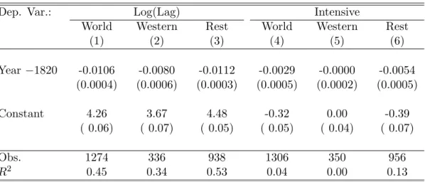
Table 3: Evolution of the Adoption Lag and Intensive Margins

Dep. Var.: Log(Lag) Intensive

World Western Rest World Western Rest

(1) (2) (3) (4) (5) (6)

Year−1820 -0.0106 -0.0080 -0.0112 -0.0029 -0.0000 -0.0054 (0.0004) (0.0006) (0.0003) (0.0005) (0.0002) (0.0005)

Constant 4.26 3.67 4.48 -0.32 0.00 -0.39

( 0.06) ( 0.07) ( 0.05) ( 0.05) ( 0.04) ( 0.07)

Obs. 1274 336 938 1306 350 956

R2 0.45 0.34 0.53 0.04 0.00 0.13

Note: robust standard errors in parentheses. Each observation is re-weighted so that each technology carries equal weight.

4.3 Cross-country evolution of the diffusion process

To analyze the cross-country evolution of the adoption margins in a simple way, we divide the countries in our data set in two groups, as in Maddison (2004): Western countries, and the rest of the world, labeled “Rest of the World”or, simply, non-Western.22

Figure 2a plots, for each technology and country group, the median adoption lag among Western countries and the rest of the world. This figure suggests that adoption lags have declined over time, and that cross-country differences in adoption lags have narrowed. Table 3 formalizes these intuitions by regressing (log) adoption lags on their year of invention (and a constant),

lnDc_τ =ρ+ω·(Invention Yearτ−1820) +εcτ, (31)

where εc_τ denotes an error term. Column (1) reports this regression for the whole sample of countries showing that adoption lags have declined with the invention date. Columns (2) and (3) report the same regression separately for Western and non-Western countries, respectively. We find that the rate of decline in adoption lags is almost a 40% higher in non-Western than in Western countries (1.12% vs. .81%). Hence, there has beenconvergence in the evolution of adoption lags between Western and non-Western countries.

Do we observe a similar pattern for the intensive margin? Figure 2b plots, for each tech-nology and country group the median intensive margin. This figure shows that the gap in the intensive margin between Western countries and the rest of the world is larger for newer than for older technologies. Table 3 studies econometrically this question by regressing the

Figure 2: Evolution of Adoption Margins (a) Convergence of Adoption Lags

(b) Divergence of the Intensive Margin

Note: Bars show median margins of adoption for Western vs. non-Western countries. Technologies: 1. Spindles, 2. Ships, 34. Railway Passengers and Freight, 5. Telegraph, 6. Mail, 7. Steel (Bessemer, Open Hearth), 8. Telephone, 9. Electricity, 101. Cars and Trucks, 12. Tractors, 134. Aviation Passengers and Freight, 15. Electric Arc Furnaces, 16. Fertilizer, 17. Harvester, 18. Synthetic Fiber, 19. Blast Oxygen Furnaces, 20. Kidney Transplant, 21. Liver transplant, 22. Heart Surgery, 23. PCs,

intensive margin on the invention year and a constant,

lnac_τ =ρ+ω·(Invention Yearτ −1820) +εcτ. (32)

Column (6) shows that, for non-Western countries, the intensive margin has declined at an annual rate of .54%.23 Since the intensive margin is measured relative to the mean of West-ern countries, this evidence shows a divergence in the intensive margin of adoption between Western and non-Western countries over the last 200 years.24

4.4 Robustness

We assess the robustness of our estimates and the two cross-country trends in technology diffusion to alternative measurement and estimation approaches.

Curvature The main assumption used in the identification of the adoption margins is that the curvature of the diffusion curve is the same across countries. In our model, this is a consequence of having a common elasticity of substitution between sectoral outputs across countries (i.e., 1/(θ−1)). To explore the empirical validity of this assumption, we re-estimate equation (26) allowingβ_τ3 to differ across countries. Thus, we obtain an estimate ˆβc_τ3 for each country-technology pair. Then, we test whether ˆβc_τ3 in each country is equal to the baseline estimate ˆβ_τ3.We find that in 74% of the cases, we cannot reject the null that the curvature is the same as for the baseline countries at a 5 percent significance level. Table C.3 in the Appendix reports the results of this test for each technology.

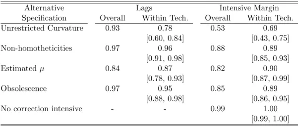
Beyond the statistical validity of the restrictions that our model imposes onβ_τ3,we would like to assess how relevant this assumption is for our main technology adoption estimates. In the first row of Table 4, we report the correlation between the estimates of the diffusion margins in the baseline and in the unrestricted estimations. The first column reports the unconditional correlation of adoption lags across all technologies, which is .93. Then, we estimate this correlation technology by technology. The second column reports the median correlation within technologies, which is .78. We also report the 25th and 75th percentiles of the within technology correlation which are .60 and .84, respectively. We report the same statistics for the intensive margin. The unconditional correlation is .53 and the median correlation within technologies is .69. Based on these statistics, we conclude that the adoption lags and intensive

23

For Western countries, column (5) shows that there is no trend in the intensive margin, as by construction the intensive margin is defined relative to Western countries.

24

One alternative interpretation of Figure2bis that, rather than a continuous decline in the intensive margin in non-Western countries, there was a structural break around 1860. We find that the linear model provides a better statistical fit as measured by the R2. In Section5.3, we examine the implications for income dynamics of modeling the divergence in the intensive margin as a continuous or as a discrete process and show that our results are robust to this modeling choice.

Table 4: Correlation of Baseline Estimates with Alternative Specifications

Alternative Lags Intensive Margin

Specification Overall Within Tech. Overall Within Tech. Unrestricted Curvature 0.93 0.78 0.53 0.69

[0.60, 0.84] [0.43, 0.75]

Non-homotheticities 0.97 0.96 0.88 0.89

[0.91, 0.98] [0.85, 0.93]

Estimatedµ 0.84 0.87 0.82 0.90

[0.78, 0.93] [0.87, 0.99]

Obsolescence 0.97 0.95 0.85 0.89

[0.88, 0.98] [0.86, 0.95]

No correction intensive - - 0.99 1.00

[0.99, 1.00] Note: Overall refers to the correlation of all estimates in the baseline and in the alternative specifi-cation. Within Tech. reports the median correlation of the estimates within technologies. The 25th and 75th percentiles of the correlation within technologies are reported in brackets.

margins that arise under the unrestricted estimation are highly correlated with the baseline estimates.

As important as the robustness of the actual estimates is the robustness of the patterns uncovered for the evolution of the adoption margins. Columns (1) and (2) in Table5report the time-trend coefficient of the (log) adoption lag with respect to the invention date for Western and non-Western countries. Column (3) reports the time-trend coefficient for the intensive margin in non-Western countries (recall that by definition is zero for Western countries). For comparison purposes, we report the baseline estimates in the first row of the table. The new estimates confirm that both the convergence of adoption lags and the divergence in the intensive margin are robust to relaxing the restriction of a common curvature across countries. If anything, the new estimates suggest stronger convergence and divergence patterns than the ones reported in the baseline.

Non-homotheticities We investigate the robustness of our estimates and the dynamics of adoption margins once we allow for non-homotheticities in the demand for technology. Non-homotheticities alter our baseline estimating equation (26) by introducing an income elasticity in the demand for technology, β_{τ y},potentially different from one,

yc_{τ t}=βc_τ1+β_{τ y}y_tc+β_τ2t+β_τ3((µ−1) ln(t−D_τc−τ)−(1−α)(y_tc−lc_t))) +εc_{τ t}. (33) A practical difficulty in estimating (33) is the collinearity of the time-trend and log-income,

Table 5: Time Trend Coefficient Across Alternative Specifications

Dependent Variable: Log(Lag) Intensive

Western Rest World Rest World

(1) (2) (3)

Baseline -0.0080 -0.0112 -0.0054

(0.0006) (0.0003) (0.0005) Unrestricted Curvature -0.0073 -0.0117 -0.0075

(0.0005) (0.0004) (0.0011) Non-homotheticities -0.0082 -0.0118 -0.0044

(0.0006) (0.0005) (0.0006)

Estimated µ -0.0078 -0.0101 -0.0048

(0.0007) (0.0006) (0.0007)

Obsolescence -0.0081 -0.0113 -0.0062

(0.0006) (0.0004) (0.0007)

No correction intensive - - -0.0042

(0.0005) Note: This table reports the coefficientωon the time trend resulting from regressing the (log) adoption lag and the intensive margin onρ+ω(Invention Yearτ−1820) +εcτ for the different

country groupings. Robust standard errors in parentheses. Each technology observation is weighted so that each technology carries equal weight.

common income elasticity for each group.25 Accordingly, we divide the technologies in four groups as a function of their invention data denoted by T ={pre-1850, 1850-1900, 1900-1950, post-1950}. Then, we proceed similarly to the two-step baseline estimation. In the first step, we jointly estimate the income elasticity, β_{T y}, along with β_τ2, and β_τ3 from the diffusion curves of the U.S., UK, and France for each of the four technology groupings. Effectively, this method identifies the income elasticity of technology out of the time series variation in the baseline countries in income and technology. Given that the baseline countries have long time series that for many technologies cover much of its development experience, we consider this to be a reasonable approach.

The estimates of the income elasticity for the technologies invented in the four periods,

β_{T y}, range from 1.58 forT = (pre-1850), to 1.99 for T = (1850-1900).26 The estimates of the slopes of the Engel curves do not vary much across technology groups and they do not have a clear trend.

Once we have obtained the estimates for the income elasticity, we proceed as in the base-line estimation, but instead of imposing an income elasticity of one as our theoretical model suggests, we impose the estimated income elasticity. We estimateβc_τ1andD_τcfor each

country-25_{We have implemented a similar approach grouping the technologies according to the sector rather than the}

invention date, obtaining similar results.

technology pair from the equation

yc_{τ t}=βc_τ1+ ˆβ_{T y}y_tc+ ˆβ_τ2t+ ˆβ_τ3((µ−1) ln(t−D_τc−τ)−(1−α)(y_tc−lc_t))) +εc_{τ t}, (34) where ˆβ_τ2, βˆ_τ3 and ˆβ_{T y} are the values ofβ_τ2, β_τ3 and β_{T y} estimated for the U.S., U.K. and France in the first step.

The estimates of the two margins that we obtain are highly correlated with our baseline estimates. The second line in Table 4 shows that the correlation of adoption lags is .96 and .88 for the intensive margin. Moreover, the patterns of convergence of adoption lags and divergence of the intensive margin remain. The convergence rate (measured as the difference between the coefficients of Western and non-Western countries) is -.44% per year, while in the baseline case it was .31% per year. The divergence rate in the intensive margin is slightly smaller than in the baseline baseline model (−.44%, versus −.54%). However, both trends are statistically and economically robust to allowing for non-homotheticities.

Estimated µ In our baseline estimation, we calibrate the elasticity of substitution between vintages, µ/(µ−1), because it is difficult to separately identify β_τ3 and µ in the baseline diffusion equation (26). However, it is possible to identify them simultaneously in the structural equation that results from substituting expression (14) forzτ in (8) rather than its log-linear

approximation.

In the third row of Table4we compare the adoption margins obtained using this alternative approach with our baseline estimates. Both sets of estimates are similar. Their correlation is .84 for the adoption lags and .82 for the intensive margins. Furthermore, the evolution of the adoption margins across countries quantitatively resembles very much that of our baseline estimates. In fact, we cannot reject the null that the time trends for both adoption lags and the intensive margin are the same as in the baseline estimation.

Obsolescence Some technologies eventually become dominated by others. This is for exam-ple the case of the telegraph which was rendered obsolete by the telephone. The obsolescence of technology may affect the shape of the diffusion curves (especially in the long run) and therefore the estimates of our adoption margins. Since our theory just concerns the diffusion process (and is silent about the phase out process) it does not provide any guide on how ob-solescence impacts our technology measures. As a robustness check, we re-estimate equation (26) over a time sample where obsolescence dynamics are unlikely to be relevant. For each technology, we censor the sample at the point where the leading country starts to experience a decline in the per capita adoption level.27 _{This affects the estimation period in six of the}

twenty-five technologies in our sample. Table 4reports the correlation between the estimates

27

More precisely, we censor all observations that are 90% below the peak level of technology usage for the leading country (after the peak has been attained). This is to allow for some fluctuations in the level of adoption.

of the adoption margins for the censored and uncensored samples. The correlation between the adoption lags is .97, while for the intensive margin it is .85. The evolution of the adoption margins is also robust to controlling for the potential obsolescence of technologies. The rates of decline of the adoption lags for Western and non-Western countries are virtually the same as in the baseline.The divergence in the intensive margin is slightly more pronounced than in our baseline (0.62% vs. 0.54%). Therefore, we conclude that the potential obsolescence of technologies does not affect the trends in adoption patterns we have uncovered.

Measurement of the intensive margin In our baseline estimation, we identify the inten-sive margin by removing from the intercept β_τ1 the productivity gains arising from the timing of adoption. This effect operates through the adoption lag, which we subtract according to (30),

ln ˆac_τ = β

c

τ1−βW esternτ1

β_τ3 +

γ

2(D

c

τ −DW esternτ ).

In our theory, correcting for differences in adoption lags in the intercept has a clear interpre-tation. For the intensive margins to be comparable across countries, they should be computed as if adoption had started at the same time in all countries. This way, any remaining ver-tical differences in the resulting corrected diffusion curves can be attributed to differences in penetration rates of the technology.

However, in the light of the convergence in adoption lags, one might worry that the di-vergence in the intensive margin that we find is a mechanical result inherited from the trends in the estimated adoption lags. Alternatively, one can simply report the intercept without correcting for differences in adoption lags as a less structural benchmark. To address these concerns, we compute an alternative measure of the intensive margin under the assumption that the productivity growth of a technology is zero, γ = 0. Note that, in this case, there is no correction in the intensive margin arising from differences in the timing of adoption. This variation does not affect the estimates of the adoption lags.

The fifth row in Table 4 shows the correlation between these estimates of the intensive margin and our baseline estimates. The overall correlation between these two estimates is .99. The divergence in the intensive margin is also robust to this alternative computation of the intensive margin. In particular, the time trend on the intensive margin for non-Western countries is −.42%, compared to−.54% in our baseline estimate.

5

Income Dynamics

In this section, we evaluate quantitatively the implications of the cross-country patterns of technology diffusion for the evolution of the world income distribution. We focus on three questions: (i) the model’s ability to generate pre-industrial income differences, (ii) the

pro-tractedness of the model’s transitional dynamics, and (iii) the model’s account of the Great Divergence.

5.1 Calibration

To simulate the evolution of productivity growth we use equation (17), which expresses ag-gregate productivity in terms of the sectoral adoption patterns. This requires specifying the evolution of the technology frontier, calibrating four parameters and specifying the evolution of the adoption margins.

We model the evolution of the technology frontier as a one time increase in the growth rate of the frontier. According to Mokyr (1990) and Crafts (1997), an acceleration in the technology frontier growth captures well the Industrial Revolution. We assume that prior to yearT = 1765 (year in which James Watt developed his steam engine), the technology frontier grew at 0.2%.28 This is the growth rate of Western Europe from 1500 to 1800 according to Maddison (2004). After 1765, the frontier growth rate, χ+γ, jumps to (1−α) ·2% per year. This ensures that Modern growth along the balanced growth path is 2%. As previously discussed, we set α=.3. In our baseline simulation, we split evenly the sources of growth in the frontier between γ and χ.29 _{Finally, we calibrate the elasticity of substitution in the final}

good production function, 1/(θ−1), using the average estimates ofβ_τ3,which implies a value of θ= 1.28.

To specify the adoption margins, which also enter equation (17), we assume that they evolve continuously between 1765 and 1983 as described by equations (31) and (32). Prior to 1765 and after 1983, the adoption margins remain constant.30 Constant adoption margins at the end and the beginning of the sample ensure that the economies transition between the two balanced growth paths described by equation (23).

5.2 Cross-country evolution of income growth

We consider the implications of technology dynamics for the evolution of income growth for various country classifications. We begin our analysis with the division between Western and non-Western countries. Then, we divide countries by their income in five quintiles to characterize the evolution of the world income distribution more finely. Finally, we classify

28_{Alternatively, we can set, without any significant change to our findings, the beginning of the Industrial}

Revolution at 1779, year of invention of the first technology in our sample, the mule spindle.

29

From our reading of the literature, it is unclear what fraction of frontier growth comes from increases in productivity due to new technologies (χ) and new vintages (γ). In Section4.4we conduct robustness checks on this division.

30_{We select 1983 as our end date because this is the last invention year in our data (the internet). For the}

adoption lag, and given that it tends towards zero at the end of the sample, similar results would emerge if we allowed for a continuing trend. For the intensive margin, and given our finding of divergence, allowing for a continuing trend would exacerbate the differences between Western and non-Western countries.

countries by their continent and study the implications of the adoption trends observed in each continent for their evolution of income growth.

We start simulating the evolution of output for Western countries and the rest of the world. As discussed in the calibration section, we feed a (common) one time permanent increase in frontier growth and the estimated evolutions for adoption lags and the intensive margin for each group of countries reported in Table 3.

Prior to the adoption of Modern technologies, both groups of countries are in the pre-Modern balanced growth path. Along the pre-industrial balanced growth path, differences in productivity are entirely due to differences in adoption levels of the pre-Modern era. We assume that pre-Modern levels of adoption coincide with the adoption levels that we estimate for the beginning of our sample. Our estimates from Table3imply that the difference between the average adoption lag in the sample of Western countries and the rest of the world is 49 years in 1820. The average gap in the (log) intensive margin is 0.39. Using Maddison’s estimates of pre-industrial growth in Western Europe (0.2%) to calibrate the pre-industrial growth rate of the world technology frontier, equation (23) implies an income gap between Western countries and the rest of the world of 90%.31 This is in line with the results fromMaddison(2004), who reports an income gap of the same magnitude.

After the increase of frontier growth in 1765, countries can start adopting Modern tech-nologies that embody higher productivity. As a result, they increase their productivity growth and transition to the Modern balanced growth path. We report in Figure 3 the evolution of growth rates for the 1765-2000 period.32 Figure 3a shows that the model generates sustained differences in the growth rates of Western and non-Western countries for long periods of time. In the Western economy, output growth starts to accelerate around 1830, and it reaches the steady state growth rate of 2% after 1900. The transitional dynamics implied by the model are very protracted: the half-life of the growth rate is a hundred years. Growth in the non-Western economy does not take off until approximately 1870. After that, it accelerates at a slower pace than the average Western economy. By year 2000, it is still 1.5%. As shown in figure 3b, the resulting gap in growth rates between Western and non-Western economies is considerable. The average annual growth rate is 0.65 percentage points lower in non-Western countries over a period of 180 years. The gap peaks around 1913 at 1%. From then on, the gap declines monotonically until reaching 0.6% by 2000.

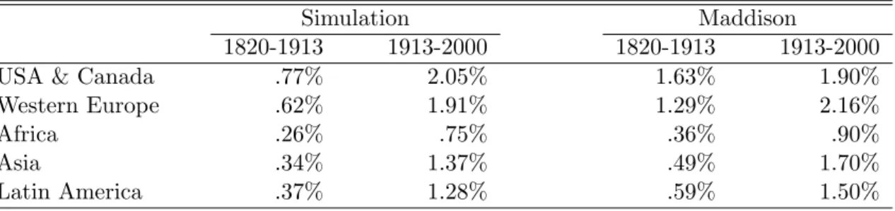
Table6reports the average growth and growth gaps of our simulation and in theMaddison (2004) data. The evolution of productivity growth in both country groups traces quite well

31

That is, exp(.2%·49 +.39/(1−α)) = 1.9.

32_{In the working paper version (Comin and Mestieri,2013), we characterize analytically the transition after}

a permanent increase in the growth rate of the technology frontier and after changes in the adoption margins. We show that the path of the growth rate during the transition is S-shaped. We also provide approximate expressions for the half-life of the system during the transition. We show that the half-life depends on both adoption margins, and that it is an order of magnitude larger than in conventional calibrations of the neoclassical model.

Figure 3: World Income Dynamics, 1820-2000

(a) Output Growth: Western vs. non-Western (b) Difference in Growth Rates

Note: Growth rates of Western countries and the rest of the World obtained imputing the estimated evolution of the intensive and extensive margins using the baseline calibration. Western countries are defined as inMaddison (2004).

the data, though the model slightly underpredicts growth during the nineteenth century. The sustained cross-country difference in growth rates generated by the model accumulate into a 3.2-fold income gap between the Western countries and the rest of the world from 1820 to 2000. Maddison(2004) reports an actual income widening by a factor of 3.9. Hence, differences in the technology adoption patterns account for 82% of the Great Income Divergence between Western and non-Western countries over the last two centuries. When compounding the increase in the gap with initial income differences in 1820, it follows that differences in technology imply an income gap between Western and non-Western countries of 6.2 (1.9·3.2) by 2000. This represents 86% of the 7.2-fold gap reported by Maddison(2004).

The simulation does also well in replicating the time series income evolution of each country group separately. For Western countries, Maddison (2004) reports a 18.5-fold increase in income per capita between 1820 and 2000. Approximately 19% of this increase occurred prior to 1913. In our simulation, we generate a 14-fold increase over the same period, and 16% of this increase is generated prior to 1913. For non-Western countries, Maddison(2004) reports an almost 5-fold increase, with around 37% of the increase being generated prior to 1913. Our simulation generates a 4.3-fold increase in the 1820-2000 period with 32% of this increase occurring in pre-1913. The fact that we underpredict the time series increase in output reflects, in our view, that we are not accounting for the accumulation of factors of production over this time period (e.g., human capital), which also contributed to income growth.

Mechanisms at Work We next decompose the mechanisms at work in our simulation: the acceleration of the technological frontier and the evolution of the two adoption margins. We start by simulating the dynamics of our model after a common acceleration of the technol-ogy frontier for both countries, keeping constant the adoption margins at their initial levels. Figure 5 shows that these initial conditions are an important source of cross-country income divergence. Longer adoption lags in the non-Western country imply a delay of 80 years to

Table 6: Growth rates of GDP per capita Time Period

1820-2000 1820-1913 1913-2000

Simulation Western Countries 1.47% .84% 2.15%

Rest of the World .82% .35% 1.31%

Difference West-Rest .65% .49% .84%

Maddison Western Countries 1.61% 1.21% 1.95%

Rest of the World .86% .63% 1.02%

Difference West-Rest .75% .58% .93%

Notes: Simulation results and median growth rates fromMaddison(2004). We use 1913 instead of 1900 to divide the sample because there are more country observations inMaddison(2004). The growth rates reported from Maddison for the period 1820-1913 for non-Western countries are computed imputing the median per capita income in 1820 for those countries with income data in 1913 but missing observations in 1820. These represent 11 observations out of the total 50. We do the same imputation for computing the growth rate for non-Western countries for 1820-2000. This represents 106 observations out of 145. For the 1913-2000 growth rate of non-Western countries, we impute the median per capita income in 1913 to those countries with income per capita data in 2000 but missing observations in 1913. These represent 67 observations out of the total of 145.

start benefiting from the productivity gains of the Industrial Revolution. As a result, the income gap increases by a factor of 2.3 by year 2000. The transitional dynamics are very protracted. For example, the half-life of the growth rate of Western countries is 141 years. The half-life of output normalized by the long run trend is 114 years, which is an order of magnitude greater than the neoclassical growth model with a conventional calibration, e.g., Barro and Sala-i-Martin (2003).

To assess the role of adoption lags in cross-country growth dynamics, we simulate the evolution of our two economies as in our baseline model, but keeping the intensive margins at pre-industrial levels (i.e., no divergence). Figure 6a presents the results from this simulation. It shows that cross-country differences in adoption lags are an important driver of income divergence during the nineteenth century. By 1900, the income gap between Western and non-Western countries reaches 2.1, as opposed to 2.6 in the full-blown simulation. Thus, the contribution of the divergence in the intensive margin to income divergence during the nineteenth century is rather small. In the twentieth century, the faster reduction in adoption lags in non-Western countries produces a higher growth rate in non-Western countries. Had the intensive margins remained constant at the pre-industrial levels, the relative income between Western and non-Western countries in 2000 would be similar to the level in 1820 and, therefore, there would not have been a Great Divergence.

To analyze the role of the intensive margin, we simulate the evolution of the two economies as in our baseline model, but keeping the adoption lags constant at their pre-industrial levels. Figure 6b presents the dynamics of income growth in each country. In this simulation, the growth acceleration in non-Western countries starts much later than in the baseline (Figure